Real-time gauge theory simulations from stochastic quantization with optimized updating

We investigate simulations for gauge theories on a Minkowskian space-time lattice. We employ stochastic quantization with optimized updating using stochastic reweighting or gauge fixing, respectively. These procedures do not affect the underlying theory but strongly improve the stability properties of the stochastic dynamics, such that simulations on larger real-time lattices can be performed.

1 Introduction

First-principles simulations for gauge field theories such as quantum chromodynamics (QCD) on a Minkowskian space-time lattice represent one of the outstanding aims of current research. Typically, calculations are based on a Euclidean formulation, where the time variable is analytically continued to imaginary values. By this the quantum theory is mapped onto a statistical mechanics problem, which can be simulated by importance sampling techniques. In contrast, for real times standard importance sampling is not possible because of a non-positive definite probability measure.

Simulations in Minkowskian space-time, however, may be obtained using stochastic quantization techniques, which are not based on a probability interpretation [2, 3]. In Refs. [4, 5] this has been recently used to explore the real-time dynamics of an interacting scalar quantum field theory and $SU(2)$ gauge field theory in $3+1$ dimensions. In real-time stochastic quantization the quantum ensemble is constructed by a stochastic process in an additional “Langevin-time” using the reformulation for the Minkowskian path integral [6, 7]: The quantum fields are defined on a physical space-time lattice, and the updating employs a Langevin equation with a complex driving force in an additional, unphysical “time” direction. Though more or less formal proofs of equivalence of the stochastic approach and the path integral formulation have been given for Minkowskian space-time, not much is known about the general convergence properties and its reliability beyond free-field theory or simple models [7, 8]. Most investigations of complex Langevin equations concern simulations in Euclidean space-time with non-real actions [9, 10].

In Ref. [5] real-time stochastic quantization was applied to quantum field theory without further optimization. For $SU(2)$ gauge theory no stable physical solution of the complex Langevin equation could be observed even for small couplings. The physical fixed point was found to be approached at intermediate Langevin-times, however, deviations occurred at later times. The onset time for deviations could be delayed and physical results extracted, if the real-time extent of the lattice was chosen to be sufficiently small on the scale of the inverse temperature. This procedure provided severe restrictions for actual applications of the method. In contrast, for self-interacting scalar field theory stable physical solutions were observed.

In this paper we investigate real-time stochastic quantization for gauge theories employing an optimized updating procedure for the Langevin process. We consider optimized updating using stochastic reweighting or gauge fixing, respectively. These procedures do not affect the underlying theory but strongly improve the stability properties of the stochastic dynamics. For $SU(2)$ gauge theory in $3+1$ dimensions we demonstrate that gauge fixing leads already to stable physical solution for not too small $\beta\sim 1/g^{2}$, where large $\beta$ correspond to going to the continuum limit of the lattice gauge theory. Where applicable, the results are shown to accurately reproduce alternative calculations in Euclidean space-time. In order to gain analytical understanding and to compare to exact results we also investigate $U(1)$ and $SU(2)$ one-plaquette models.

The paper is organized as follows. In Sec. 2 we briefly review real-time stochastic quantization for non-Abelian lattice gauge theory following Ref. [5]. The $U(1)$ one-plaquette model of Sec. 3.1 is used to introduce the concept of stochastic reweighting in Sec. 3.1.3. The simplicity of the model allows us to compare simulation with analytical results and to investigate in some detail the fixed point structure and convergence properties is Secs. 3.1.4 and 3.1.5. In Sec. 3.2 we consider the $SU(2)$ one-plaquette model and introduce some important notions that will be employed for the optimized updating using gauge fixing for the lattice field theory in Sec. 4. We present conclusions in Sec. 5 and an appendix provides some mathematical details.

2 Real-time gauge theory

Gauge theories on a lattice are formulated in terms of the parallel transporter $U_{x,\mu}$ associated with the link from the neighboring lattice point $x+\hat{\mu}$ to the point $x$ in the direction of the lattice axis $\mu=0,1,2,3$. The link variable $U_{x,\mu}=U^{-1}_{x+\hat{\mu},-\mu}\,$ is an element of the gauge group $G$. For $G=SU(N)$ or $U(1)$ one has $U_{x,\mu}^{-1}=U^{\dagger}_{x,\mu}\,$, however, since we will consider a more general group space in the context of stochastic quantization this will not be assumed. Therefore, we keep $U^{-1}_{x,\mu\nu}$ in the definition of the action, which is described in terms of the gauge invariant plaquette variable

$$U_{x,\mu\nu}\equiv U_{x,\mu}U_{x+\hat{\mu},\nu}U^{-1}_{x+\hat{\nu},\mu}U^{-1}_{x,\nu}\,,$$ (1)

where $U_{x,\nu\mu}^{-1}=U_{x,\mu\nu}\,$. The action on a real-time lattice reads

$$S[U] = -\beta_{0}\sum_{x}\sum_{i}\left\{\frac{1}{2{\rm Tr}{\bf 1}}\left({\rm Tr}\,U_{x,0i}+{\rm Tr}\,U_{x,0i}^{-1}\right)-1\right\}$$ (2)

$$+\beta_{s}\sum_{x}\sum_{i,j\atop i<j}\left\{\frac{1}{2{\rm Tr}{\bf 1}}\left({\rm Tr}\,U_{x,ij}+{\rm Tr}\,U_{x,ij}^{-1}\right)-1\right\}\,,$$

with spatial indices $i,j=1,2,3$. Here the relative sign between the time-like and the space-like plaquette terms reflects the Minkowskian metric, and

$$\beta_{0}\equiv\frac{2\gamma{\rm Tr}{\bf 1}}{g_{0}^{2}}\,\,,\quad\beta_{s}\equiv\frac{2{\rm Tr}{\bf 1}}{g_{s}^{2}\gamma}\,,$$ (3)

with the anisotropy parameter $\gamma\equiv a_{s}/a_{t}$ on a lattice of size $(N_{s}a_{s})^{3}\times N_{t}a_{t}$. Because of the anisotropic lattice we have introduced the anisotropic bare couplings $g_{0}$ for the time-like plaquettes and $g_{s}$ for the space-like plaquettes.

Using stochastic quantization the real-time quantum configurations in 3+1 dimensions are constructed by a stochastic process in an additional (5th) Langevin-time [6, 7, 3]. For a discretization with stepsize $\epsilon$ the Langevin-time after $n$ steps is $\vartheta_{n}=n\epsilon$. The discretized Langevin equation for the link variable reads with the notation $U^{\prime}_{x,\mu}\equiv U_{x,\mu}(\vartheta_{n+1})$ and $U_{x,\mu}\equiv U_{x,\mu}(\vartheta_{n})$ [5]

$$U^{\prime}_{x,\mu} = \exp\left\{i\sum_{a}\lambda_{a}\left(\epsilon\,iD_{x\mu a}S[U]+\sqrt{\epsilon}\,\eta_{x\mu a}\right)\right\}U_{x,\mu}\,,$$ (4)

where differentiation in group space is defined by

$$D_{x\mu a}f(U_{x,\mu})=\frac{\partial}{\partial\omega}\,f\left(e^{i\omega\lambda_{a}}U_{x,\mu}\right)|_{\omega=0}$$ (5)

with the generators $\lambda_{a}$ of the Lie algebra and $a=1,\ldots,N^{2}-1$ for $SU(N)$. For the action (2) one has

$$iD_{x\mu a}S[U] = -\frac{1}{2N}\sum_{\nu=0\atop\nu\neq\mu}^{3}\beta_{\mu\nu}{\rm Tr}\left(\lambda_{a}U_{x,\mu}C_{x,\mu\nu}-\bar{C}_{x,\mu\nu}U^{-1}_{x,\mu}\lambda_{a}\right)\,,$$ (6)

where we have defined $\beta_{ij}\equiv\beta_{s}$, $\beta_{0i}\equiv\beta_{i0}\equiv-\beta_{0}$ and

$$C_{x,\mu\nu} = U_{x+\hat{\mu},\nu}U^{-1}_{x+\hat{\nu},\mu}U^{-1}_{x,\nu}+U^{-1}_{x+\hat{\mu}-\hat{\nu},\nu}U^{-1}_{x-\hat{\nu},\mu}U_{x-\hat{\nu},\nu}\,,$$

$$\bar{C}_{x,\mu\nu} = U_{x,\nu}U_{x+\hat{\nu},\mu}U^{-1}_{x+\hat{\mu},\nu}+U^{-1}_{x-\hat{\nu},\nu}U_{x-\hat{\nu},\mu}U_{x+\hat{\mu}-\hat{\nu},\nu}\,.$$ (7)

With $U_{x,\mu}C_{x,\mu\nu}=U_{x,\mu\nu}+U_{x,\mu(-\nu)}$ and $\bar{C}_{x,\mu\nu}U^{-1}_{x,\mu}=U_{x,\mu\nu}^{-1}+U_{x,\mu(-\nu)}^{-1}$ one observes that the sum in Eq. (6) is over all possible plaquettes containing $U_{x,\mu}\,$. Following Ref. [5] the Gaussian noise $\eta_{x\mu a}\equiv\eta_{x\mu a}(\vartheta_{n})$ appearing in (4) is taken to be real and satisfies

$$\langle\eta_{x\mu a}\rangle=0\,,\qquad\langle\eta_{x\mu a}\,\eta_{y\nu b}\rangle=2\,\delta_{\mu\nu}\delta_{xy}\delta_{ab}\,.$$ (8)

Expectation values for observables can be obtained from solving equation (4) for sufficiently large Langevin-time by performing noise averages or, alternatively, from Langevin-time averages [11].

For instance, specifying to $SU(2)$ gauge theory $\lambda_{a}=\sigma_{a}$ ($a=1,2,3$) represent the Pauli matrices, and one can make further simplifications using ${\rm Tr}(U^{-1}\sigma^{a})=-{\rm Tr}(U\sigma^{a})$ for any element $U\in SU(2)$. The latter simplification also holds for $U\in SL(2,{\bf C})$. This is relevant since possible solutions of Eq. (4) may respect this enlarged symmetry group. Taking

$$U_{x,\mu}\equiv e^{iA_{x\mu a}\sigma_{a}/2}$$ (9)

the vector fields $A_{x\mu a}$ need not to be real for $U\in SL(2,{\bf C})$. The complex matrix $A_{x\mu}^{a}\sigma_{a}$ still remains traceless, however, the Hermiticity properties are lost. As a consequence, it is no longer possible to identify $U^{\dagger}$ with $U^{-1}$ as is taken into account in Eq. (2). This corresponds to an extension of the original $SU(2)$ manifold to $SL(2,{\bf C})$ for the Langevin dynamics. Only after taking noise or Langevin-time averages, respectively, the expectation values of the original $SU(2)$ gauge theory are to be recovered. Accordingly, if the Langevin flow converges to a fixed point solution of Eq. (4) it automatically fulfills the infinite hierarchy of Dyson-Schwinger identities of the original theory [5, 12].

3 Optimized updating: simple examples

3.1 One-plaquette model with $U(1)$ symmetry

3.1.1 Direct integration

As a first example we consider the one-plaquette model with $U(1)$ symmetry. For $U=e^{i\varphi}$ the action is given by

$$S_{0}\,=\,\frac{\beta}{2}\left(U+U^{-1}\right)\,=\,\beta\cos\varphi\,$$ (10)

with real coupling parameter $\beta$. The one-plaquette ”partition function” is

$$Z_{0}\,=\,\int_{0}^{2\pi}{\rm d}\varphi\,{\rm e\,}^{iS_{0}}\,=\,2\pi J_{0}(\beta)\,,$$ (11)

where $J_{0}(\beta)$ denotes a Bessel function of the first kind [13], with $J_{0}(1)\simeq 0.765$. The average of an observable $O(\varphi)$ is obtained as

$$\langle O\rangle_{0}\,=\,\frac{1}{Z_{0}}\int_{0}^{2\pi}{\rm d}\varphi\,{\rm e\,}^{iS_{0}}\,O(\varphi)\,.$$ (12)

For real $\beta$ the integrand in Eq. (12) is not positive definite, which mimics certain aspects of more complicated theories in Minkowskian space-time that will be considered below. In contrast to those more realistic theories, the one-plaquette model has the advantage that the elementary integrals can be performed and the results directly compared to those obtained from stochastic methods.

3.1.2 Complex Langevin equation

In principle, adding a Langevin-time dependence $\varphi\to\varphi(\vartheta_{n})$ all observables can be computed from a solution of the discretized Langevin equation

$$\varphi^{\prime} = \varphi+i\epsilon\,\frac{\partial S_{0}(\varphi)}{\partial\varphi}+\sqrt{\epsilon}\,\eta$$ (13)

$$= \varphi-i\epsilon\,\beta\sin\varphi+\sqrt{\epsilon}\,\eta\,,$$

using a notation as in Eq. (4). The real Gaussian noise fulfills

$$\langle\eta\rangle\,=\,0\quad,\qquad\langle\eta\eta\rangle\,=\,2$$ (14)

according to Eq. (8).

In view of the aim to compute plaquette averages, we consider the average of the function $e^{il\varphi}$ with integer $l$. We first compute averages by analytic or direct numerical integration according to Eq. (12), and then compare to the result for the same quantity obtained from a stochastic process using Eq. (13). For $\beta=1$ and $l=1$ one obtains from Eq. (12)

$$\langle e^{i\varphi}\rangle_{0}\,=\,i\,\frac{J_{1}(1)}{J_{0}(1)}\,\simeq\,i\,0.575\,,$$ (15)

which can be compared to the result from the solution of the Langevin equation (13):

$$\langle e^{i\varphi}\rangle_{0}\,\stackrel{{\scriptstyle\rm without\atop optimization}}{{=}}\,-0.009(\pm 0.006)-i\,0.00006(\pm 0.00007)\,.$$ (16)

This result was obtained for $\beta=1$ using a Langevin stepsize $\epsilon=10^{-5}$ from a Langevin-time average over $10^{10}$ steps. The error in brackets gives the statistical fluctuation of the average. One observes that the simulation yields a wrong result that is compatible with zero, in contrast to the non-vanishing imaginary value (15) obtained analytically. A similar failure of the stochastic method can be observed for averages of other functions as well.

3.1.3 Optimized updating by stochastic reweighting

The very same average values as above may be computed with the help of the partition function for a different action $S_{\alpha}\,$,

$$Z_{\alpha} = \int_{0}^{2\pi}{\rm d}\varphi\,{\rm e\,}^{iS_{\alpha}}\,,$$ (17)

from

$$\langle O\rangle_{\alpha} = \frac{1}{Z_{\alpha}}\int_{0}^{2\pi}{\rm d}\varphi\,{\rm e\,}^{iS_{\alpha}}O(\varphi)\,$$ (18)

using standard reweighting techniques. If we define

$$\omega_{\alpha}=e^{i(S_{0}-S_{\alpha})}$$ (19)

then the expectation value (12) can be identically written as

$$\langle O\rangle_{0}\,=\,\frac{\int_{0}^{2\pi}{\rm d}\varphi\,{\rm e\,}^{iS_{\alpha}}\,\omega_{\alpha}\,O(\varphi)}{\int_{0}^{2\pi}{\rm d}\varphi\,{\rm e\,}^{iS_{\alpha}}\omega_{\alpha}}\,=\,\frac{\langle\omega_{\alpha}\,O\,\rangle_{\alpha}}{\langle\omega_{\alpha}\rangle_{\alpha}}\,.$$ (20)

We will consider the family of actions

$$S_{\alpha}\,=\,S_{0}+\alpha\varphi\,=\,\beta\cos\varphi+\alpha\varphi$$ (21)

with integer${}^{\ref{foot:f1}}$ $\alpha$, such that the reweighting function (19) reads

$$\omega_{\alpha}=e^{-i\alpha\varphi}\,.$$ (22)

For the action (21) the discretized Langevin equation is given by

$$\varphi^{\prime} = \varphi-i\epsilon\,\beta\sin\varphi+i\epsilon\,\alpha+\sqrt{\epsilon}\,\eta\,.$$ (23)

As a consequence, for $\alpha\not=0$ the average value in Eq. (20) is computed with the help of a different stochastic process than in Sec. 3.1. For $\beta=1$ and the very same Langevin parameters as above we obtain for $\alpha=1$ the simulation result:

$$\langle e^{i\varphi}\rangle_{0}\,=\,\frac{\langle 1\rangle_{\alpha=1}}{\langle e^{-i\varphi}\rangle_{\alpha=1}}\,=\,-0.001(\pm 0.003)+i\,0.575(\pm 0.0004)\,,$$ (24)

which is close to the exact result given in Eq. (15), in contrast to the failure of the method without reweighting.

$\alpha$	$l$	exact Re	stochastic Re	exact Im	stochastic Im
$0$	$1$	$0$	$-0.00875(\pm 0.006)$	$0.575$	$5.88\!\cdot\!10^{-5}(\pm 7\!\cdot\!10^{-5})$
$0$	$-1$	$0$	$-0.00218(\pm 0.006)$	$0.575$	$8.3\!\cdot\!10^{-5}(\pm 8\!\cdot\!10^{-5})$
$1$	$1$	$0$	$\!-0.000626(\pm 0.0007)\!\!$	$0.261$	$0.261(\pm 0.0005)$
$1$	$-1$	$0$	$-0.00292(\pm 0.007)$	$-1.74$	$-1.74(\pm 0.0005)$
$1$	$2$	$\!-0.0445\!$	$-0.0442(\pm 0.0002)$	$0$	$\!-0.000221(\pm 0.0003)\!$
$1$	$-2$	$1$	$0.998(\pm 0.03)$	$0$	$0.012(\pm 0.03)$
$2$	$1$	$0$	$\!-0.000192(\pm 0.0003)\!\!$	$0.17$	$0.17(\pm 0.0002)$
$2$	$-1$	$0$	$-0.00788(\pm 0.009)$	$-3.83$	$-3.83(\pm 0.0002)$
$2$	$2$	$\!-0.0216\!$	$-0.0216(\pm 6\!\cdot\!10^{-5})$	$0$	$\!-3.5\!\cdot\!10^{-5}(\pm 7\!\cdot\!10^{-5})\!\!$
$2$	$-2$	$-6.66$	$-6.66(\pm 0.03)$	$0$	$0.0338(\pm 0.06)$

Table 1: Averages $\langle e^{il\varphi}\rangle_{\alpha}$ for different values of the reweighting parameter $\alpha$ and fixed $\beta=1$. Listed are results for the real and imaginary part of $\langle e^{il\varphi}\rangle_{\alpha}$ denoted as Re and Im, respectively. Compared are exact results from direct integration with simulation results using a stochastic process. For the exact values three significant digits are given. For the stochastic method the given error in brackets reflects statistical fluctuations.

In Table 1 we list results for averages using various values of $\alpha$ and fixed $\beta=1$. Shown are the results for Re$\langle e^{il\varphi}\rangle_{\alpha}$ and Im$\langle e^{il\varphi}\rangle_{\alpha}$ both from direct integration (”exact”) of Eq. (18) and using a stochastic process (”stochastic”) according to Eq. (23), where we use the same Langevin parameters for the numerics as before. The first two rows correspond to a reweighting parameter $\alpha=0$, i.e. no reweighting, showing the strong disagreement of simulation and exact results in this case. We obtain similarly bad results as long as $\alpha\lesssim\beta$. In contrast, Table 1 shows for $\alpha=1$ accurate values obtained from simulation. We note that in this case the value for $\beta$ agrees with the value chosen for the reweighting parameter $\alpha$, i.e. $\alpha=\beta=1$. For $\alpha=2$ the results are still accurate, which we observe also for several other $\alpha$ and $\beta$ as long as $\alpha\gtrsim\beta$. We typically need to collect substantially more statistics for negative $l$ to keep statistical errors small as compared to the case with positive $l$, which will be addressed in Sec. 3.1.5.

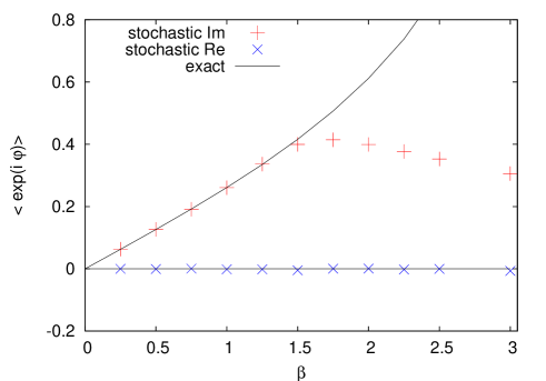
Figure 1: The real and imaginary part of the average $\langle e^{i\varphi}\rangle_{\alpha=1}$ as a function of $\beta$. The lines represent averages obtained from direct integration, while the symbols are measurements using a stochastic process.

The dependence of the accuracy of the simulation outcome on the relative size of $\alpha$ and $\beta$ is further illustrated in Fig. 1, where we consider results for various values of $\beta$ and fixed $\alpha=1$ with $l=1$. Shown are the values for the averages Re$\langle e^{i\varphi}\rangle_{\alpha=1}$ and Im$\langle e^{i\varphi}\rangle_{\alpha=1}$ again from direct integration (lines), which yields

$$\frac{1}{Z_{1}}\int_{0}^{2\pi}{\rm d}\varphi\,e^{i(\beta\cos\varphi+\varphi)}e^{i\varphi} = i\,\frac{J_{2}(\beta)}{J_{1}(\beta)}\,,$$ (25)

as well as using a stochastic process (symbols). One observes that for $\beta\lesssim\alpha$ the simulation method gives accurate results for this quantity, while for somewhat larger $\beta$ they can deviate substantially. In Fig. 2 we show results for $\langle e^{i\varphi}\rangle$ as a function of integer values of $\alpha$ for the case $\beta=\alpha$, which shows very good agreement between stochastic averages and direct integrations.${}^{\ref{foot:f1}}$

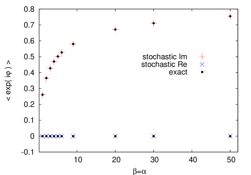
Figure 2: Shown are the real and the imaginary part of the average $\langle e^{i\varphi}\rangle$ as a function of integer $\alpha$ with $\beta=\alpha$.

The above analysis shows that the accuracy of the simulation method depends strongly on the employed stochastic process. It suggests that for a given model there is an optimized stochastic process, which may yield accurate results. The conditions that have to be met in order to obtain quantitative estimates will be further explained in the following.

3.1.4 Fixed point structure

The stationary solutions of the noise averaged Langevin equation (23) are determined by

$$-\beta\langle\sin\varphi\rangle_{\alpha}+\alpha=0\,.$$ (26)

Taking into account that the dynamical variable can become complex with $\varphi=\varphi_{R}+i\varphi_{I}$ this is equivalent to the statement that the equations

$$\langle\cos\varphi_{R}\,\sinh\varphi_{I}\rangle_{\alpha} = 0\,,$$

$$\langle\sin\varphi_{R}\,\cosh\varphi_{I}\rangle_{\alpha} = \frac{\alpha}{\beta}\,,$$ (27)

have to be simultaneously satisfied. Neglecting fluctuations, i.e. disregarding for a moment the noise averages, Eqs. (27) correspond to the classical fixed point condition $\partial S/\partial\varphi\,(\varphi=\varphi^{*})=0$. The first of these equations constrains either $\varphi_{I}=\varphi_{I}^{*}=0$ or $\varphi_{R}=\varphi_{R}^{*}=\pi/2$ or $3\pi/2$ for the real part of the fixed point value. Taking into account the second equation of (27), there are two distinct real solutions for $\beta>|\alpha|$. There are two complex conjugated solutions for $\beta<|\alpha|$ and for $\beta=|\alpha|$ there is a single real solution. We emphasize that these last statements about the possible fixed points just consider the first derivative of the classical action with respect to the dynamical variable, instead of the noise averaged quantity $\langle\partial S/\partial\varphi\rangle$.

The classical approximation becomes exact for $\beta=|\alpha|\to\infty$. In this limit the integral (20) is dominated by the value where the oscillatory integrand shows slowest variation in $\varphi$, i.e. for $\varphi=\varphi^{*}$. As a consequence one obtains

$$\lim\limits_{\beta\to\infty}\frac{\int_{0}^{2\pi}{\rm d}\varphi\,{\rm e\,}^{i\beta(\cos\varphi\pm\varphi)}\,O(\varphi)}{\int_{0}^{2\pi}{\rm d}\varphi\,{\rm e\,}^{i\beta(\cos\varphi\pm\varphi)}}\,=\,O(\varphi^{*})\,,$$ (28)

with $\varphi^{*}=\pi/2$ for the positive sign in the exponent of the integrand, i.e. $\alpha=\beta>0$, and $\varphi^{*}=3\pi/2$ for the negative sign corresponding to $\alpha=-\beta<0$. We will see below that important aspects of the results for finite $\beta$ of Sec. 3.1.3 can be understood already from the classical fixed point condition, i.e. neglecting fluctuations.

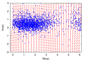
Figure 3: Shown is the real and imaginary part of $\partial S/\partial\varphi$ plotted as a vector with origin at each $\varphi$-value and with normalized length for better visibility. Here we consider $\beta\gtrsim\alpha$, for which the stochastic method fails. For the left graph $1=\beta>\alpha=0$, while the right graph employs $1.5=\beta>\alpha=1$. From the arrows one can infer the two non-attractive, classical fixed points on the real axis. Also shown is the distribution of $\varphi$ as obtained from the full solution of the respective complex Langevin equation. One observes relatively wide distributions with values having positive as well as negative imaginary parts. This has to be compared to Fig. 4 below for the case $\beta\lesssim\alpha$.

For Fig. 3, we have evaluated $\partial S/\partial\varphi$ for the range of values $0\leq\varphi_{R}\leq 2\pi$ and $-\pi\leq\varphi_{I}\leq\pi$ and plotted its real and imaginary part as a vector with origin at each $\varphi$-value. The size of the real and imaginary part of $\partial S/\partial\varphi$ determines the direction and angle of each vector, however, we normalized their length for better visibility. The left figure employs $\alpha=0$, for which one infers from Eqs. (27) two classical fixed points at $\varphi^{*}=0$ and $\varphi^{*}=\pi$. From the arrows it can be seen that these do not correspond to attractive fixed points, where the drift term in the Langevin equation (13) would tend to focus the Langevin flow. Instead they are ”circular” with opposite rotation directions for the two points. Taking into account the $2\pi$-periodicity of the dynamical variable one observes that the fixed points are equidistantly separated along the real axis in this case.

These properties of the classical fixed point determine to a large extend the full Langevin flow, i.e. the behavior of the dynamical variable in the presence of fluctuations due to the noise term $\sim\eta$ in Eq. (23). In order to visualize the distribution of $\varphi$, we make snapshots of the Langevin process with a time-step of $\Delta\vartheta=1$, and plot the values in the complex plane. The resulting distribution for $1=\beta>\alpha=0$, i.e. without reweighting, is given in the left graph of Fig. 3. One observes that the values are rather evenly distributed along the real axis and very loosely centered around it in the complex plane.

For comparison the right graph of Fig. 3 shows the corresponding results for $1.5=\beta>\alpha=1$. One observes the two circular fixed points, which are, however, no longer equidistantly distributed along the real axis. Accordingly, the distribution obtained from the full Langevin dynamics varies considerably along the real axis, with a larger density of points where the classical fixed points are closest to each other. The larger value for $\beta$ compared to the one employed for the left graph leads to a smaller width of the distribution in the complex plane. However, in contrast to the case $\alpha=0$, one observes that the values for the reweighted theory are predominantly localized in the positive-$\varphi_{I}$ half-plane.

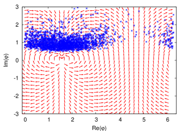
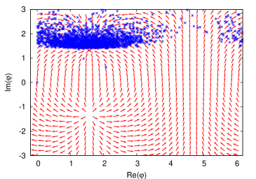
Figure 4: Same as in Fig. 3 but for $\beta=\alpha=1$ (left) and $0.5=\beta<\alpha=1$ (right). For $\beta=\alpha$ one observes the real fixed point with all arrows pointing towards it for positive imaginary part and away from it for negative imaginary part of the dynamical variable. For $\beta<\alpha$ an attractive fixed point in the positive-$\varphi_{I}$ half-plane and a repulsive one in the lower half-plane appears. The comparably narrow distribution for $\varphi$ shows that the Langevin flow spends practically all the time near the attractive side with positive imaginary parts. For the considered cases, where $\beta\lesssim\alpha$, the stochastic method is found to give quantitative results.

The latter tendency continues when $\beta$ is decreased with respect to $|\alpha|$. The left graph of Fig. 4 shows results for $\beta=\alpha=1$, for which only one classical fixed point at a real value appears. This stationary point is neither attractive nor repulsive, with all arrows pointing towards the fixed point for positive imaginary part of $\varphi$ and away from it for negative imaginary part. From the distribution in the left graph of Fig. 4 one observes that the dynamical variable spends most of the Langevin-time near the attractive side of the fixed point. Finally, for $0.5=\beta<\alpha=1$ the two complex fixed points are visible from the right graph of Fig. 4. The one in the positive-$\varphi_{I}$ half-plane is attractive with all arrows pointing towards the fixed point, while the other in the negative-$\varphi_{I}$ half-plane is repulsive. Accordingly, the distribution shown in the right graph of Fig. 4 is practically entirely localized in the positive-$\varphi_{I}$ half-plane.

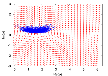
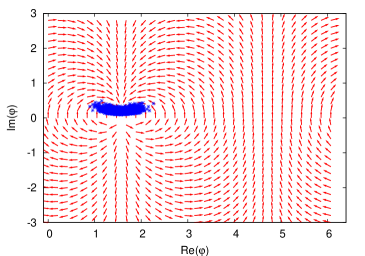
Figure 5: Same as for the left graph of Fig. 4 but for $\beta=\alpha=10$ (left) and $\beta=\alpha=100$ (right).

Fig. 5 shows the same as the left graph of Fig. 4 but with larger $\beta=\alpha=10$ (left) and $\beta=\alpha=100$ (right). As the value for $\beta$ is increased the distribution is more and more centered near the vicinity of the classical fixed point. This reflects the fact that the ($\alpha=\beta$)-reweighted one-plaquette model has a well defined limit $\beta\to\infty$ described by Eq. (28), in which fluctuations are suppressed. This qualitative property of a suppression of fluctuations for large $\beta$ will also be encountered in the discussion for the non-Abelian field theory in Sec. 4.

3.1.5 Convergence

In view of the above findings we consider in the following analytical arguments under which conditions convergence of the stochastic process to accurate results may be expected. For this we associate the stochastic process (23) to a Langevin-time dependent distribution $P_{\alpha}(\varphi;\vartheta_{n})$ for the stochastic variable $\varphi$. Using a notation as in Eq. (23) by writing $P^{\prime}_{\alpha}(\varphi)\equiv P_{\alpha}(\varphi;\vartheta_{n+1})$ and $P_{\alpha}(\varphi)\equiv P_{\alpha}(\varphi;\vartheta_{n})$ its evolution can be obtained from

$$P^{\prime}_{\alpha}(\varphi^{\prime})=\Bigg{\langle}\int{\rm d}\varphi\,P_{\alpha}(\varphi)\,\delta\left(\varphi^{\prime}-\varphi-i\epsilon\,\frac{\partial S_{\alpha}(\varphi)}{\partial\varphi}-\sqrt{\epsilon}\,\eta\right)\Bigg{\rangle},$$ (29)

where the brackets indicate noise average according to Eq. (14). Expanding the $\delta$-functions and keeping only terms up to order $\epsilon$ gives the Fokker-Planck equation

$$\frac{1}{\epsilon}\left(P^{\prime}_{\alpha}-P_{\alpha}\right)(\varphi) = \frac{\partial}{\partial\varphi}\left(\frac{\partial P_{\alpha}}{\partial\varphi}-iP_{\alpha}\,\frac{\partial S_{\alpha}}{\partial\varphi}\right)(\varphi)+{\cal O}(\epsilon)\,.$$ (30)

In the continuum limit $\epsilon\to 0$ we write

$$\frac{\partial P_{\alpha}(\varphi;\vartheta)}{\partial\vartheta} = -H_{FP}(\varphi)P_{\alpha}(\varphi;\vartheta)\,,$$ (31)

with the Fokker-Planck ”Hamiltonian”

$$H_{FP}(\varphi) = -\frac{\partial^{2}}{\partial\varphi^{2}}+i\,\frac{\partial S_{\alpha}(\varphi)}{\partial\varphi}\frac{\partial}{\partial\varphi}+i\,\frac{\partial^{2}S_{\alpha}(\varphi)}{\partial\varphi^{2}}\,.$$ (32)

We first consider the limit of large $\beta=|\alpha|$, where we have seen in Sec. 3.1.4 that the stochastic process converges and is properly governed by the classical fixed point $\partial S/\partial\varphi\,(\varphi=\varphi^{*})=0$. According to Eq. (28) the stationary distribution

$$\lim\limits_{\vartheta\to\infty}P_{\alpha}(\varphi;\vartheta)=P_{\alpha}^{*}(\varphi)$$ (33)

in this case is described by

$$P_{\alpha}^{*}(\varphi)\,\sim\,\lim\limits_{\beta=|\alpha|\to\infty}\frac{e^{iS_{\alpha}(\varphi)}}{Z_{\alpha}}\,\sim\,\delta(\varphi-\varphi^{*})\,.$$ (34)

In order to study the Langevin-time dependence of averages of an observable $O(\varphi)$ in the limit of large $\beta=|\alpha|$, we consider the difference with respect to the stationary solution, i.e.

$$\Delta O(\varphi;\vartheta) \equiv \int{\rm d}\varphi\,O(\varphi)\Delta P_{\alpha}(\varphi;\vartheta)\,,$$ (35)

where $\Delta P_{\alpha}\equiv P_{\alpha}-P_{\alpha}^{*}$ for properly normalized distributions. Since for the classical fixed point the limiting distribution (34) has a compact support away from the boundaries of integration, and assuming analyticity in $\varphi$, we may use partial integration to write:

$$-\hbox to0.0pt{$\displaystyle\int{\rm d}\varphi\,O(\varphi)H_{FP}(\varphi)\Delta P_{\alpha}(\varphi;\vartheta)=$\hss}$$ (36)

$$\int{\rm d}\varphi\,\left(\frac{\partial^{2}O(\varphi)}{\partial\varphi^{2}}+i\,\frac{\partial O(\varphi)}{\partial\varphi}\frac{\partial S_{\alpha}(\varphi)}{\partial\varphi}\right)\Delta P_{\alpha}(\varphi;\vartheta)\,.$$

Since we are interested in plaquette averages, we consider again $O(\varphi)=e^{il\varphi}$ with integer $l$ and $S_{\alpha}(\varphi)$ given by Eq. (21). According to the Fokker-Planck equation (31) the Langevin-time evolution for the observable average (35) is then described by

$$\frac{\partial}{\partial\vartheta}\,\Delta O(\varphi;\vartheta) = -\left(l^{2}+l\alpha\right)\Delta O(\varphi;\vartheta)+l\beta\int{\rm d}\varphi\,\sin(\varphi)O(\varphi)\Delta P_{\alpha}(\varphi;\vartheta)$$ (37)

$$\simeq -\left(l^{2}+l\left[\alpha-\beta\sin(\overline{\varphi})\right]\right)\Delta O(\varphi;\vartheta)\,.$$

For the last approximate relation we used that with Eq. (34) the integrand is peaked near the classical fixed point such that an appropriate constant $\overline{\varphi}$ may be found with $\overline{\varphi}\simeq\varphi^{*}$ in order to simplify the remaining integral and to get a closed equation for $\Delta O(\varphi;\vartheta)$. Eq. (37) has to be evaluated for $\beta=|\alpha|$ but in the notation we keep $\beta$ and $\alpha$ separately for further discussion. The Langevin-time dependence of the observable average is then given by

$$\Delta O(\varphi;\vartheta) \sim e^{-\left(l^{2}+l\left[\alpha-\beta\sin(\overline{\varphi})\right]\right)\,\vartheta}\,.$$ (38)

With

$$\sin(\overline{\varphi})=\sin(\overline{\varphi}_{R})\cosh(\overline{\varphi}_{I})+i\cos(\overline{\varphi}_{R})\sinh(\overline{\varphi}_{I})$$ (39)

one obtains from Eq. (38) a convergent result if

$$l^{2}+l\left[\alpha-\beta\sin(\overline{\varphi}_{R})\cosh(\overline{\varphi}_{I})\right]>0\,.$$ (40)

For $\beta=|\alpha|\to\infty$ we have $\overline{\varphi}=\varphi^{*}$ at sufficiently large $\vartheta$. At the classical fixed point $\partial S/\partial\varphi=\alpha-\sin(\varphi^{*})=0$ which leads to $\lim_{\vartheta\to\infty}\Delta O(\varphi;\vartheta)\sim\lim_{\vartheta\to\infty}e^{-l^{2}\,\vartheta}=0$. Accordingly, the stochastic method is expected to converge well to the stationary solution in this case, which we indeed observe from the full solution of the Langevin equation as described above in Sections 3.1.3 and 3.1.4.

We note that the solution (38) happens to reflect important qualitative properties of the above discussed results also for finite $\beta$ and for $\beta\not=|\alpha|$. The partial integration leading to Eq. (36) is based on analyticity arguments and a compact distribution for the stochastic variable away from the boundaries of integration. The latter is also assumed for the step to the second line of Eq. (37). Of course, in case the dynamics is governed by a classical fixed point, i.e. if the distribution of the dynamical variable is centered around $\overline{\varphi}$ with $\partial S/\partial\varphi(\varphi=\overline{\varphi})\simeq 0$, the condition (40) is automatically fulfilled for any $\beta$ or $\alpha$ because of the fixed point condition (27). However, fluctuations often play an important role and to analytically argue that the Langevin flow not only converges but converges to the correct value is more involved if the dynamics is not governed by a classical fixed point.

The importance of fluctuations can be observed, e.g., from Fig. 2, where for $\beta\lesssim{\cal O}(10)$ substantial deviations from the classical fixed point value occur. If $\partial S/\partial\varphi(\varphi=\overline{\varphi})\not=0$ then the condition (40) can be formally written as

$$\sin(\overline{\varphi}_{R})\cosh(\overline{\varphi}_{I})<\frac{l+\alpha}{\beta}$$ (41)

for $l\not=0$. This suggests that convergent results might be difficult to obtain for $\beta\gg\alpha$, which is indeed in accordance with our findings of Sec. 3.1.3. For instance, in Fig. 1 one observes accurate results for $l=1$ from the stochastic method if $\beta\lesssim\alpha=1$, but a failure of the method for larger $\beta$. This coincides with the fact that for $\beta\lesssim\alpha$ we find a rather compact distribution for $\varphi$ as exemplified in Fig. 4. In this case one observes that the condition (41) is approximately verified if $\overline{\varphi}_{R}$ and $\overline{\varphi}_{I}$ are allowed to take on all $\varphi$-values of significant support. In contrast, for $\beta$ larger than $\alpha$ we find rather wide distributions as exemplified in Fig. 3 and the assumptions leading to (41) may not be justified. In these cases it turns out that the observed distributions are also difficult to reconcile with condition (41). In particular, the case $\alpha=0$ with $\beta=1$ (left graph of Fig. 3) for $l=-1$, which was employed in Sec. 3.1.2 to demonstrate the failure of the stochastic method, is clearly violating that condition. We also verified some further details, e.g., that for $\alpha=1$ and $\alpha=2$ the observable averages with $l=\pm 1$ and $l=\pm 2$ converge faster up to a prescribed statistical error if $l$ is positive, as suggested by condition (41).

3.2 $SU(2)$ one-plaquette model

3.2.1 Direct integration

We consider a theory where the action with real coupling parameter $\beta$,

$$S(U)=\frac{\beta}{2}\,{\rm Tr}\,U\,,$$ (42)

is invariant under the symmetry transformation

$$U\rightarrow W^{-1}UW$$ (43)

with $U,W\in SU(2)$. For the analytical calculations we use a parametrization of $SU(2)$ matrices in terms of an angle $\varphi$ and a unit vector $\vec{n}$:

$$U\left(\varphi,\vec{n}\right)\,=\,e^{i\varphi\vec{n}\cdot\vec{\sigma}/2}\,=\,\left(\cos{\varphi\over 2}\right){\bf 1}+i\left(\sin{\varphi\over 2}\right)\vec{n}\cdot\vec{\sigma}\,,$$ (44)

where $0\leq\varphi<2\pi$ with the three Pauli matrices $\vec{\sigma}$. Using the Haar measure in terms of these variables we obtain averages of an observable $O(U)$ by direct integration from

$$\langle O(U)\rangle = \frac{1}{Z}\int{\rm d}U\,e^{iS(U)}\,O(U)$$ (45)

$$= \frac{1}{Z}\int_{0}^{2\pi}{\rm d}\varphi\int\frac{{\rm d}\Omega(\vec{n})}{4\pi}\,\left(\sin\frac{\varphi}{2}\right)^{2}{\rm e\,}^{i\beta\cos(\varphi/2)}\,O\left(U\left(\varphi,\vec{n}\right)\right)\,,$$

where $\Omega(\vec{n})$ is the uniform measure on the unit sphere and

$$Z = \int_{0}^{2\pi}{\rm d}\varphi\,\left(\sin\frac{\varphi}{2}\right)^{2}{\rm e\,}^{i\beta\cos(\varphi/2)}\,=\,\frac{2\pi}{\beta}\,J_{1}(\beta)\,.$$ (46)

For instance, with ${\rm Tr}\,U/2=\cos(\varphi/2)$ the plaquette average as a function of $\beta$ is

$$\left\langle{1\over 2}{\rm Tr}\,U\right\rangle = i\,\frac{J_{2}(\beta)}{J_{1}(\beta)}\,.$$ (47)

Note that for this particular observable the value of the integral coincides with the one of the plaquette average in Eq. (25) for the ($\alpha=1$)-reweighted $U(1)$ model, and the analytic results are plotted as solid curves in Fig. 1.

3.2.2 Complex Langevin equation

We will compare results obtained from direct integration to estimates from a stochastic process. As described in Sec. 2, this requires an extension of the original $SU(2)$ manifold to $SL(2,{\bf C})$ for the Langevin dynamics. Writing

$$U\,=\,a\,{\bf 1}+i\vec{b}\cdot\vec{\sigma}\,=\,\left(\begin{array}[]{cc}a+ib_{3}&b_{2}+ib_{1}\\ -b_{2}+ib_{1}&a-ib_{3}\end{array}\right)$$ (50)

with ${\rm det}\,U=a^{2}+\vec{b}^{2}=1$ the coefficients $a$ and $\vec{b}$ are complex numbers for $U\in SL(2,{\bf C})$. The Langevin equation follows from Eq. (4). We expand the exponential in that equation to first order in $\epsilon$, which means we must include the square of the noise term, which is proportional to unity. The evolution equation then reads for the one-plaquette model with action (42):

$$U^{\prime} = \left(\tilde{a}\,{\bf 1}+i\sum_{a=1}^{3}\sigma_{a}\left(-\epsilon\,\frac{\beta}{2}\,{\rm Tr}(\sigma_{a}U)+\sqrt{\epsilon}\,\eta_{a}\right)\right)U\,,$$ (51)

with Gaussian noise $\eta_{a}$ corresponding to Eq. (8). In order to stay in group space the constant $\tilde{a}$ in this equation is calculated from $\tilde{a}=\sqrt{1-(-\epsilon\beta{\rm Tr}(\sigma_{a}U)/2+\sqrt{\epsilon}\,\eta_{a})^{2}}$. Alternatively, one can also appropriately normalize that matrix. In contrast to the procedure of Sec. 3.1, Eq. (51) describes the stochastic dynamics directly in terms of group elements $U$. This is closer to what we will do for the $SU(2)$ gauge theory in $3+1$ dimensions in Sec. 4, and is used to introduce some concepts that will be employed for the field theory as well.

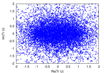
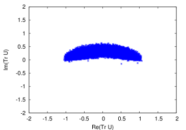
Figure 6: The real and imaginary part of the plaquette variable ${\rm Tr}U$ from snapshots with constant Langevin-time stepping for the $SU(2)$ one-plaquette model with $\beta=1$. The left graph shows the wide distribution of values obtained from the standard Langevin dynamics, while the right graph displays the compact distribution from the (”gauge-fixed”) optimized process (see text for explanation).

Applying the stochastic process to a computation of the plaquette average for $\beta=1$ yields a result consistent with zero:

$$\left\langle\frac{1}{2}\,{\rm Tr}\,U\right\rangle \stackrel{{\scriptstyle\rm without\atop optimization}}{{=}} -0.02(\pm 0.02)-i\,0.01(\pm 0.02)\,,$$ (52)

which disagrees with the non-vanishing exact value $iJ_{2}(1)/J_{1}(1)\simeq i\,0.261$ given by Eq. (47). The situation is analogous to the one described in Sec. 3.1. In particular, the distribution for the stochastic variable obtained from the solution of the Langevin equation (51) exhibits similar qualitative patterns. For instance, the left graph of Fig. 6 shows for $\beta=1$ the distribution of ${\rm Tr}\,U$ in the complex plane. One observes a wide distribution, reminiscent of the left graph shown in Fig. 3 for the $U(1)$ model without optimized updating.

3.2.3 Optimized updating by ”gauge fixing”

An optimized updating scheme for the Langevin dynamics with the aim to calculate accurate results may be achieved in various ways. Motivated by the results of Sec. 3.1, the optimized updating should control the growth of fluctuations for the complex Langevin equation. Since the $SU(2)$ one-plaquette model has a global symmetry described in Eq. (43), which is reminiscent of a local gauge transformation in the corresponding field theory, one may use this symmetry to ”gauge-fix” certain variables in order to constrain the growth of fluctuations. For the complex Langevin equation the plaquette variable $U$ as well as the matrix $W$ in Eq. (43) are elements of $SL(2,{\bf C})$. In the following we will use it in order to diagonalize $U$ after each successive Langevin-time step. For the representation (44) this corresponds to the “gauge-condition” $\vec{n}=(0,0,1)$, or, with the parameterization of Eq. (50) we write after each Langevin updating step $U^{\prime}\,=\,{\rm diag}\left(a+i\sqrt{1-a^{2}},a-i\sqrt{1-a^{2}}\right)$, which corresponds to choosing $\vec{b}=(0,0,\sqrt{1-a^{2}})$.

observable	exact Re	stochastic Re	exact Im	stochastic Im
$\langle{\rm Tr}U/2\rangle$	0	$-0.004(\pm 0.006)$	$0.261$	$0.260(\pm 0.001)$
$\langle({\rm Tr}U/2)^{2}\rangle$	$0.216$	$0.217(\pm 0.003)$	0	$-0.001(\pm 0.002)$

Table 2: Results from the optimized stochastic process, as described in Sec. 3.2.3, are compared to exact values from direct integration for $\beta=1$. For the latter only three significant digits are given. Listed are results for the real and imaginary part of $\langle\rm{Tr}\,U/2\rangle$ and $\langle(\rm{Tr}\,U/2)^{2}\rangle$ denoted as Re and Im, respectively.

Using this procedure we find that, in contrast to the wrong results displayed in Eq. (52) for $\beta=1$, the optimized stochastic process now reproduces correct averages. This is exemplified in Table 2 for two different observables, $\langle{\rm Tr}U/2\rangle$ and $\langle({\rm Tr}U/2)^{2}\rangle$. One can compare the distribution of values obtained from snapshots at equidistant Langevin-time steps with and without optimized updating. The right graph of Fig. 6 shows that the ”gauge-fixing” leads to a compact distribution, in contrast to the one from the unmodified process displayed on the left of that figure. Moreover, for $\langle{\rm Tr}U/2\rangle$ as a function of $\beta$ we obtain a very similar plot than the one shown in Fig. 1 with accurate results for $\beta\lesssim 1$ and wrong results for somewhat larger $\beta$. Of course, according to Eqs. (25) and (47), the expectation values have to coincide in this particular case in the range where correct values are obtained.

We note that the discussion can be performed along very similar lines than what has been done in Sec. 3.1 for the $U(1)$ one-plaquette model. This can be observed from the fact that the above optimized updating procedure can be mapped to a Langevin process with one degree of freedom only, given by

$$\varphi^{\prime}=\varphi-i\epsilon\,\frac{\beta}{2}\sin\frac{\varphi}{2}+\epsilon\,\cot\frac{\varphi}{2}+\sqrt{\epsilon}\,\eta\,$$ (53)

with white noise $\eta$. This Langevin equation follows directly from Eq. (46) by writing the reduced Haar measure as an exponential. The equivalence with the optimized updating is verified explicitly in an expansion of Eq. (51) to order $\epsilon$ in the appendix.

In contrast to the $(\alpha=\beta)$-reweighted one-plaquette model of Sec. 3.1, the $SU(2)$ one-plaquette model has no well-defined limit $\beta\to\infty$, in which fluctuations are suppressed. This can be observed, for instance, from the integral in Eq. (47). For the following discussion it will be an important property that the $SU(2)$ gauge theory has a well-defined limit $\beta\to\infty$, which corresponds to the continuum limit of the lattice theory.

4 $SU(2)$ gauge theory in $3+1$ dimensions

4.1 Stochastic dynamics without optimized updating

Real-time simulations for quantum field theories at non-zero temperature require a complex time-path, where the imaginary-time extent is given by the inverse temperature $\sim 1/T$ and the physical time determines the real-time extent. For scalar and $SU(2)$ gauge theory this has been investigated in Ref. [5] to which we refer for further details. Here we re-consider $SU(2)$ gauge theory. In this case the real-time quantum dynamics in 3+1 dimensions is obtained from a stochastic process in the additional (5th) Langevin-time according to Eq. (4) explained in Sec. 2. The numerical results will be obtained using equal couplings for the time-like and space-like plaquettes in Eq. (3), i.e. $g_{0}^{2}=g_{s}^{2}\equiv g^{2}\sim 1/\beta$ with $N_{s}=4$ and $N_{t}=8$. All values are given in units of appropriate powers of the spatial lattice distance $a_{s}$.

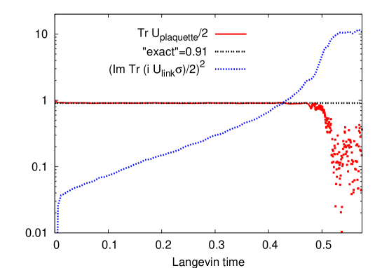
Figure 7: The (red) solid line shows the plaquette variable ${\rm Tr}\,U_{\rm plaquette}/2$ defined in Eq. (54) as a function of Langevin-time using $g=0.5$. We employ a complex contour with non-zero real-time extent at temperature $T=1$ as explained in the text. For comparison, the (black) dashed line gives the corresponding ”exact” result for a Euclidean field theory at the same temperature. Since ${\rm Tr}\,U_{\rm plaquette}/2$ is time-independent, the Langevin-time averages of both results have to agree. The deviation at late Langevin-times is signalled by large values for the squared link variable $\left({\rm Im}\,{\rm Tr}\,(iU_{\rm link}\,\vec{\sigma})/2\right)^{2}$ defined in Eq. (55), which is displayed as a (blue) dotted curve.

In Ref. [5] it was shown that without optimization the Langevin dynamics described by Eq. (4) fails to reproduce correct results in the limit of large Langevin-time. It particular, it was seen that the Langevin flow approaches the correct results at intermediate Langevin-times before it finally starts deviating. This is illustrated in Fig. 7 for the gauge invariant spatial plaquette averaged on the lattice:

$$\frac{1}{2}\,{\rm Tr}\,U_{\rm plaquette}\equiv\frac{1}{6N_{s}^{3}N_{t}}\sum_{x,\,i<j}{\rm Tr}\,U_{x,ij}\,,$$ (54)

where the plaquette variable $U_{x,\mu\nu}$ is defined in Eq. (1). The (red) solid line shows the result as a function of the Langevin-time for a complex (isoceles) triangle contour with real-time extent $\Delta t_{R}=1$ and imginary-time extent $\Delta t_{I}=1$, corresponding to a thermal theory at temperature $T=1$. For comparison, the (black) dashed line gives the ”exact” value for this observable as obtained from stochastic quantization in Euclidean space time, i.e. for a time-contour with no real-time extent. In the latter case one can prove the convergence of the stochastic method [3], and for the employed parameters we find at late Langevin-times ${\rm Tr}\,U_{\rm plaquette}/2=0.91$ giving two significant digits. Of course, this comparison is only possible because we consider the special case of a time-independent observable, whose value has to be the same in Euclidean as well as Minkowskian space-time. From Fig. 7 we see that the result is indeed independent of the employed time-path for not too late Langevin-times. However, finally deviations occur demonstrating the breakdown of the complex Langevin method. In this case the plaquette variable (54) develops larger fluctuations of the imaginary part, whose Langevin-time average is zero, and in Fig. 7 we only show its real part. The onset time for deviations can be delayed by further decreasing the real-time extent of the lattice, which is analyzed in detail in Ref. [5]. In principle this may be used to extract physical results for sufficiently short real times, however, this procedure would provide severe restrictions for actual applications of the method.

A characteristic measure that may be used to monitor this breakdown is given by the quantity

$$\frac{1}{4}\left({\rm Im}\,{\rm Tr}\,(iU_{\rm link}\,\vec{\sigma})\right)^{2}\equiv\frac{1}{4N_{s}^{3}N_{t}}\sum_{x,j}\left({\rm Im}\,{\rm Tr}\,(iU_{x,j}\,\vec{\sigma})\right)^{2}=\frac{1}{N_{s}^{3}N_{t}}\sum_{x,j}\left({\rm Im}\,\vec{b}_{x,j}\right)^{2},$$ (55)

where we used for the last equation the representation corresponding to Eq. (50). This quantity is not gauge invariant and would vanish identically for $U\in SU(2)$. As explained in Sec. 2, for the complex Langevin dynamics $U\in SL(2,{\bf C})$ and, therefore, the quantity $(\ref{eq:ulink})$ can be non-zero and provides a characteristic quantity to measure deviations from $SU(2)$. From the (blue) dotted line of Fig. 7 one observes that the breakdown of the complex Langevin dynamics occurs once this quantity becomes significantly larger than one.

Figure 8: Distributions of the values for the averaged spatial plaquettes ${\rm Tr}\,U_{\rm plaquette}/2$ in the complex plane from snapshots of the Langevin process. The (red) crosses give the distribution for large Langevin-times obtained from the stochastic process without optimization. The (blue) stars give the distribution for large Langevin-times from optimized updating using gauge fixing, which yields correct observable averages. The employed parameters correspond to those used in Figs. 7 and 9.

In order to make contact with the discussions of Secs. 3.1 and 3.2, we display in Fig. 8 the real and imaginary part of the plaquette variable (54) from snapshots with constant Langevin-time stepping. The employed parameters are the same as for Fig. 7. The (red) crosses give the distribution for sufficiently large Langevin-times, i.e. for times when the plaquette variable deviates from the correct results. From Fig. 7 one observes that for the employed parameters this is the case for $\vartheta\gtrsim 0.5$. For these times Fig. 8 exhibits a relatively widespread distribution of values in the complex plane. This is similar to what is observed in Secs. 3.1 and 3.2 for the $U(1)$ and $SU(2)$ one-plaquette models for those cases where the complex Langevin method fails. In contrast, for earlier Langevin-times we find a compact distribution similar to what is displayed as (blue) stars in Fig. 8. Accordingly, for these earlier Langevin-times the values for the plaquette variable (54) agree well with accurate results. The crucial role of a compact distribution for the convergence to accurate results was also observed for the one-plaquette models in Secs. 3.1 and 3.2. In the following, we will show how to stabilize a compact distribution for all Langevin-times using optimized updating by gauge fixing. The (blue) stars in Fig. 8 actually correspond to results obtained from gauge-fixed Langevin dynamics, which will be explained below.

4.2 Optimized updating by gauge fixing

In the previous sections we have observed that the breakdown of the complex Langevin dynamics occurs in the presence of large fluctuations of the complexified dynamical variables. In the spirit of Sec. 3.2, we consider here a reduction of fluctuations by gauge fixing. We employ maximal axial gauge, i.e. on a periodic lattice one can fix by gauge transformations

$$U_{x,\mu}\rightarrow W^{-1}(x)U_{x,\mu}W(x+\hat{\mu})$$ (56)

the link variables to one for the following links:

$$\mu=0,\,\,0\leq x^{0}<N_{t}-1,\,\,0\leq x^{1},x^{2},x^{3}<N_{s}\,,$$

$$\mu=1,\,\,0\leq x^{1}<N_{s}-1,\,\,0\leq x^{2},x^{3}<N_{s},\,\,x^{0}=0\,,$$

$$\mu=2,\,\,0\leq x^{2}<N_{s}-1,\,\,0\leq x^{3}<N_{s},\,\,x^{0}=x^{1}=0\,,$$

$$\mu=3,\,\,0\leq x^{3}<N_{s}-1,\,\,x^{0}=x^{1}=x^{2}=0\,,$$ (57)

where the lattice points are labelled by integers $0\leq x^{1},x^{2},x^{3}<N_{s}$ and $0\leq x^{0}<N_{t}$. The gauge-fixed links are not updated [11] and the rest is updated according to Eq. (4).

Another possibility, which would be the analogue of what was employed for the one-plaquette model in Sec. 3.2, is to update all links but after each Langevin-time step to calculate and apply the field of gauge transformations $W(x)$ in order to fix the link variables according to Eq. (57). One can build up the field of gauge transformations by fixing first $W(0,0,0,0)={\bf 1}$, than get the values $W(0,0,0,z)$ by solving $W^{-1}(x)U_{x,\mu}W(x+\hat{\mu})={\bf 1}$ according to the last line of Eq. (57), than the values $W(0,0,y,z)$ according to the third line, and so on. The latter method turns out to be not as efficient in suppressing fluctuations as the maximal axial gauge.

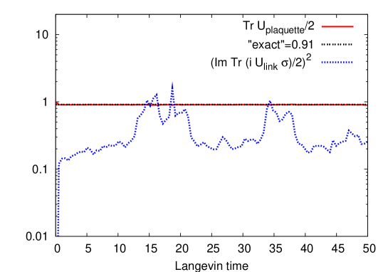
Figure 9: Same as Fig. 7 but with gauge fixing. In contrast to the former, the results from the complex Langevin equation agree well to the ”exact” values even at large Langevin-times. Note that the displayed Langevin-time exceeds the one of Fig. 7 by about a factor of $100$.

In Fig. 9 we show the results corresponding to Fig. 7, however, now obtained from the stochastic dynamics with optimized updating by gauge fixing. One observes that the result from the complex Langevin equation stays close to the ”exact” result and we found no sign of increasing deviations at sufficiently large Langevin-times. Accordingly, also the quantity (55) stays comparably small as displayed in Fig. 9. This reflects the fact that the distribution of the dynamical variable in the complex plane remains relatively compact, which is exemplified in Fig. 8 for the plaquette variable (54).

This is an important advance as compared to the results of Ref. [5], where no stable physical fixed point solution of the Langevin equation could be observed. Gauge fixing turns out to be an efficient way to reduce fluctuations of the complex Langevin dynamics. However, increasing the coupling leads to increased fluctuations and we find that gauge fixing alone is not enough for sufficiently large $g$. Therefore, the combination of gauge fixing and not too large values for the coupling lead to the quantitative results we observe. For the results of Fig. 9 we use $g=0.5$. For the employed parameters with temperature $T=1$, we find that increasing $g$ to values larger than about one leads to deviations from correct results at large Langevin-times similar to the situation displayed in Fig. 7. Decreasing the temperature or using shorter real-time extent improves the situation, as has been found also without gauge fixing in Ref. [5]. We have checked on $N^{3}_{S}=4^{3},...,32^{3}$ lattices that the value of $g$ one has to use for physical results does not depend on the spatial size of the lattice. In principle, this means that even though the small $g$ (and thus larger $\beta$) corresponds to smaller lattice spacings, with a bigger lattice size one could overcome this effect at the expense of computational time. However, in practice this is difficult to achieve for $g<1$ because of limited resources.

The discussion is reminiscent of the one in Sec. 3.1, where it is shown that the ($\alpha=\beta$) reweighted $U(1)$ one-plaquette model is governed by classical dynamics in the limit $\beta\to\infty$. The reduction of fluctuations by increasing $\beta$ in that model is exemplified in Figs. 5 and 4. Qualitatively similar, for the gauge theory one obtains for larger $\beta\sim 1/g^{2}$ more compact distributions than shown in Fig. 8.

5 Conclusions

For the $SU(2)$ gauge theory with action (2) real-time stochastic quantization requires the dynamical variables to become elements of $SL(2,{\bf C})$. The expectation values of the underlying gauge theory are recovered after taking noise or Langevin-time averages, respectively. This change from the compact $SU(2)$ gauge group to the non-compact $SL(2,{\bf C})$ has important consequences for the Langevin dynamics. For the former ${\rm det}U=a^{2}+\vec{b}^{2}=1$ yields finite values for the real $a$ and $\vec{b}$, using the representation of the link variables corresponding to Eq. (50). In contrast, the $SL(2,{\bf C})$ group admits unbounded values for the now complex $a$ and $\vec{b}$. Accordingly, we observe that without optimized updating the complex Langevin equation yields large fluctuations for the dynamical variables at sufficiently late Langevin-times, which finally lead to a breakdown of the method. Apart from the $SU(2)$ gauge theory in $3+1$ dimensions, we observe analogous findings for the $U(1)$ and $SU(2)$ one-plaquette models. The simplicity of the one-plaquette models allow an analytical analysis as presented in Secs. 3.1 and 3.2.

In this paper we showed that large fluctuations of the complexified dynamical variables can be efficiently reduced by employing optimized updating procedures for the Langevin process. Here we investigated optimized updating using stochastic reweighting or gauge fixing, respectively. These procedures do not affect the underlying theory but can stabilize the physical fixed point of the Langevin equation. The success of stochastic reweighting was found to be linked to the appearance of attractive fixed points of the Langevin flow, while the gauge fixing simply constrains the dynamical variables. For the gauge theory we demonstrated that gauge fixing leads to an efficient reduction of fluctuations for not too small $\beta\sim 1/g^{2}$: We employed maximal axial gauge and calculated plaquette averages on a lattice with non-zero real-time extent. Where applicable, the results were shown to accurately reproduce alternative calculations in Euclidean space-time. This is an important advance as compared to the results of Ref. [5], where no stable physical fixed point solution of the Langevin equation could be observed for the non-Abelian gauge theory even for small couplings.

For the reweighted $U(1)$ and the ”gauge-fixed” $SU(2)$ one-plaquette models, we obtained accurate results also for small $\beta$. The fact that real-time stochastic quantization is simpler to apply to non-gauge theories is in accordance with earlier findings for scalar field theories in Ref. [5]. Since large $\beta$ describe the continuum limit of the lattice gauge theory, with the present results at hand one has in principle a procedure to do simulations in non-Abelian gauge theory. However, without further improvements, it is difficult to achieve $g\lesssim 1$ because of limited computational resources. Also further tests using different time contours along the lines of Ref. [5] are necessary before pressing questions of calculations of transport properties and nonequilibrium gauge theory dynamics are to be addressed.

Acknowledgements: We are indebted to Ion-Olimpiu Stamatescu for collaboration in an early stage of a common work on reweighting techniques for one-plaquette models and proposing a modified Langevin equation (23). We also thank Szabolcs Borsányi for helpful discussions and fruitful collaboration on related work. This work was supported in part by the BMBF grant 06DA267, and by the DFG under contract SFB634.

6 Appendix

In this appendix we show that the optimized updating procedure employed for the $SU(2)$ one-plaquette model in Sec. 3.2.3 can be mapped to a Langevin process with one degree of freedom only, described by Eq. (53).

Using the parameterization of Eq. (50) we write $U=a+i\vec{b}\vec{\sigma}$. The ”gauge fixing” condition employed in Sec. 3.2.3 then reads $\vec{b}=(0,0,\sqrt{1-a^{2}})$. We denote in Eq. (51) the Langevin-time-stepping matrix as $\Theta=\tilde{a}+i\vec{d}\vec{\sigma}$. Because $U$ is rotated to the fixed gauge after the last Langevin-time step we have $b_{1}=b_{2}=0$, ${\rm Tr}(\sigma_{1}U)={\rm Tr}(\sigma_{2}U)=0$ and, accordingly,

$$d_{1}=\eta_{1}\sqrt{\epsilon},\ \ \ \ d_{2}=\eta_{2}\sqrt{\epsilon},\ \ \ \ d_{3}=-\epsilon{\beta\over 2}{\rm Tr}(\sigma_{3}U)+\eta_{3}\sqrt{\epsilon}\,.$$ (58)

Multiplying $\Theta$ and $U$, one obtains $U^{\prime}=a^{\prime}+i\vec{b}^{\prime}\vec{\sigma}$ using $b_{1}=b_{2}=0$ and $(\vec{v}\vec{\sigma})(\vec{w}\vec{\sigma})=\vec{v}\vec{w}+i\vec{\sigma}(\vec{v}\times\vec{w})$ :

$$a^{\prime}+i\vec{b}^{\prime}\vec{\sigma}=a\tilde{a}-\vec{b}\vec{d}+i\sigma_{1}(ad_{1}-d_{2}b_{3})+i\sigma_{2}(ad_{2}+d_{1}b_{3})+i\sigma_{3}(\tilde{a}b_{3}+ad_{3})\,.$$ (59)

Again rotating to the fixed gauge one obtains $U^{\prime\prime}=a^{\prime\prime}+i\vec{b}^{\prime\prime}\vec{\sigma}$ with

$$a^{\prime\prime}=a^{\prime},\ \ \ \ b_{1}^{\prime\prime}=b_{2}^{\prime\prime}=0,\ \ \ \ b_{3}^{\prime\prime}=\sqrt{b_{1}^{\prime 2}+b_{2}^{\prime 2}+b_{3}^{\prime 2}}\,.$$ (60)

Expanding $b_{3}^{\prime\prime}$ to order $\epsilon$ according to Eq. (58) leads to

$$b_{3}^{\prime\prime}=(1-{d_{3}^{2}\over 2})b_{3}+a\left(d_{3}+{d_{1}^{2}+d_{2}^{2}\over 2}{a\over b_{3}}\right)\,.$$ (61)

One can write $d_{1}^{2}+d_{2}^{2}=4\epsilon+\epsilon\rho$, where $\rho$ is a noise term with zero mean. Since it is multiplied with $\epsilon$, in the continuum limit one can neglect this term. Using the notation $b_{3}^{\prime\prime}=\sin(\varphi^{\prime\prime}/2)$ and similarly $b_{3}=\sin(\varphi/2)$, and $\Delta\varphi=d_{3}+2\epsilon{a\over b_{3}}$, and noticing that to order $\epsilon$ one has $\cos\Delta\varphi=(1-{d_{3}^{2}\over 2})$ yields

$$\sin{\varphi^{\prime\prime}\over 2}=\cos(\Delta\varphi)\sin{\varphi\over 2}+\cos{\varphi\over 2}\sin(\Delta\varphi)\,.$$ (62)

Since this describes angle addition, we get:

$${\varphi^{\prime\prime}\over 2}-{\varphi\over 2}=d_{3}+2\epsilon{a\over b_{3}}=-i\epsilon\beta\sin{\varphi\over 2}+2\epsilon\cot{\varphi\over 2}+\eta_{3}\sqrt{\epsilon}\,,$$ (63)

which is the discretised Langevin equation (53) as obtained from the “reduced” action $S=2\ln\sin{\varphi/2}+i\beta\cos{\varphi/2}$, with Langevin-time step $4\epsilon$.

References

- [1]
- [2] G. Parisi and Y.-S. Wu , Sci. Sin., Ser. A, Math. Phys. Astron. Tech. Sci. 24 (1981) 483.
- [3] P. H. Damgaard and H. Hüffel, Phys. Rept. 152 (1987) 227.
- [4] J. Berges and I. O. Stamatescu, Phys. Rev. Lett. 95 (2005) 202003 [arXiv:hep-lat/0508030].
- [5] J. Berges, S. Borsanyi, D. Sexty and I. O. Stamatescu, Phys. Rev. D 75 (2007) 045007 [arXiv:hep-lat/0609058].
- [6] J. R. Klauder, in Recent developments in High Energy Physics, edited by H. Mitter and C. B. Lang (Springer, New York, 1983); Phys. Rev. A 29 (1984) 2036. G. Parisi, Phys. Lett. B 131 (1983) 393.
- [7] H. Hüffel and H. Rumpf, Phys. Lett. B 148 (1984) 104. E. Gozzi, Phys. Lett. B 150 (1985) 119. D. J. E. Callaway, F. Cooper, J. R. Klauder and H. Rose, Nucl. Phys. B 262 (1985) 19. H. Nakazato and Y. Yamanaka, Phys. Rev. D 34 (1986) 492. H. Hüffel and P. V. Landshoff, Nucl. Phys. B 260 (1985) 545. K. Okano, L. Schulke and B. Zheng, Prog. Theor. Phys. Suppl. 111 (1993) 313.
- [8] J. Klauder and W. Petersen, J. Stat. Phys. 39 (1985) 53. J. Ambjorn and S. K. Yang, Phys. Lett. B 165 (1985) 140. T. Matsui and A. Nakamura, Phys. Lett. B 194 (1987) 262. H. Okamoto, K. Okano, L. Schulke and S. Tanaka, Nucl. Phys. B 324 (1989) 684. K. Okano, L. Schulke and B. Zheng, Phys. Lett. B 258 (1991) 421. L. L. Salcedo, Phys. Lett. B 305 (1993) 125. K. Fujimura, K. Okano, L. Schulke, K. Yamagishi and B. Zheng, Nucl. Phys. B 424 (1994) 675 [arXiv:hep-th/9311174]. H. Gausterer, J. Phys. A 27 (1994) 1325 [arXiv:hep-lat/9312003].
- [9] F. Karsch and H. W. Wyld, Phys. Rev. Lett. 55 (1985) 2242. J. Flower, S. W. Otto and S. Callahan, Phys. Rev. D 34 (1986) 598. H. Gausterer and J. R. Klauder, Phys. Rev. D 33 (1986) 3678. E. M. Ilgenfritz, Phys. Lett. B 181 (1986) 327. J. Ambjorn and S. K. Yang, Nucl. Phys. B 275 (1986) 18. N. Bilic, H. Gausterer and S. Sanielevici, Phys. Lett. B 198 (1987) 235; Phys. Rev. D 37 (1988) 3684. C. W. Bernard and V. M. Savage, Phys. Rev. D 64 (2001) 085010 [arXiv:hep-lat/0106009].
- [10] J. Ambjorn, M. Flensburg and C. Peterson, Nucl. Phys. B 275 (1986) 375; Phys. Lett. B 159 (1985) 335.
- [11] See e.g. I. Montvay and G. Münster, Quantum Fields on a Lattice (Cambridge University Press, Cambridge, UK, 1997).
- [12] S. Xue, Phys. Lett. B 180 (1986) 275.
- [13] I. S. Gradshteyn and I. M. Ryzhik, Table of Integrals, Series, and Products (Academic Press, 5th ed., 1994).