Long term dynamics of the splitting of a doubly quantized vortex in a two-dimensional condensate

Abstract

We study the nonlinear dynamics of the splitting of a doubly quantized vortex in a trapped condensate. The dynamics is studied in detail by solving the Gross-Pitaevskii equation. The main dynamical features are explained in terms of a nonlinear three-level system. We find an analytical solution for the characteristics of the dynamics. It is concluded that the time scale for the splitting is mainly determined by the instability of the linearized system, and nonlinear effects contribute logarithmically.

I Introduction

Quantization of fluid circulation is one of the most pictorial macroscopic manifestations of quantum mechanics. Lattices of singly quantized vortices have been imaged in superconductors in magnetic fields essmann , liquid helium vinen , and more recently in trapped Bose-Einstein condensates madison2000 ; ketterle2001 . Vortices with higher quantum numbers than unity are energetically unstable in many common situations, including an infinite, homogeneous s-wave superfluid, and the experimentally relevant case of a condensate contained in a parabolic potential Pethick2001 ; butts1999 ; lundh2002 . In addition, in the latter case, multiply quantized vortices are found to be dynamically unstable in large areas of parameter space pu1999 ; jackson2005 ; mottonen2003 . It was predicted that a doubly quantized vortex is unstable towards splitting into two vortices with unit quantum number, in accordance with the quantization of fluid circulation.

These predictions were put to an experimental test in 2004, when a doubly quantized vortex, i.e., a vortex with quantum number 2, was imposed on a stationary condensate and the subsequent splitting was monitored shin2004 . This experiment has been analyzed quantitatively in Refs. mottonen2006 ; mateo2006 using the time-dependent Gross-Pitaevskii equation Pethick2001 , and in Refs. Lundh06 ; huhtamaki2006 by means of Bogoliubov theory. However, there remains to marry together these two approaches. In particular, Bogoliubov analysis gives information only about the linear (i. e., short-time) behavior of the unstable system, while solving the full Gross-Pitaevskii equation gives more detail than is necessary in order to understand the important features of the dynamics.

Dynamics of vortices is a subject with a long history. It is well known that in a incompressible fluid the vortices move with the background fluid velocity kelvin . This is not so in a compressible fluid where the background density changes Nilsen06 . In general, vortex motion in a compressible fluid is complicated and cannot be separated from the dynamics of the system. The splitting of a doubly quantized vortex offers an opportunity to study the vortex dynamics in an extreme regime where the background velocity changes rapidly on the scale of the size of a vortex core. The splitting dynamics therefore offers insight into compressible fluid dynamics. In the study of the linear stability of doubly quantized vortices Lundh06 , it was shown that the stability depends critically on the energy of the surface modes, and thus on global properties not associated with the vortex. The focus of this paper will be on the dynamics after the initial exponential growth of the vortex distance. Even though the experiment of Ref. shin2004 was performed in an elongated three-dimensional geometry, this study is concerned with a two-dimensional system, in order to clearly bring out the structure of the problem.

In this paper, we perform a systematic investigation of the long time behavior of the splitting of two vortices. The paper is organized as follows. In Sec. II we discuss the equations governing the system. In Sec. III we describe the numerical solution of the equations of motion. Section IV is devoted to a calculation of the nonlinear dynamics. The main features of the dynamics are captured in terms of a model that is solved analytically in Sec. V. Finally, in Sec. VI we summarize and conclude. Specifics of the analytical solution are given in the three appendices.

II Splitting of a doubly quantized vortex

The system we study is a Bose-Einstein condensate of particles of mass $m$ that is trapped in a cylindrically symmetric potential. At zero temperature in the dilute limit the gas is described by a condensate wavefunction $\Psi({\mathbf{r}},t)$ that obeys the Gross-Pitaevskii (GP) equation

$$i\hbar\frac{\partial\Psi}{\partial t}=H_{0}\Psi+U_{0}|\Psi|^{2}\Psi,$$ (1)

where

$$H_{0}=-\frac{\hbar^{2}}{2m}\nabla^{2}+V({\bf r}),$$ (2)

and the trapping potential is assumed to be of the form

$$V({{\bf r}})=\frac{m\omega^{2}}{2}(r^{2}+\lambda^{2}z^{2}).$$ (3)

The inter-particle interactions are parametrized by an $s$-wave scattering length $a$, so that $U_{0}=4\pi\hbar^{2}a/m$. We immediately pass to trap units, where the unit of length is the oscillator length $a_{\rm osc}=(\hbar/m\omega)^{1/2}$ and the unit of time is $\omega^{-1}$ Pethick2001 . We assume the system to be two-dimensional (2D), which corresponds to the limit of a very tight trapping potential in the axial direction. The wavefunction in that direction is thus assumed to be in the ground state; on integrating out the $z$ dependence one obtains the effective 2D interaction parameter

$$C=\frac{Na}{a_{\rm osc}}\int|\phi_{0}(z)|^{4}{\rm d}z=\frac{Na\sqrt{\lambda}}{a_{\rm osc}\sqrt{2\pi}},$$ (4)

where $\phi_{0}$ is the ground-state single-particle wave function in a one-dimensional harmonic potential. The resulting equation of motion for the condensate is

$$i\frac{\partial\Psi}{\partial t}=\left[-\frac{1}{2}\nabla^{2}+\frac{1}{2}r^{2}+C|\Psi|^{2}\right]\Psi.$$ (5)

As a starting point for the study of the dynamics it is useful to repeat the linear stability analysis pu1999 ; Lundh06 . The GP equation is expanded about a stationary solution $\Psi({\mathbf{r}},t)=\Psi_{0}({\mathbf{r}})\exp(-i\mu t)$ (which in the present case will be the doubly quantized vortex solution), where $\mu$ is the chemical potential of the system. The ansatz for the expansion is taken to be

$$\Psi({\bf r},t)=\left[\Psi_{0}({\bf r})+\sum_{n}\left(u_{n}({\bf r})e^{-i\omega_{n}t}+v_{n}({\bf r})^{*}e^{i\omega_{n}t}\right)\right]e^{-i\mu t},$$ (6)

where $u_{n}$ and $v_{n}$ are the quasiparticle amplitudes and $\omega_{n}$ the quasiparticle energies calculated from the Bogoliubov equations Pethick2001 . The small-amplitude excitations of the condensate are described by the eigenvectors and eigenvalues of the Bogoliubov equations,

$$B\left(\begin{array}[]{l}u_{n}({\bf r})\\ v_{n}({\bf r})\end{array}\right)=\omega_{n}\left(\begin{array}[]{l}u_{n}({\bf r})\\ v_{n}({\bf r})\end{array}\right),$$ (7)

where the linear operator $B$ is defined by

$$B=\left(\begin{array}[]{cc}H_{0}-\mu+2C|\Psi|^{2}&C\Psi^{2}\\ -C(\Psi^{*})^{2}&-\left(H_{0}-\mu+2C|\Psi|^{2}\right)\end{array}\right).$$ (10)

If $B$ has a complex eigenvalue, the system is dynamically unstable and the corresponding mode will grow exponentially. It is known that there exist intervals of the coupling constant $C$ where the Bogoliubov equations possess a pair of complex eigenvalues. This behavior was thoroughly studied by the present authors in a previous paper Lundh06 (cf. pu1999 ). Figure 1 shows the eigenvalue behavior as a function of $C$ for the 2D case.

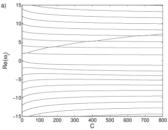
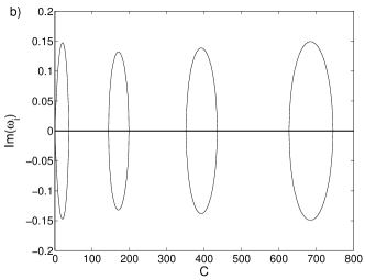
Figure 1: Energy levels in two dimensions for a condensate with an $m=2$ vortex. The left panel shows the real parts and right panel the imaginary parts. All imaginary parts except at most one are zero at any point in this phase space.

An instability occurs when the energies of two Bogoliubov modes collide. In the present case the mode confined to the interior of the vortex, referred to as the core mode, mixes with surface modes of quadrupole symmetry. The core mode is seen in Fig. 1(a) as the line with positive slope that repeatedly merges with other lines representing the energies of quadrupole surface modes; each such collision creates an instability, so that successively higher instability regions correspond to increasing radial quantum number of the quadrupole mode.

The Bogoliubov equations describe only the linear, i. e., small-amplitude, evolution of the condensate. In order to capture the full, nonlinear time development, in general one has to perform a numerical time integration of the time-dependent GP equation (1). However, the purpose of the present paper is to study to what extent a simplified approach, based on the solutions to the Bogoliubov equations, will suffice, and therefore we will in subsequent sections compare the full numerical results to the simplified model. To study the splitting dynamics of a doubly quantized vortex one needs to choose a perturbed doubly quantized vortex as initial condition. The doubly quantized vortex state is a stationary, rotationally symmetric solution of the GP equation (5) of the form

$$\Psi_{2}(r,\theta)=f_{2}(r)e^{i2\theta},$$ (11)

where the real amplitude $f_{2}(r)$ obeys the equation

$$\left[-\frac{1}{2}\left(\frac{1}{r}\frac{\partial}{\partial r}r\frac{\partial}{\partial r}+\frac{2^{2}}{r^{2}}\right)+V(r)+C|f_{2}(r)|^{2}\right]f_{2}(r)=\mu f_{2}(r).$$ (12)

As the initial condition for dynamical simulations one needs to add a perturbation to the doubly quantized vortex state. For definiteness, we have chosen to use the ground-state harmonic oscillator wave function as a perturbation, but as long as the perturbation is small, its exact form does not matter for the long-time evolution, after it is exponentially inflated.

III Numerical method

The GP equation (5) is solved using a Hermite mesh in both spatial directions, and the time evolution is done using a Strang splitting that makes use of the tensor product structure of the linear problem McPeake2002 . For a sufficiently large grid, in our case $100\times 100$ points, we get conservation of angular momentum to one part in $10^{6}$. This symplectic method is nearly optimal for the problem at hand, which was crucial in order to be able to scan the parameter range and to analyze the subtle nonlinear dynamics in detail.

The Bogoliubov equation is solved separately. Due to the cylindrical symmetry, it is reduced to a 1D eigenvalue problem, whose solution was described in Ref. Lundh06 .

One of the most important quantities to be discussed in the following is the distance between two vortices in the numerical time evolution. To measure this distance, we first identify the spatial points ${\bf r}$ which fulfill the criteria $|{\bf r}|<4$ and $|\Psi({\bf r})|<0.15{\rm Max}(\Psi)$; these are the points of low density in the interior of the system. Using these points we do a least-square fit to the form

$$\widetilde{\Psi}(z)=A(z+z_{0})(z-z_{0})e^{-|z|^{2}/2},$$ (13)

where $z$ is short for $z=x+iy$. The fit is done with respect to the two constants $A$ and $z_{0}$. This fitting function describes two vortices placed symmetrically about the origin and is found to be an accurate approximation for the wavefunction at all times, in accordance with the expectation that the instability of a doubly quantized vortex results in the vortex splitting into two. The fit for the parameter $z_{0}$ gives the positions of the two vortices as $z_{0}$ and $-z_{0}$, and the vortex distance is $d=2|z_{0}|$. A good fit is very difficult to achieve for small separations, since the least-square method minimization problem is then very shallow and small numerical errors in the wavefunction $\Psi$ give significant contributions. A more reliable method to find the qualitative time evolution is to notice that in the weakly interacting limit, the squared length $|z_{0}|^{2}$ is approximately proportional to the population of the lowest harmonic-oscillator eigenstate (see Lundh06 , Eq. (23)). Therefore we project the wave function onto the eigenstates of the harmonic-oscillator potential,

$$a_{n,m}(t)=\int\Psi(x,y,t)\phi_{n,m}(x,y)dxdy,$$ (14)

where $\phi_{n,m}$ is the eigenstate of the harmonic-oscillator potential with energy $\omega_{n,m}=2n+|m|+1$,

$$\phi_{n,m}(r,\theta)=\sqrt{\frac{n!}{\pi(n+m)!}}L_{nm}(r^{2})\left(re^{i\theta}\right)^{m}e^{-r^{2}/2},$$ (15)

and

$$L_{n\alpha}(x)=\sum_{j=0}^{n}(-1)^{j}\binom{n+\alpha}{n-j}\frac{1}{j!}x^{j}$$ (16)

is a generalized Laguerre polynomial. The population of an excited state is defined as

$$P_{0,m}(t)=|a_{0,m}(t)|^{2}.$$ (17)

The integral in Eq. (14) is calculated using the Gauss-Hermite quadrature rule associated with the Hermite mesh, which is exact in the limit of low energies. As we shall se, we find the amplitudes $P_{n,m}$ useful for understanding the dynamics of the problem.

IV Time development of vortex splitting

As known from previous studies pu1999 ; Lundh06 , the dynamics of a perturbed doubly quantized vortex falls into one of two categories depending on the value of the coupling strength $C$. In some intervals the doubly quantized vortex is stable and in others it is unstable, as investigated in detail in Ref. Lundh06 . The real and imaginary parts of the Bogoliubov eigenvalues are presented in Fig. 1. The regions where the vortex is linearly stable are not interesting from a dynamical perspective when small perturbations are considered. The condensate will just perform small periodic oscillations following the initial perturbation. Thus the domains of interest are the unstable regions. It turns out that these can roughly be divided into two: the first unstable region, and all the subsequent ones.

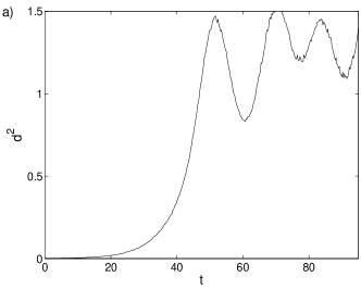
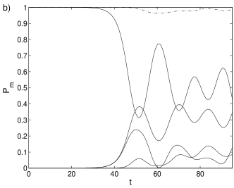
Figure 2: (a) Time development of the vortex distance $d$, and (b) time development of the populations $P_{m0}(t)$ of the harmonic-oscillator eigenstates, for a two-dimensional condensate with coupling parameter $C=20$. In (b), the curves represent from the bottom up, $m=6$, $m=4$, $m=0$, $m=2$, and the sum of all four. The initial state was perturbed by means of a seeding of the harmonic oscillator ground state with an amplitude $P_{00}=0.001$.

We first consider the first unstable region, $C\in[0,37]$. An example of the dynamics is given in Fig. 2. The depletion of the condensate, i. e. the $m=2$ state, is very strong. It is seen that the sum of the populations in the $m=0$, 2, and 4 states is less than 1 after some time, which means that there is a non-negligible population in states with $m>4$. (Although the negligible population of states with odd $m$ is here a consequence of the chosen initial conditions, we have checked that for more general initial conditions it is enforced by the dynamics, since only modes with even $m$ become dynamically unstable.) The population in states with $m>4$ is seeded by the large population in the $m=4$ state, as will be clear below. Another feature which is worth noticing is that the vortex distance is highly correlated with the $m=0$ population, as anticipated in Sec. IV. We take advantage of this near proportionality to find the time dependence of the vortex distance when the fitting method to find the vortex position described in Sec. IV fails.

The time evolution proceeds in two stages. From the start the population of the $m=0$ state (which is the perturbation inserted by hand) and the $m=4$ state grow exponentially while the condensate, the $m=2$ state, is accordingly depleted. After the population of the $m=0$ and $m=4$ states has become non-negligible, the populations of the two amplified states becomes asymmetric, due to population of higher-angular momentum states. The vortex distance and the population will start oscillating around finite values. Later we will see that the asymmetry and the population of higher-angular momentum eigenstates are crucial for the vortex distance to not oscillate back to zero. It is important to note that the asymmetry between the $m=0$ and $m=4$ populations is not caused by the initial population chosen here, but is enforced by the dynamics.

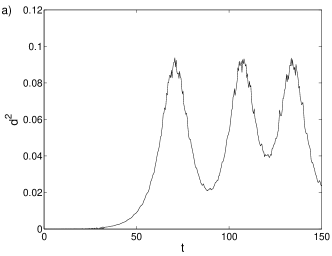
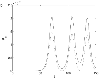
Figure 3: (a) Square of the vortex distance $d$, and (b) total population in the $m=0$ (upper curve) and $m=4$ (lower curve) states, for a condensate when the coupling parameter $C=380$. The initial seeding of of the harmonic-oscillator ground state is $P_{00}=1\times 10^{-5}$.

The dynamics in the higher unstable regions is different from that in the first. Figure 3 plots the population in different $m$ states for $C=380$, which is located in the third instability region (see Fig. 1). Like in the first instability region, the time evolution of the unstable modes starts with an exponential growth. It achieves a maximum and start to oscillate. In contrast to the small-$C$ case the oscillation is dominated by one frequency. Furthermore, it is seen in Fig. 3 that the excited-state populations are very small at all times, and so is the depletion of the condensate. This is a general feature of the time evolution of higher instability regions, and it will enable us to make a simple model that captures the main features of the vortex dynamics and at the same time is analytically solvable (see Sec. V). Finally, it is seen that the inter-vortex distance shows the same time dependence as the mode population $P_{0,0}$. The maximum distance between the two vortices is about $d=1$ (in units of the oscillator length $a_{\rm osc}$ as always), which is similar to that in the first unstable region, but contrary to that case, the diameter of the condensate is now much larger, meaning that the two vortices will stay well inside the condensate. The vortices rotate around each other and the distance between them oscillates in a non-sinusoidal way.

From the discussion above, we may identify the most important characteristics of the dynamics as follows: (i) the exponential growth factor, (ii) the time until the first maximum is achieved, (iii) the maximum of the amplitude of the excited state, and (iv) the maximum inter-vortex distance. All of these features are functions of the nonlinear parameter $C$ only. It is seen that items (i) and (ii) are closely related. The growth factor is given by the largest complex part of the Bogoliubov eigenvalues, while the time until first maximum must be inferred from numerical calculations; a comparison of these two is shown in Fig. 4.

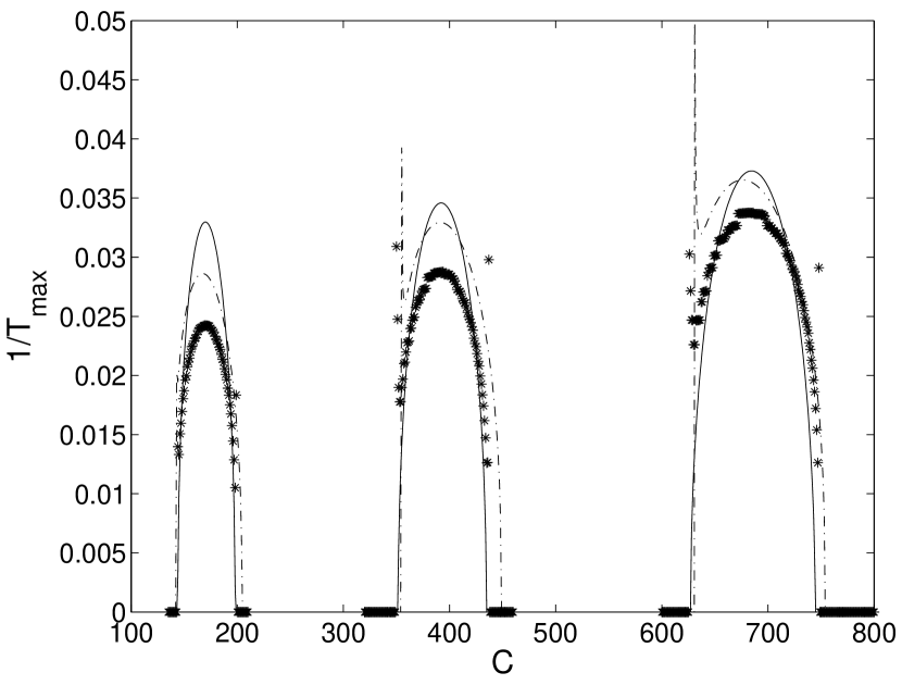
Figure 4: Time for splitting of a doubly quantized vortex. Full lines represent the imaginary part of the complex Bogoliubov eigenvalue, asterisks represent the time $T_{\rm max}$ taken for the vortex distance to achieve its first maximum according to the full GPE solution, and the dashed line is the same time scale in the three-state model, Eq. (83).

The dashed line in Fig. 4 is the result of the three-state model that will be described in Sec. V below. We see that in all instability regions the imaginary part of the mode frequency agrees well with the inverse of $T_{\rm max}$.

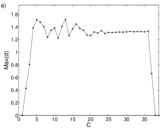
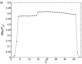
Figure 5: (a) The maximum radius of the motion of the vortices, and (b) the maximum occupation of the $m=0$ state, as a function of coupling parameter C with initial seeding $P_{0}(0)=0.01$. The chosen range of $C$ values lies in the first instability region.

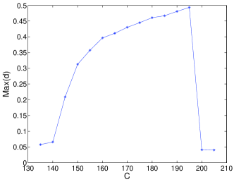
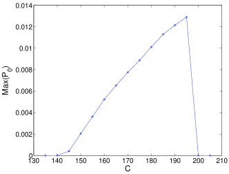
Figure 6: (a) The maximum radius of the motion of the vortices, and (b) the maximum probability of the $m=0$ state, $P_{0}$, as a function of coupling parameter $C$ with initial seeding $P_{0}(0)=0.001$. The chosen range of $C$ values lies in the second instability region.

On the other hand, items (iii) and (iv), the maximum amplitude of the vortex distance and the maximum population of the unstable mode, show a quite surprising behavior. For the first instability region we see in Fig. 5 that both the maximum of the vortex distance and the maximum of the population are approximately independent of $C$ in the unstable region. This is despite that the time to achieve this maximum varies strongly with $C$.

For the higher unstable regions the behavior is very different. We present the result for the region $C\in[135,205]$ in Fig. 6. The behavior of the maximum amplitude is particularly interesting since it has an almost linear increase from the start of the unstable region and reaches a maximum at the strong-coupling end of the unstable region, where it jumps discontinuously to zero. This behavior will be explained in Sec. V, where it is also shown that just outside this discontinuity a finite-amplitude perturbation can bring the system into the unstable region where the amplitude grows approximately to the maximum value achieved at the discontinuity. Finally we note in Fig. 6 that the maximal vortex distance $d$ displays a similar behavior if one takes into account that $P_{0}\sim d^{2}$.

V Three-mode dynamics of vortex splitting

This section is devoted to extracting the main features of the dynamics of the splitting dynamics of the doubly quantized vortex that was studied numerically in the previous section. We put up a nonlinear model that can be solved analytically and which captures the main dynamics of the full system. The parameters of the model can be extracted from the the GP equation, for the most part analytically, and are all functions of $C$. This model will be particularly accurate for the higher unstable regions.

V.1 First instability region

It is instructive to first consider the dynamics in the first unstable region kavoulakis2004 . To find approximative solutions to the the GP equation, it is useful to start from the Lagrangian from which the full GP equation can be derived if no further approximations are invoked Pethick2001 ,

$$L=i\int d{\bf r}\frac{1}{2}({\Psi}^{*}\frac{\partial\Psi}{\partial t}-\Psi\frac{\partial{\Psi}^{*}}{\partial t})-({\Psi}^{*}H_{0}\Psi+\frac{C}{2}|\Psi|^{4}).$$ (18)

In the limit of small $C$, we know that the the dynamics mainly involves three states, namely the lowest-energy harmonic-oscillator eigenstates $\phi_{n,m}=\phi_{0,0}$, $\phi_{0,2}$, and $\phi_{0,4}$ (see Eq. 15). The $m=2$ state represents the condensate, and $m=0$ and $m=4$ the core and surface states respectively, which will be populated due to the instability. To investigate the dynamics of the vortex splitting in the space spanned by the three states, we expand the wave function as

$$\Psi({\bf r},t)=a_{0}(t)\phi_{0,0}({\bf r})+a_{2}(t)\phi_{0,2}+a_{4}(t)\phi_{0,4},$$ (19)

so that $a_{m}$ is the amplitude of the state with $m$ quanta of angular momentum in the $z$-direction. If we insert this into the Lagrangian we obtain

$$L = i\sum_{m}\left(a_{m}^{*}\dot{a}_{m}-\dot{a}^{*}_{m}a_{m}\right)$$ (20)

$$- \sum_{m}\omega_{m}a_{m}^{*}a_{m}-\frac{1}{2}\sum_{m}C_{m,m}(|a_{m}|)^{4}$$

$$- \sum_{m<m^{\prime}}C_{m,m^{\prime}}|a_{m}|^{2}|a_{m^{\prime}}|^{2}$$

$$- K(a_{0}{a_{2}^{2}}^{*}a_{4}+a^{*}_{0}a_{2}^{2}a^{*}_{4})$$

where $C_{m,m^{\prime}}=C\int|\phi_{0,m}|^{2}|\phi_{0,m^{\prime}}|^{2}d^{2}r$, with $m,m^{\prime}=0,2,4$, and $K=C\int|\phi_{0,0}||\phi_{0,2}|^{2}|\phi_{0,4}|d^{2}r$. The angular momentum conservation is automatically taken care of by the symmetries of the eigenfunctions. Using this expression we can write down the nonlinear equations of motion

$$i\dot{a}_{0} = (E_{0}+C_{0,0}|a_{0}|^{2}+C_{0,2}|a_{2}|^{2}+C_{0,4}|a_{4}|^{2})a_{0}+Ka_{2}^{2}a^{*}_{4}$$ (21)

$$i\dot{a}_{2} = (E_{2}+C_{2,0}|a_{0}|^{2}+C_{2,2}|a_{2}|^{2}+C_{2,4}|a_{4}|^{2})a_{2}+2Ka_{0}a^{*}_{2}a_{4}$$ (22)

$$i\dot{a}_{4} = (E_{0}+C_{4,0}|a_{0}|^{2}+C_{4,2}|a_{2}|^{2}+C_{4,4}|a_{4}|^{2})a_{4}+Ka_{0}^{*}a_{2}^{2}.$$ (23)

Making a variable change $a_{m}\to\widetilde{a}_{m}=a_{m}e^{i\theta_{m}(t)}$, with a suitable choice of phases $\theta_{m}$, the system of equations can be rewritten as

$$i\dot{\widetilde{a}}_{0} = K\widetilde{a}_{2}^{2}\widetilde{a}^{*}_{4}e^{i\phi(t)}$$

$$i\dot{\widetilde{a}}_{2} = 2K\widetilde{a}_{0}\widetilde{a}^{*}_{2}\widetilde{a}_{4}e^{-i\phi(t)}$$

$$i\dot{\widetilde{a}}_{4} = K\widetilde{a}^{*}_{0}\widetilde{a}_{2}^{2}e^{i\phi(t)},$$ (25)

where the phase is

$$\phi(t) = \int^{t}(E_{0}+C_{0,0}|a_{0}|^{2}+C_{0,2}|a_{2}|^{2}+C_{0,4}|a_{4}|^{2})$$ (26)

$$+ (E_{4}+C_{4,0}|a_{0}|^{2}+C_{4,2}|a_{2}|^{2}+C_{4,4}|a_{4}|^{2})$$ (27)

$$- 2(E_{2}+C_{2,0}|a_{0}|^{2}+C_{2,2}|a_{2}|^{2}+C_{2,4}|a_{4}|^{2})dt.$$ (28)

It can be seen from Eq. (25), that if initially $\widetilde{a_{0}}(0)=\widetilde{a_{4}}(0)$, then it holds that $\widetilde{a_{0}}(0)=\widetilde{a_{4}}(0)$ at all times.

This equation is expected to give the correct dynamics for small $C$, where the dynamics is dominated by the lowest-energy single-particle eigenfunctions. For larger $C$ values, the structure of the equation is still expected to be the same. As we will see below, the $m=2$ wavefunction should then be replaced by the condensate wavefunction and the $m=0$ and $m=4$ states with the two Bogoliubov states associated with core excitations and surface excitations, respectively.

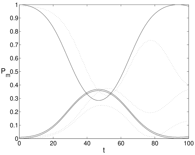
Figure 7: The time dependence of the amplitude of the lowest $m$ states in the truncated three-state model in equation 28, compared to the full GPE simulation. The interaction strength is $C=5$ and the initial seeding $P_{0}=0.1$. From top to bottom, the full lines represent the amplitudes $P_{2}$, $P_{0}$, and $P_{4}$ in the truncated model and the dotted lines represent the corresponding amplitudes for the full GPE simulation.

In Fig. 7 we see that as long as the population is concentrated to the three states used in the truncation, the evolution of the truncated equation is identical to the full solution shown in Fig. 2. The main cause for discrepancies is that the $m=6$ state starts to become populated, which causes a relative depletion of the $m=4$ state. This results in an asymmetry between the populations of the $m=4$ and $m=0$ states, and also implies that the amplitude $a_{0}$ (and with it the vortex distance) will not return back to zero, as it does in the truncated model. The terms in the Lagrangian (18) causing this conversion are of the form $a_{2}a_{4}a_{0}^{*}a_{6}^{*}$ and $a_{4}^{2}a_{2}^{*}a_{6}^{*}$, and thus they are proportional to three powers of the excited-state populations. In situations where the population of all higher states is small, the population of $m=6$ and higher states is expected to be much slower, and this is also seen in Fig. 3; thus a three-state model should be more accurate for higher instability regions than for the first.

The truncated system has six degrees of freedom, corresponding to the real and imaginary parts of the three amplitudes $a_{m}$, but it has to conserve energy, norm and angular momentum, which leaves three degrees of freedom. In addition, the relative phase of the coefficients $\widetilde{a_{0}}$ and $\widetilde{a_{4}}$ will according to Eq. (25) stay constant; thus the system has only two degrees of freedom, which makes it integrable, so that the solution is periodic.

The temporal dynamics depends on the initial state; since the initial increase of the excited-state population is exponential, it is expected that the time taken to achieve the first maximum is proportional to the logarithm of the initial population of the excited states. It is checked numerically that this logarithmic behavior is in fact very accurate even for the full nonlinear evolution.

V.2 Higher instability regions

For the dynamics in the higher unstable regions we have to modify the three-state model so that it takes into account the energy of the condensate and the coupling dependence of the quasiparticle energies. The structure of the model should also be such that it conserves angular momentum, quasiparticles and energy. The ansatz is therefore written

$$\Psi({\bf r},t)=e^{i\mu t}\left[a_{2}(t)\Psi_{2}({\bf r})+a_{0}(t)u_{0}({\bf r})+a_{0}^{*}(t)v_{0}^{*}({\bf r})+a_{4}(t)u_{4}({\bf r})+a_{4}^{*}(t)v_{4}^{*}({\bf r})\right],$$ (29)

where $\Psi_{2}({\bf r})$ is the condensate wavefunction with a doubly quantized vortex, and $u_{0}$ and $v_{0}$ are the Bogoliubov amplitudes for the core mode with $m=0$. Finally, $u_{4}$ and $v_{4}$ are the Bogoliubov amplitudes for a selected quadrupole mode, which is expected to become unstable when it mixes with the core mode. In Ref. Lundh06 it was found that an instability occurs when the energy of the $(n,m)=(0,0)$ Bogoliubov mode, the core mode, becomes nearly degenerate with a quadrupole mode with quantum numbers $(n,m)=(n,m)$; the recurring instability regions arise from the crossings with quadrupole modes with successively higher $n$ values; this can be seen in Fig. 1. All the functions in Eq. (29) are assumed to be calculated from Eqs. (5,7) at some fixed coupling strength $C$ outside of any instability region; their energies are then to be extrapolated into the instability region.

The calculations are carried out in Appendix A. As already noted, the energies of the two Bogoliubov modes are nearly degenerate, and are assumed to coincide at a coupling $C_{0}$. Furthermore, since the core mode is concentrated to the interior of the vortex, its energy varies much more rapidly with coupling strength $C$ than that of the quadrupole mode, so that only the $C$ dependence of the former needs to be taken into account. Again, this is seen in Fig. 1. Moreover, the same confinement also leads to a self-interaction of the core mode; corresponding terms for the other modes are small in comparison. Putting all this together results in the coupled equations

$$i\dot{a}_{0} = (2dE-2I_{0}|a_{0}|^{2})a_{0}+Ka_{2}^{2}a^{*}_{4}$$

$$i\dot{a}_{2} = 2Ka_{0}a^{*}_{2}a_{4}$$

$$i\dot{a}_{4} = Ka^{*}_{0}a_{2}^{2}.$$ (30)

Here, $dE=(\omega_{0}-\omega_{4})/2$ is half the $C$-dependent energy difference between the Bogoliubov eigenenergies; at the resonant coupling strength $C_{0}$ we have $2dE(C_{0})=\omega_{0}(C_{0})-\omega_{4}=0$, so we may write

$$dE=\frac{1}{2}\frac{\partial\omega_{0}}{\partial C}(C-C_{0}).$$ (31)

Inserting the 2D Thomas-Fermi approximation Pethick2001 $\mu(C)=(C/\pi)^{1/2}$, and using the expression for the core mode energy Lundh06 , $\omega=0.42\mu$, we obtain

$$dE=0.42\frac{1}{2\sqrt{\pi C_{0}}}(C-C_{0}).$$ (32)

The term $I_{0}$ in Eq. (30) represents the nonlinear self-interaction of the core mode,

$$I_{0}=\frac{1}{2}C\int d{\bf r}|v_{0}|^{4}({\bf r})\approx\frac{C_{0}^{3/2}}{4\sqrt{3}\pi^{3/2}},$$ (33)

where the last equality was carried out in App. A. With Thomas-Fermi estimates for the core mode frequency Lundh06 ,

$$\omega_{0}(C)=0.42\sqrt{\frac{C}{\pi}},$$ (34)

and the quadrupole mode frequency for the $n$’th radially excited state stringari ,

$$\omega_{4}=\sqrt{2n^{2}+6n+2},$$ (35)

the resonant coupling $C_{0}$ was obtained in Ref. Lundh06 as

$$C_{0}=\frac{\pi}{0.42^{2}}(2n^{2}+6n+2),$$ (36)

where each value of $n$ corresponds to an instability region. Finally, the constant $K$ represents the integral that couples the three modes; it is found that any attempt to approximate this term analytically is extremely sensitive to small variations in the variational parameters, so $K$ has to be determined numerically. This can be done by noting (as will be shown in a moment) that the constant is fact equal to the maximum of the imaginary parts of the mode frequencies over the instability interval; numerically it is seen to be close to $K\approx 0.15$ for all instability regions. We note that $I_{0}$ is at least an order of magnitude larger than $K$ when $C$ is of order 100 or more; this inequality will be taken advantage of in the calculations. Also note that whereas $K$ and $I_{0}$ are positive as long as the interactions are repulsive, the sign of $dE$ depends on $C-C_{0}$.

To see that $K$ is related to the maximum imaginary part of the mode frequency, linearize Eq. (30) by removing the term proportional to $I_{0}$ and put $|a_{2}|=1$; the resulting oscillating solution for the amplitudes $a_{0}$ and $a_{4}$ has a frequency

$$\omega_{\rm lin}=dE\pm\sqrt{dE^{2}-K^{2}}$$ (37)

in accordance with Bogoliubov theory. From this we conclude that the mode is unstable when $|K/dE|<1$, and that $K$ is indeed the maximum imaginary part of the frequency.

In Appendix B it is shown how the system of equations (30) leads to the differential equation for the core mode population $p=|a_{0}|^{2}$,

$$\dot{p}^{2}=-\left[2(dE-K)p-(I_{0}-4K)p^{2}-E_{0}\right]\left[2(dE+K)p-(I_{0}+4K)p^{2}-E_{0}\right]\equiv f(p),$$ (38)

where the constant $E_{0}$ is the total energy. A formal solution is

$$\int_{p(0)}^{p(t)}\frac{{\rm d}p}{\sqrt{f(p)}}=t.$$ (39)

This is an elliptic integral since $f(p)$ is a polynomial of degree 4. The solution for $p(t)$ is therefore given as an inverse of this elliptic integral. To understand the dynamics of the system we look at the zeros of $f(p)$. The solution will oscillate between the two positive roots of $f(p)$, since they correspond to $\dot{p}=0$. In the limit $E_{0}\ll(K,dE)\ll I_{0}$ [which holds according to the discussion below Eq. (36)], the roots can be written

$$p_{0} = \frac{E_{0}I_{0}}{2(K+dE)^{2}},$$

$$p_{\mathrm{m}ax} = 2\frac{dE+K}{I_{0}}-p_{0}.$$ (40)

In a typical experimental situation, $p_{0}$ is the initial value.

In App. C it is found that the asymptotic expansion for the time to the first maximum, under the inequalities stated above, is given by

$$T \sim \frac{1}{4\sqrt{K^{2}-dE^{2}}}\ln\left(\frac{16}{k^{\prime 2}}\right),$$

$$k^{\prime 2} \approx \frac{1}{4(1-(\frac{dE}{K})^{2})^{2}}\frac{I_{0}^{2}}{(K+dE)^{2}}p_{0}^{2}.$$ (41)

The time scale is set by the imaginary part of the eigenvalue of the linearized problem, $\sqrt{K^{2}-dE^{2}}$, as long as we have $|dE/K|<1$, as discussed in connection with Eq. (37). The contribution of the initial population is only logarithmic. The nonlinearity described by the constant $I_{0}$ also contributes a logarithmic term. We conclude that the splitting time is mainly predicted by the linear Bogoliubov theory, and the nonlinear dynamics contributes only weakly.

To further understand the dynamics is is useful to examine the Hamiltonian associated with these equations of motion. It is given by Eq. (68) as

$$H(\psi_{d},p)=2K(\frac{1}{2}-p)p\cos\psi_{d}+(2dE-I_{0}p)p,$$ (42)

where $\psi_{d}$ is twice the phase difference between the two modes $a_{2}$ and $a_{0}$, $\psi_{d}=2\psi_{2}-2\psi_{0}$. Again, we can according to Eqs. (32-33) take the physically motivated limit $K/I_{0}\ll 1$. In Fig. 8 we see a contour plot of the Hamiltonian.

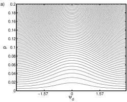
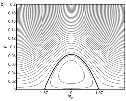
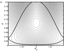
Figure 8: Contour plots of the Hamiltonian (68) for $dE=-1.5$ (a), $dE=0$ (b), and $dE=1.5$ (c). The other parameters are chosen as $I_{0}=10$ and $K=1$. The thick line is the separatrix, dividing phase space into running and oscillating solutions.

Fig. 8(a) shows the case $dE<-K$, where $p=0$ is a global maximum and the Hamiltonian is strictly convex, i.e., $p=0$ is unconditionally stable. In the linearly unstable regime, $K>|dE|$ [Fig. 8(b)], the point $p=0$ is a saddle point and the Hamiltonian has a global maximum for $p=(dE+K)/I_{0},\psi_{d}=0$. The thick line in Fig. 8 is the separatrix, separating the solutions where $\psi_{d}$ oscillates from the running ones. Finally, for $dE>K$, as shown in (c), $p=0$ is a local minimum and the Hamiltonian has a saddle point at $p=(dE-K)/I_{0}$ and $\psi_{d}=\pi$. In this case the solution is stable when the initial conditions are sufficiently near $p=0$; else it may start to oscillate around the maximum.

The zeros of the polynomial $f(p)$ defined in Eq. (38) correspond to points where the tangent of a contour line is horizontal. We observe that the contours are of two different types depending on whether they are closed lines, that do not wind about the origin, or whether they wind around phase space and connect at $\psi_{d}=\pm\pi$. If the initial condition is purely imaginary, $\psi_{d}=\pi$, then the solution will always lie on a curve that winds around phase space. In the case $\psi_{d}=0$ the solution can lie on any level curve depending on the initial condition. Consider the case where $dE>K$, i.e., $C$ is above the unstable region. Then a small initial value of $p$ will yield a solution that lies in the stable region, i.e. the solution will circle around the local maximum. However, if the initial value of $p$ is increased, the system enters a trajectory that winds around the minimum and $p$ starts to oscillate. This is the reason for the finite-amplitude instabilities above the upper limit of the unstable region that were observed numerically in Sec. IV.

In Figs. 9-10 and Fig. 4 we compare the three-state model calculation with the full time integration.

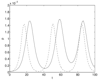
Figure 9: Time development of the population $p$ of the core mode. Full line represents the full numerical time integration, while the dashed line is obtained from the three-state approximation. The coupling strength is chosen as $C=380$.

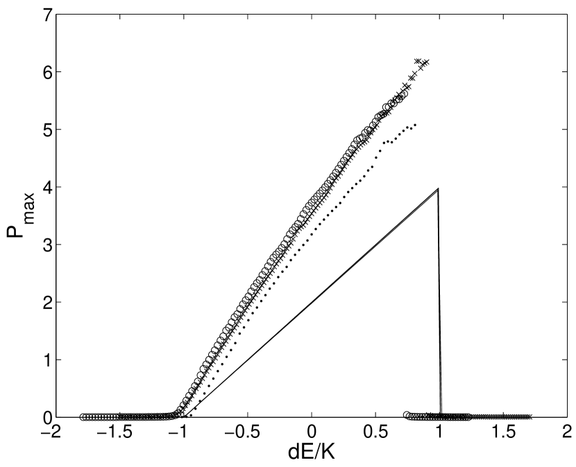
Figure 10: Maximum amplitude $p_{0}$ of the core mode as a function of energy difference divided by mode coupling, $dE/K$. The full line is the analytical solution of the three-state model, and the symbols represent data from the GPE solution in successive instability regions; circles for the second instability region, crosses for the third, and dots for the fourth.

The overlap $p$ is in the numerical calculation defined as the overlap integral between the condensate wave function and the core mode, analogously to Eq. (14), but with the numerically calculated core mode $v_{0}$ substituted for the single-particle eigenfunction $\phi_{0,0}$. Fig. 10 collapses numerical data from the solution of the GP equation in several instability regions onto the same graph, by for each instability region mapping the coupling parameter $C$ onto the parameters $dE$ and $K$. As seen, the agreement with the three-state model for the time $T$ in Fig. 4 is excellent, but the magnitude of the amplitude $p$, seen in Fig. 10, is more sensitive to the exact parameter values, which may explain the discrepancy by a factor of order unity. Again, $p$ does not oscillate back to zero in the full solution, but it does in the truncated model. Clearly, the population of higher states makes the dynamics nonperiodic, so that the two vortices stay apart after they have separated.

VI Conclusions

This study is concerned with the compressible vortex dynamics in a trapped Bose-Einstein condensate. The dynamics of the splitting of a doubly quantized vortex is studied in detail both in full numerical time integration, linear Bogoliubov analysis, and using a three-state model utilizing the Bogoliubov eigenstates. It is found that the simple three-state model captures many essential features of the dynamics. Moreover, it is seen that Bogoliubov analysis is capable of determining the time scale for vortex splitting, while nonlinear processes only contribute logarithmically.

VII Acknowledgment

Part of this work was supported by the Swedish research council, Vetenskapsrådet.

Appendix A Derivation of three-state model

We start from the ansatz

$$\Psi({\bf r},t)=e^{-i\mu t}\left[a_{2}(t)\Psi_{2}({\bf r})+a_{0}(t)u_{0}({\bf r})+a_{0}^{*}(t)v_{0}^{*}({\bf r})+a_{4}(t)u_{4}({\bf r})+a_{4}^{*}(t)v_{4}^{*}({\bf r})\right],$$ (43)

where $u_{m},v_{m}$ are the exact Bogoliubov amplitudes associated with the stationary condensate wave function $\Psi_{2}$ computed for a nonlinearity parameter $C$. $C$ is assumed to lie outside of all instability regions, and the energies will be extrapolated into them. The dimensionless units were discussed in connection with Eq. (4). We assume that the core state can be approximated well as a pure hole state. This assumption amounts to putting $u_{0}=0$. The functions thus fulfill the equations

$$\int d{\bf r}\Psi^{*}_{2}({\bf r})(H_{0}+C|\Psi_{2}({\bf r})|^{2})\Psi_{2}({\bf r}) = \mu,$$

$$\int d{\bf r}v^{*}_{0}({\bf r})(H_{0}+2C|\Psi_{2}({\bf r})|^{2}-\mu)v_{0}({\bf r}) = -\omega_{0}(C),$$

$$\int d{\bf r}u^{*}_{4}({\bf r})[(H_{0}+2C|\Psi_{2}({\bf r})|^{2}-\mu)u_{4}({\bf r})+C\Psi_{2}^{2}({\bf r})v_{4}({\bf r})]-$$

$$\int d{\bf r}v^{*}_{4}({\bf r})[(H_{0}+2C|\Psi_{2}({\bf r})|^{2}-\mu)v_{4}({\bf r})+C(\Psi^{*}_{2})^{2}u_{4}({\bf r})] = \omega_{4}(C).$$ (44)

With the chosen sign conventions, $\omega_{0}$ and $\omega_{4}$ are both positive. In the absence of instabilities, $a_{4}$ is expected to oscillate as $\exp(-i\omega_{4}t)$, and $a_{0}$ oscillates as $\exp(-i\omega_{0}t)$. Taking nonlinearities into account, there will of course be corrections to the time dependence. Also note the dependencies on the azimuthal angle $\theta$: $\Psi_{2}\propto\exp(2i\theta)$, $u_{4}\propto\exp(4i\theta)$, but $v_{0}$ and $v_{4}$ do not depend on $\theta$.

On inserting the ansatz (43) into the Lagrangian (18), it separates into five parts,

$$L=L_{k}+L_{0}+L_{r}+L_{2}+L_{4},$$ (45)

where $L_{k}$ contains the time derivatives,

$$L_{k} = \frac{i}{2}({a}^{*}_{0}\dot{a}_{0}+{a}^{*}_{2}\dot{a}_{2}+{a}^{*}_{4}\dot{a}_{4}-c.c.)$$ (46)

$$+\frac{i}{2}(a_{0}\dot{a_{4}}\int d{\bf r}v_{0}({\bf r}){v}^{*}_{4}({\bf r})-c.c.).$$

The term $L_{0}$ contains the terms to which the eigenvalue equations (44) can be applied,

$$L_{0} = -|a_{2}|^{2}\int d{\bf r}\left[\mu|\Psi_{2}({\bf r})|^{2}-\Psi^{*}_{2}({\bf r})(H_{0}+C|\Psi_{2}({\bf r})|^{2})\Psi_{2}({\bf r})\right]$$ (47)

$$-|a_{0}|^{2}\int d{\bf r}v_{0}({\bf r})(H_{0}+2C|\Psi_{2}({\bf r})|^{2}-\mu)v^{*}_{0}({\bf r})$$

$$-|a_{4}|^{2}\int d{\bf r}\left[u^{*}_{4}({\bf r})(H_{0}+2C|\Psi_{2}({\bf r})|^{2}-\mu)u_{4}({\bf r})\right.$$

$$\left.+v_{4}({\bf r})(H_{0}+2C|\Psi_{2}({\bf r})|^{2}-\mu)v^{*}_{4}({\bf r})\right],$$

whereas $L_{r}$ collects the “rest terms” obtained from $L_{0}$ because of the depletion of the condensate,

$$L_{r} = -C\,|a_{2}|^{2}(\frac{|a_{2}|^{2}}{2}-1)\int d{\bf r}|\Psi_{2}({\bf r})|^{4}$$ (48)

$$-2C|a_{0}|^{2}(|a_{2}|^{2}-1)\int d{\bf r}|\Psi_{2}({\bf r})|^{2}|v_{0}({\bf r})|^{2}$$

$$-2C|a_{4}|^{2}(|a_{2}|^{2}-1)\int d{\bf r}|\Psi_{2}({\bf r})|^{2}|u_{4}({\bf r})|^{2}$$

$$-2C|a_{4}|^{2}(|a_{2}|^{2}-1)\int d{\bf r}|\Psi_{2}({\bf r})|^{2}|v_{4}({\bf r})|^{2}.$$

The term $L_{2}$ contains terms of second order in the excited-state amplitudes,

$$L_{2} = -C[{a}^{*}_{0}a^{*}_{4}(a_{2})^{2}\int d{\bf r}\Psi_{2}({\bf r})^{2}v^{*}_{0}({\bf r})u^{*}_{4}({\bf r})+c.c.]$$ (49)

$$-Ca_{0}a^{*}_{4}|a_{2}|^{2}\int d{\bf r}|\Psi_{2}({\bf r})|^{2}v_{0}({\bf r})v_{4}({\bf r})$$

$$-C[|a_{4}|^{2}|a_{2}|^{2}\int d{\bf r}\Psi_{2}({\bf r})^{2}u^{*}_{4}({\bf r})v_{4}({\bf r})+c.c.],$$

and analogously, $L_{4}$ contains the fourth-order terms,

$$L_{4} = -\frac{C}{2}|a_{0}|^{4}\int d{\bf r}|v_{0}({\bf r})|^{4}$$ (50)

$$-\frac{C}{2}|a_{4}|^{2}\int d{\bf r}(|u_{4}({\bf r})|^{4}+|v_{4}({\bf r})|^{4})$$

$$-C|a_{0}|^{2}|a_{4}|^{2}\int d{\bf r}|v_{0}|^{2}(|v_{4}|^{2}+|u_{4}|^{2})$$

$$-C|a_{4}|^{4}\int d{\bf r}|v_{4}({\bf r})|^{4}|u_{4}({\bf r})|^{2}.$$

All the terms that are expected to oscillate as $\exp[i(\omega_{0}+\omega_{4})t]$ are discarded. Next, consider all terms that are proportional to the fourth power of the excited-state amplitudes. Note that the function $v_{0}$ is concentrated to the vortex core, i.e., a very small spatial region, while the other functions, $\Psi_{2}$, $u_{4}$, and $v_{4}$, are much less localized. As a result, the term in the first line in Eq. (50) is expected to be much larger than all the other terms in $L_{4}$, and those are therefore discarded. Furthermore, all the terms in $L_{r}$ are also of fourth order in the excited-state amplitudes and can be discarded. The resulting Lagrangian is

$$L = \frac{i}{2}({a}^{*}_{0}{\dot{a}}_{0}+{a}^{*}_{4}\dot{a}_{4}+{a}^{*}_{2}\dot{a}_{2}-c.c.)$$ (51)

$$- |a_{0}|^{2}\omega_{0}(C)-|a_{4}|^{2}\omega_{4}(C)$$

$$- C\left(a_{0}a_{4}(a^{*}_{2})^{2}\int d{\bf r}u_{4}v_{0}|\Psi_{2}|^{2}+c.c.\right)$$

$$- \frac{C}{2}|a_{0}|^{4}\int d{\bf r}|v_{0}({\bf r})|^{4}.$$

Defining the constants

$$K=C\int d{\bf r}u_{4}v_{0}|\Psi_{2}|^{2},$$

$$I_{0}=\frac{1}{2}C\int v_{0}^{4},$$

$$dE=\frac{1}{2}[\omega_{0}(C)-\omega_{4}(C)],$$ (52)

and making a phase change we can write the Lagrangian on the final form

$$L = \frac{i}{2}({a}^{*}_{0}{\dot{a}}_{0}+{a}^{*}_{4}\dot{a}_{4}+{a}^{*}_{2}\dot{a}_{2}-c.c.)$$ (53)

$$- 2dE|a_{0}|^{2}-I_{0}|a_{0}|^{4}-\left(Ka_{0}a_{4}(a^{*}_{2})^{2}+c.c.\right).$$

Following Ref. Lundh06 , one may produce Thomas-Fermi estimates for $I_{0}$ and $dE$, assuming that the core mode experiences an effective potential

$$V(r)=2C|\Psi|^{2}=2\mu\frac{r^{2}}{\xi^{2}b^{2}}$$ (54)

where $\xi=1/\sqrt{2\mu}$ is the healing length, and $b$ is a variational parameter; the choice $b=2\sqrt{6}$ minimizes the condensate energy. The ground state of this potential is

$$v_{0}(r)=\sqrt{\frac{\mu}{\pi\sqrt{3}}}\exp(-\frac{\mu}{\sqrt{3}}\frac{r^{2}}{2}),$$ (55)

and the nonlinear parameter of our model becomes

$$I_{0}=\frac{C}{2}\frac{\mu}{\sqrt{3}}\frac{1}{2\pi}=\frac{C^{3/2}}{4\sqrt{3}\pi^{3/2}},$$ (56)

where in the last line we used the Thomas-Fermi result $\mu=(C/\pi)^{1/2}$.

Appendix B Solution of the coupled nonlinear system

The Lagrangian for the system was in App. A found to be

$$L({a_{m}},{a^{*}_{m}})=\sum_{m}\frac{i}{2}\left(a^{*}_{m}\dot{a}_{m}-{a_{m}}\dot{a}^{*}_{m}\right)-\left[(2dE-I_{0}|a_{0}|^{2})|a_{0}|^{2}+K\left((a_{2}^{*})^{2}a_{0}a_{4}+a_{2}^{2}a^{*}_{0}a^{*}_{4}\right)\right].$$ (57)

First write the amplitudes in the form $a_{i}=r_{i}\exp(i\psi_{i})$. The Lagrangian can then be written in the form

$$L({r_{m}},{\psi_{m}})=\sum_{m}\dot{\psi}_{m}r^{2}_{m}-\left\{2Kr_{2}^{2}r_{0}r_{4}\cos[2\psi_{2}-(\psi_{0}+\psi_{4})]+(2dE-I_{0}r_{0}^{2})r_{0}^{2}\right\}.$$ (58)

Defining the auxiliary variables

$$N = r_{0}^{2}+r_{2}^{2}+r_{4}^{2},\quad\psi_{n}=2\psi_{2}-2\psi_{4},$$

$$L = 2r_{2}^{2}+4r_{4}^{2},\quad\psi_{l}=\frac{1}{4}(\psi_{4}-\psi_{0}),$$

$$D = r_{0}^{2}+\frac{1}{2}r_{2}^{2}+r_{4}^{2},\quad\psi_{d}=-2\psi_{2}+\psi_{0}+\psi_{4},$$ (59)

the Lagrangian can be rewritten once more as

$$L(N,L,D,\psi_{n},\psi_{l},\psi_{d})=\dot{\psi}_{n}N+\dot{\psi_{l}}L+\dot{\psi}_{d}D-\sqrt{F(D)}\cos\psi_{d}+G(D),$$ (60)

where

$$F(D) = 4K^{2}(2N-2D)^{2}(D-L/4)(-N+L/4+D),$$

$$G(D) = [2dE-I_{0}(D-L/4)](D-L/4).$$ (61)

We see that $N$ and $L$ are conserved; they are in fact the norm and angular momentum, respectively, so we suppress them as arguments. In addition the energy function

$$E=\sqrt{F(D)}\cos\psi_{d}+G(D)$$ (62)

is conserved. The Lagrange equations for $D$ and $\psi_{d}$ read

$$\dot{D} = -\sqrt{F(D)}\sin\psi_{d},$$

$$\dot{\psi_{d}} = \frac{\partial}{\partial D}\sqrt{F(D)}\cos\psi_{d}+\frac{\partial}{\partial D}G(D).$$ (63)

Using energy conservation and the square of the first line we obtain the ODE

$$\dot{D}^{2}=F(D)-(E-G(D))^{2}.$$ (64)

This is an elliptic ODE since the right hand side is a polynomial of degree $4$. The solution is done by factorizing the polynomial on the right-hand side into two second-order polynomials.

Suppose $N=1$, $L=2$, which is the case in the present physical problem. In this case $F(D)$ is a square,

$$F(D)=f(D)^{2}\equiv 4K^{2}(1-D)^{2}(D-\frac{1}{2})^{2},$$ (65)

and the equation (64) for $D$ simplifies to

$$\dot{D}^{2} = (f(D)+E-G(D))(f(D)-(E-G(D))).$$ (66)

Now rewrite the equation in terms of the original variable $p=r_{0}^{2}$ and obtain the final equation of motion,

$$\dot{p}^{2} = P_{1}(p)P_{2}(p),{\rm where}$$

$$P_{1}(p) = (-4K+I_{0})p^{2}+2(K-dE)p+E,$$

$$P_{2}(p) = (-4K-I_{0})p^{2}+2(K+dE)p-E.$$ (67)

Note that the roots of the polynomial $P_{1}(p)P_{2}(p)$ may be either real or complex; two roots will become complex when $(dE-K)^{2}<(I_{0}-4K)E$. Since $E$ is proportional to the initial population $p_{0}$ [see Eq. (40)], it can be assumed small and hence the complex roots appear only in a very small portion of phase space; this permits us to concentrate on the case with real roots only. Furthermore, as is shown in Sec. V, we can on physical grounds assume $I_{0}\gg K$; this will simplify some expressions in the following.

It is useful to write these equations as a Hamiltonian system with $\psi_{d},p$ canonically conjugate variables. Starting from Eqs. (63) for $\psi_{d},D$ and shifting variables as above to $\psi_{d},p$ we obtain

$$H(\psi_{d},p)=2K(\frac{1}{2}-p)p\cos\psi_{d}+(2dE-I_{0}p)p.$$ (68)

Appendix C Elliptic integrals

We now solve the differential equation for the core-mode amplitude $p$, Eq. (67). Rewriting this as

$$\dot{p}=I_{0}\sqrt{(p-p_{\rm min})(p+p_{1})(p_{\rm max}-p)(p_{2}+p)},$$ (69)

where $p_{\rm min}$ and $p_{\rm max}$ are the smallest and largest positive roots of the polynomial, respectively, and $-p_{1}$ and $-p_{2}$ are the other two, and taking the initial value for $p$ to be at the minimum point, then we may write

$$t=\frac{1}{I_{0}}\int_{p_{\rm min}}^{p(t)}\frac{dp}{[(p-p_{\rm min})(p+p_{1})(p_{\rm max}-p)(p_{2}+p)]^{1/2}}.$$ (70)

Now define $p_{l}=(p_{\rm min}+p_{1})/2$,$dl=(p_{\rm min}-p_{1})/2$, $p_{b}=(p_{\rm max}+p_{2})/2$, $db=(p_{\rm max}-p_{2})/2$, and $p^{\prime}=p-dl$, to obtain the integral

$$t=\frac{1}{I_{0}}\int_{p_{l}}^{p^{\prime}(t)}\frac{dp^{\prime}}{[(p^{\prime 2}-p_{l}^{2})((p_{b}+db-dl)-p^{\prime})((p_{b}-db-dl)+p^{\prime})]^{1/2}}.$$ (71)

The asymmetry between the largest zeros can be removed by invoking the substitution (Whittaker35 , p. 514)

$$p^{\prime}=\frac{ax+b}{cx+d}.$$ (72)

The parameters are to be determined so that the transformation leaves the symmetric zeros of the integrand invariant but makes the other two symmetric in terms of the new variable $x$; the new zeros of the denominator are denoted by $\pm p_{s}$. The integral for $t$ is now

$$t = \frac{A}{I_{0}}\int_{p_{l}}^{x(t)}\frac{dx}{\sqrt{(x^{2}-p_{l}^{2})(p_{s}^{2}-x^{2})}},$$ (73)

and assuming that all roots are real, as discussed in App. B, the solution is

$$\frac{I_{0}p_{s}}{A}t = {\rm nd}^{-1}\left(\frac{x(t)}{p_{l}},1-\left(\frac{p_{l}}{p_{s}}\right)^{2}\right),$$ (74)

where ${\rm nd}$ is a Jacobian elliptic function (Abramowitz72 , p.596), and

$$A^{2}=\frac{(ad-cd)^{2}}{((ap_{l})^{2}-c^{2})(c-(a(p_{b}+dr)))(c+a(p_{b}-dr))},$$ (75)

with $dr=db-dl$. This gives the complete result

$$x(t) = p_{l}\,{\rm nd}(\frac{I_{0}p_{s}}{A}t),$$

$$p(t) = \frac{ax(t)+b}{cx(t)+d}+dl.$$ (76)

The half period $T$ of the function $p(t)$ is given by the complete elliptic integral

$$T=\frac{A}{I_{0}p_{s}}{\cal K}(k^{\prime 2}),\quad k^{\prime 2}=(\frac{p_{l}}{p_{s}})^{2}.$$ (77)

Expanding the parameters in powers of $p_{l}$, which in our physical situation corresponds to assuming that the initial population is very small, yields

$$A^{2} \approx (1-(\frac{dr}{p_{b}})^{2})-\frac{dr^{2}}{p_{b}^{2}}\frac{1}{(1-\frac{dr}{p_{b}})}\frac{p_{l}^{2}}{p_{b}^{2}}+{\mathcal{O}}(p_{l}^{4}).$$ (78)

The transformation is given by

$$d = a\approx c\left(\frac{dr^{2}-p_{b}^{2}}{dr}-\frac{p_{b}^{2}}{dr(dr^{2}-p_{b}^{2})}p_{l}^{2}+{\mathcal{O}}(p_{l}^{4})\right),$$

$$b = cp_{l}^{2}.$$ (79)

Finally, the transformed root is

$$p_{s}=\frac{p_{b}^{2}-dr^{2}}{p_{b}}+\frac{p_{b}^{2}}{p_{b}(p_{b}^{2}-dr^{2})}p_{l}^{2}+{\mathcal{O}}(p_{l}^{4}).$$ (80)

The asymptotic expression for the complete elliptic integral when its argument is small is

$${\cal K}(k^{\prime})\sim\frac{1}{2}\ln\left(\frac{16}{k^{\prime 2}}\right).$$ (81)

Wrapping up all of the above, we obtain the full time evolution $p(t)$ from Eq. (76) where we substitute

$$A^{2} = 1-(\frac{dE}{K})^{2},$$

$$p_{s} = \frac{2K}{I_{0}}(1-(\frac{dE}{K})^{2}),$$ (82)

and $p_{0}$ is the initial population; the time taken to attain the first maximum is given by

$$T=\frac{1}{4K\sqrt{1-(\frac{dE}{K})^{2}}}\ln\left(\frac{16}{k^{\prime 2}}\right),$$ (83)

where

$$k^{\prime 2}\approx\frac{1}{(1-(\frac{dE}{K})^{2})^{2}}\frac{I_{0}^{2}}{4(K+dE)^{2}}p_{0}^{2}.$$ (84)

References

- (1) U. Essmann and H. Träuble, Phys. Lett. 24A, 526 (1967).
- (2) W. F. Vinen, Proc. Roy. Soc. London A 260, 218 (1960).
- (3) K. W. Madison, F. Chevy, W. Wohlleben, and J. Dalibard, Phys. Rev. Lett. 84, 806 (2000).
- (4) C. Raman, J. R. Abo-Shaeer, J. M. Vogels, K. Xu, and W. Ketterle, Phys. Rev. Lett. 87, 210402 (2001); J.R. Abo-Shaeer, C. Raman, J.M. Vogels, and W. Ketterle, Science 292, 476 (2001).
- (5) C. J. Pethick and H. Smith, Bose-Einstein Condensation in Dilute Gases (Cambridge University Press, Cambridge, 2001).
- (6) D. A. Butts and D. S. Rokhsar, Nature 397, 327 (1999).
- (7) Emil Lundh, Phys. Rev. A 65, 043604 (2002).
- (8) M. Möttönen, T. Mizushima, T. Isoshima, M. M. Salomaa, and K. Machida, Phys. Rev. A 68, 023611 (2003).
- (9) H. Pu, C. K. Law, J. H. Eberly, and N. P. Bigelow, Phys. Rev. A 59, 1533 (1999).
- (10) A. D. Jackson, G. M. Kavoulakis, and E. Lundh, Phys. Rev. A 72, 053617 (2005).
- (11) Y. Shin, M. Saba, M. Vengalattore, T. A. Pasquini, C. Sanner, A. E. Leanhardt, M. Prentiss, D. E. Pritchard, and W. Ketterle, Phys. Rev. Lett. 93, 160406 (2004).
- (12) J. A. M. Huhtamäki, M. Möttönen, T. Isoshima, V. Pietilä, and S. M. M. Virtanen, Phys. Rev. Lett. 97, 110406 (2006).
- (13) A. M. Mateo and V. Delgado, Phys. Rev. Lett. 97, 180409 (2006).
- (14) J. A. M. Huhtamäki, M. Möttönen, and S. M. M. Virtanen, Phys. Rev. A 74, 063619 (2006).
- (15) Emil Lundh and Halvor M. Nilsen, Phys. Rev. A 74, 063620 (2006).
- (16) Halvor M. Nilsen, Gordon Baym, and C. J. Pethick, PNAS 103, 7978 (2006).
- (17) W. Thomson (Lord Kelvin), Proc. Roy. Soc. (Edinburgh), 6, 94 (1867).
- (18) D. McPeake, H. M. Nilsen, and J. F. McCann, Phys. Rev. A 65, 063601 (2002).
- (19) A similar analysis was first carried out by G. M. Kavoulakis (unpublished, 2004).
- (20) S. Stringari, Phys. Rev. A 58, 2385 (1998).
- (21) E. T. Whittaker and G. N. Watson, A course of Modern Analysis (Cambridge at the University Press, 1935).
- (22) M. Abramowitz and I. A. Stegun, eds. Handbook of Mathematical Functions with Formulas, Graphs, and Mathematical Tables. (New York: Dover, 1972).