Spectroscopic analysis of finite size effects around a Kondo quantum dot

Abstract

We consider a simple setup in which a small quantum dot is strongly connected to a finite size box. This box can be either a metallic box or a finite size quantum wire. The formation of the Kondo screening cloud in the box strongly depends on the ratio between the Kondo temperature and the box level spacing. By weakly connecting two metallic reservoirs to the quantum dot, a detailed spectroscopic analysis can be performed. Since the transport channels and the screening channels are almost decoupled, such a setup allows an easier access to the measure of finite-size effects associated with the finite extension of the Kondo cloud.

I Introduction

The Kondo effect occurs as soon a magnetic impurity is coupled to a Fermi sea. It is characterized by a narrow resonance of width $T_{K}^{0}$, the Kondo temperature, pinned at the Fermi energy $E_{F}$ hewson . This resonance is related to the many-body singlet state which is formed between the impurity spin and the spin of an electron belonging to a cloud of spin-correlated electrons. This cloud of electrons has been termed as the so-called Kondo screening cloud. The Kondo screening cloud length is therefore related to the spatial extension of this multi-electronic, spin-correlated, wave function. The size of this screening cloud may be evaluated as $\xi_{K}^{0}\approx\hbar v_{F}/T_{K}^{0}$ where $v_{F}$ is the Fermi velocity. Nonetheless, the Kondo screening cloud has never been detected experimentally and has therefore remained a rather elusive prediction.

However, the remarkable recent achievements in nano-electronics may offer new possibilities to finally observe this Kondo cloud. Indeed, the Kondo effect appears as a rather robust and versatile phenomenon. It has been observed by various groups in a single semi-conductor quantum dot dot ; Cronenwett ; simmel ; Wiel , in carbon nanotubes quantum dots cobden ; bachtold ; jarillo , in molecular transistors molecular to list a few. In this respect, the observation of the Kondo effect may be regarded as a test of quantum coherence of the nanoscopic system under study. One of the main signatures of the Kondo effect is a zero-bias anomaly and the conductance reaching the unitary limit $2e^{2}/h$ at low enough temperature $T<T_{K}^{0}$.

In a semi-conducting quantum dot, the typical Kondo temperature is of order $1~{}K$ which leads to $\xi_{K}^{0}\approx 1$ micron in semiconducting heterostructures. Finite size effects (FSE) related to the actual extent of this length scale have been predicted recently in different geometries: an impurity embedded in a finite size box thimm ; monien , a quantum dot embedded in a ring threaded by a magnetic flux affleck01 ; Hu ; sorensen04 ; simon05 , a quantum dot embedded between two open finite size wires (OFSW) (by open we mean connected to at least one external infinite lead) simon02 ; balseiro and also around a double quantum dot simon05b . In the ring geometry, it was shown that the persistent current induced by a magnetic flux is particularly sensitive to screening cloud effects and is drastically reduced when the circumference of the ring becomes smaller than $\xi_{K}^{0}$ affleck01 . In the wire geometry, a signature of the finite size extension of the Kondo cloud was found in the temperature dependence of the conductance through the whole system simon02 ; balseiro . More specifically, in a one-dimensional geometry where the finite size $l$ is associated to a level spacing $\Delta\sim\hbar v_{F}/l$, the Kondo cloud fully develops if $\xi_{K}^{0}\ll l$, a condition equivalent to $T_{K}^{0}\gg\Delta$. On the contrary, FSE effects appear if $\xi_{K}^{0}>l$ or $T_{K}^{0}<\Delta$. In a one dimensional geometry, one can equivalently use the ratio $\xi_{K}^{0}/l$ or $\Delta/T_{K}^{0}$. In higher dimensions, we should rather use the latter ratio or introduce another typical box length scale monien . In the aforementioned two-terminal geometry, the screening of the artificial spin impurity is done in the OFSWs which are also used to probe transport properties through the whole system. This brings at least two main drawbacks: first, the analysis of FSE relies on the independent control of the two wire gate voltages and also a rather symmetric geometry. This is rather difficult to achieve experimentally. In order to remedy to these drawbacks, we propose and study here a simpler setup in which the screening of the impurity occurs mainly in one larger quantum dot or metallic box or OFSW and the transport is analyzed by help of one or two weakly coupled leads. In practice, a lead weakly coupled to the dot by a tunnel junction allows a spectroscopic analysis of the dot local density of states (LDOS) in a way very similar to a STM tip.

The geometry we study is depicted in Fig. 1. We note that this geometry has also been proposed by Oreg and Goldhaber-Gordon oreg to look for signatures of the two-channel Kondo fixed point or by Craig et al. craig to analyze two quantum dots coupled to a common larger quantum dots and interacting via the RKKY interaction. In the former case, the key ingredient is the Coulomb interaction of the box whereas in the latter, the box is largely open and used simply as a metallic reservoir mediating both the Kondo and RKKY interactions. Here we are interested in the case where finite-size effects in the larger quantum dot or metallic box do matter whereas in the aforementioned experiments the level spacing was among the smallest scales. Nevertheless, we emphasize that by increasing the box level spacing, the regime discussed in this paper should be accessible by these type of experiments.

The plan of the paper is as follows: in section 2, we present the model Hamiltonian and derive how the FSE renormalizes the Kondo temperature in our geometry. In section 3, we perform a detailed spectroscopic analysis. In section 4, we show how FSE affect the transport properties of the quantum dot. In section 5, the effect of a finite Coulomb energy in the box is discussed. Finally section 6 summarizes our results.

II Model Hamiltonian and Kondo temperature

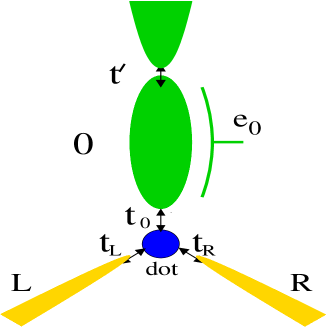
Figure 1: Schematic representation of the device we analyze in this paper. When the box Coulomb blockade energy is not neglected, we assume that the box potential can be controlled by a voltage gate $e_{0}$.

The geometry we analyze is depicted in Fig. 1. In this section we assume that the large dot is connected to a third lead. From hereon, the Coulomb interaction in the box is neglected except in section 5. The Coulomb interaction does not affect the main results we discuss in this section. In order to model the finite-size box connected to a normal reservoir, we choose for convenience a finite-size wire characterized by its length $l$ or equivalently by its level spacing $\Delta\sim\hbar v_{F}/l$. In fact, the precise shape of the finite-size box is not important for our purpose as soon as it is characterized by a mean level spacing $\Delta$ separating peaks in the electronic density of states. We assume that the small quantum dot is weakly coupled to one or two adjacent leads ($L$ and $R$). On the Hamiltonian level, we use the following tight-binding description, and for simplicity model the leads as one-dimensional wires (this is by no means restrictive): $H=H_{L}+H_{R}+H_{0}+H_{dot}+H_{tun}$ with

$$H_{L} = -t\sum_{j=1,s}^{\infty}(c^{\dagger}_{j,s,L}c_{j+1,s,L}+h.c.)-\mu_{L}n_{j,s,L}$$ (1)

$$H_{0} = -t\sum\limits_{j=1,s}^{\infty}(c^{\dagger}_{j,s,0}c_{j+1,s,0}+h.c.)-\mu_{0}n_{j,s,0}$$

$$+(t-t^{\prime})\sum_{s}(c^{\dagger}_{l,s,0}c_{l+1,s,0}+h.c.)$$

$$H_{dot} = \sum_{s}\epsilon_{d}n_{d,s}+Un_{d\uparrow}n_{d\downarrow}$$ (3)

$$H_{tun} = \sum_{s}\sum_{\alpha=L,R,0}(t_{\alpha}c^{\dagger}_{ds}c_{1,s,\alpha}+h.c.).$$ (4)

$H_{R}$ is obtained from $H_{L}$ by changing $L\to R$. Here $c_{j,s,\alpha}$ destroys an electron of spin $s$ at site $j$ in lead $\alpha=0,L,R$; $c_{d,s}$ destroys an electron with spin $s$ in the dot, $n_{j,s,\alpha}=c^{\dagger}_{j,s,\alpha}c_{j,s,\alpha}$ and $n_{ds}=c^{\dagger}_{ds}c_{ds}$. The quantum dot is described by an Anderson impurity model, $\epsilon_{d},U$ are respectively the energy level and the Coulomb repulsion energy in the dot. The tunneling amplitudes between the dot and the left lead, right lead and box are respectively denoted as $t_{L},t_{R},t_{0}$ (see Fig. 1). The tunneling amplitude amplitude between the box and the third lead is denoted as $t^{\prime}$ (see Fig. 1). Finally $t$ denotes the tight binding amplitude for conduction electrons implying that the electronic bandwidth $\Lambda_{0}=4t$. Since we want to use the left and right leads just as transport probes, we assume in the rest of the paper that $t_{L},t_{R}\ll t_{0}$.

We are particularly interested in the Kondo regime where $\langle n_{d}\rangle\sim 1$. In this regime, we can map $H_{tun}+H_{dot}$ to a Kondo Hamiltonian by help of a Schrieffer-Wolff transformation:

$$H_{K}=H_{tun}+H_{dot}=\sum_{\alpha,\beta=L,R,0}J_{\alpha\beta}c_{1,s,\alpha}^{\dagger}\frac{\vec{\sigma}_{ss^{\prime}}}{2}\cdot\vec{S}c_{1,s^{\prime},\beta},$$ (5)

where $J_{\alpha\beta}=2t_{\alpha}t_{\beta}(1/|\varepsilon_{d}|+1/(\varepsilon_{d}+U))$. It is clear that $J_{00}\gg J_{0L},J_{0R}\gg J_{LL},J_{RR},J_{LR}$. In Eq. (5), we have neglected direct potential scattering terms which do not renormalize and can be omitted in the low energy limit.

The Kondo temperature is a crossover scale separating the high temperature perturbative regime from the low temperature one where the impurity is screened. There are many ways to define such scale. We choose the “perturbative scale” which is defined as the scale at which the second order corrections to the Kondo couplings become of the same order of the bare Kondo coupling. Note that all various definitions of Kondo scales differ by a constant multiplicative factor (see for example Ref. simon05 for a comparison between the perturbative Kondo scale with the one coming from the Slave Boson Mean Field Theory).

The renormalization group (RG) equations relate the Kondo couplings defined at scales $\Lambda_{0}$ and $\Lambda$. They simply read:

$$J_{\alpha\beta}(\Lambda)\approx J_{\alpha\beta}(\Lambda_{0})+{1\over 2}\sum_{\gamma}J_{\alpha\gamma}(\Lambda_{0})J_{\gamma\beta}(\Lambda_{0})\left[\int\limits_{\Lambda}^{\Lambda_{0}}+\int\limits_{-\Lambda_{0}}^{-\Lambda}\right]{\rho_{\gamma}(\omega)\over|\omega|}d\omega$$

where $\rho_{\gamma}$ is the LDOS in lead $\gamma$ seen by the quantum dot. Since $J_{00}\gg J_{LL},J_{RR}$, the Kondo temperature essentially depends on the LDOS in the lead $0$. Using the RG equations in Eq. (II), the Kondo temperature can be well approximated as follows:

$${J_{00}\over 2}\left[\int\limits_{T_{K}}^{\Lambda_{0}}+\int\limits_{-\Lambda_{0}}^{-T_{K}}\right]{\rho_{0}(\omega)\over|\omega|}d\omega=1$$ (6)

When the lead $0$ becomes infinite (i.e. when $t^{\prime}=t$), $\rho_{0}(\omega)=\rho_{0}=const$ and we recover $T_{K}=T_{K}^{0}$ the usual Kondo temperature. It is worth noting that including the Coulomb interaction in the box does not affect much the Kondo temperature. The box Coulomb energy $E_{B}$ slightly renormalizes $J_{00}$ in the Schrieffer-Wolff transformation since $E_{G}\ll U,|\epsilon_{d}|$ oreg .

The LDOS $\rho_{0}$ can be easily computed for a finite one-dimensional wire. In general, for a finite size open structure, $\rho_{0}$ corresponds in the limit of a weak coupling to a continuum to a sum of resonance peaks. The positions of these peaks is to a good approximation related to the eigenvalues $\omega_{n}$ of the isolated finite size structure, while their width $\gamma_{n}$ is proportionnal to $t^{\prime 2}|\psi_{n}|^{2}$ where the $\psi_{n}$ are the eigenvectors of the isolated structure. The LDOS $\rho_{0}$ is very well approximated by a sum of Lorentzian functionssimon02 in the limit $t^{\prime}\ll t$ :

$$\pi\rho_{0}(\omega)\approx\sum_{n}|\psi_{n}|^{2}\frac{\gamma_{n}}{(\omega-\omega_{n})^{2}+\gamma_{n}^{2}}.$$ (7)

For a $1D$ finite size wire of length $l$, $\psi_{n}=2\sin(k_{n})/(l+1)$ with $k_{n}\approx\pi n/(l+1)$. This approximation is quite convenient in order to estimate the Kondo temperature $T_{K}$ through (6).

When the level spacing $\Delta_{n}\sim\hbar v_{F}/l$ is much smaller than the Kondo temperature $T_{K}^{0}$, no finite-size effects are expected. Indeed, the integral in (6) averages out over many peaks and the genuine Kondo temperature is $T_{K}\sim T_{K}^{0}$. On the other hand, when $T_{K}^{0}\sim\Delta_{n}$, the Kondo temperature starts to depend on the fine structure of the LDOS $\rho_{0}$ and a careful calculation of the integral in (6) is required. Two cases may be distinguished: either $\rho_{0}$ is tuned such that a resonance $\omega_{n}$ sits at the Fermi energy $E_{F}=0$ (labeled by the index $R$) or in a non resonant situation (labeled by the index $NR$). In the former case, we can estimate

$$T_{K}^{R} = \frac{\gamma_{n}\Delta_{n}}{\sqrt{(\Delta_{n}^{2}+\gamma_{n}^{2})\exp\left(\frac{2}{J_{00}(\Delta_{n})\rho_{0}^{R}(0)}\right)-\Delta_{n}^{2}}}$$ (8)

$$\approx \gamma_{n}\exp\left(-\frac{1}{J_{00}(\Delta_{n})\rho_{0}^{R}(0)}\right)\approx\gamma_{n}\left(\frac{T_{K}^{0}}{\Delta_{n}}\right)^{\frac{\pi\gamma_{n}}{\Delta_{n}}}.$$

In the latter case, we obtain,

$$T_{K}^{NR} = \Delta_{n}\exp\left(-\frac{\pi\Delta_{n}^{2}}{4J_{00}(\Delta_{n})|\psi_{n}|^{2}\gamma_{n}}\right)$$ (9)

$$\approx \Delta_{n}\exp\left(-\frac{1}{J_{00}(\Delta_{n})\rho_{0}^{NR}(0)}\right)\approx\Delta_{n}\left(\frac{T_{K}^{0}}{\Delta_{n}}\right)^{\frac{\pi\Delta_{n}}{8\gamma_{n}}},$$

where $\pi\rho_{0}^{NR}(0)\approx 4\gamma_{n}|\psi_{n}|^{2}/\Delta_{n}^{2}$. These two scales are very different when $t^{\prime 2}\ll t^{2}$. By controlling $\rho_{0}$, we can control the Kondo temperature (at least when $T_{K}\leq\Delta$). The main feature of such geometry is that the screening of the artificial spin impurity is essentially performed in the open finite-size wire corresponding to lead $0$. Now let us study what are the consequences of FSE on transport when one or two leads are weakly coupled to the dot. This is the purpose of the next section.

III Spectroscopy of a Kondo quantum dot coupled to an open box

In this section, we consider a standard three-terminal geometry as depicted in Fig. 1. Since the leads are weakly connected to the dot, they allow a direct access to the dot density of states in presence of FSE in the box.

We have used the Slave Boson Mean Field Theory (SBMFT) hewson in order to calculate the dot local density of states (LDOS). This approximation describes qualitatively well the behavior of the Kondo impurity at low temperature $T\leq T_{K}$ when the impurity is screened and especially capture well the exponential dependence of the Kondo temperature. Furthermore, this method has been proved to be efficient to capture finite size effects in Refs simon02 ; simon05 .

Let us now compute the dot density of states $\rho_{d}(\omega)$. We assuming $\Gamma_{L/R}\ll\Gamma_{0}(\omega)$ such that for low bias the dot Green functions weakly depend on the chemical potential in the left and right leads. Under such conditions, the differential conductance reads as follows:

$$e\frac{dI}{d\mu_{L}}\approx\frac{2e^{2}}{h}4\Gamma_{L}\int\limits_{-\infty}^{\infty}\left(\frac{-df(\omega)}{d\omega}\right)\pi\rho_{d}(\omega+\mu_{L})d\omega.$$ (10)

Varying $\mu_{L}$ allows a direct experimental access to $\rho_{d}(\mu_{L})$ at $T\ll T_{K}$. Note that a similar approximation is used for STM theory with magnetic adatoms schiller00 . We have plotted $\rho_{d}(\omega)$ in Fig. 2 for both the non-resonant case and the on-resonance case for three different values of $\xi_{K}^{0}/l$. We took the following parameters in units of $t=1$: $t_{0}=0.5$, $t_{L}=t_{R}=0.1$ (therefore $t_{L}^{2}<<t_{0}^{2}$), $t^{\prime}=0.5$, and $l\sim 1000a$ ($a$ the lattice constant) or equivalently $\Delta\sim 0.006$. The Kondo energy scale $\xi_{K}^{0}$ can be varied using the dot energy level $\epsilon_{d}$ which is controlled by the dot gate voltage. One has to distinguish between two cases: $T_{K}^{0}\gg\Delta$ and $T_{K}^{0}\ll\Delta$.

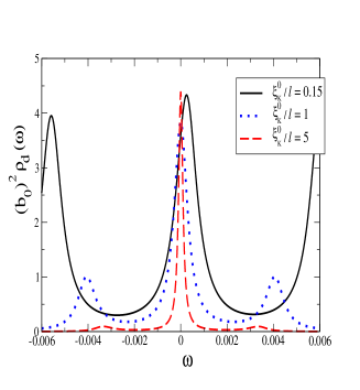
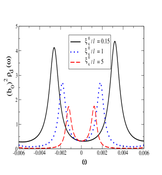
Figure 2: Dot density of states $\rho_{d}(\omega)$ for both the non resonant case (upper panel) and the resonant case (lower panel). We took $\Delta\sim 0.006$ and plot $\rho_{d}$ for $\xi_{K}^{0}/l=\Delta/T_{K}^{0}\sim 0.15$, $\xi_{K}^{0}/l=\Delta/T_{K}^{0}\sim 1$ and $\xi_{K}^{0}/l=\Delta/T_{K}^{0}\sim 5$. Note that $\rho_{d}$ has been scaled by $b_{0}^{2}$, the slave boson parameter for an easy comparison between both cases.

When $T_{K}^{0}\gg\Delta$, no finite-size effect is to be expected. Nevertheless two non trivial features should be be noticed: i) The various peaks appearing in $\rho_{d}$ are included in an envelope of width $O(T_{K}^{0})\gg\Delta$ (which has a broader range than the figure 2 actually covers for $\xi_{K}^{0}/l=\Delta/T_{K}^{0}\sim 0.15$). In this respect, the Kondo resonance plays the role of an energy filtering device which filters the box high energy states that are not in the range of width $O(T_{K}^{0})$ around $E_{F}=0$.

ii) The LDOS $\rho_{d}(\omega)$ mimics the density of state in the lead $0$ but is shifted such that an off-resonance peak in the lead $0$ corresponds to a dot resonance peak and vice versa. This can be simply understood from a non-interacting picture valid at $T=0$. The non-interacting dot Green function reads

$$G_{dd}(\omega)\approx\frac{1}{\omega-\epsilon_{d}-\delta\epsilon(\omega)+i\Gamma_{0}(\omega)},$$ (11)

where $\delta\epsilon$ is the real part of the dot self-energy and $\Gamma_{0}$ its imaginary part. The minima’s of $\Gamma_{0}$ thus correspond to the maxima of $-Im(G_{dd})$. We also note that the resonance peak is slightly shifted from $\omega=0$ in this limit. Therefore the 2-terminal conductance does not reach its unitary limit (i.e. its maximum non interacting value). This is due to the fact that we took $\epsilon_{d}=-0.68$ and we are not deep in the Kondo regime. Particle-hole symmetry is not completely restored in the low energy limit.

On the other hand, when $\xi_{K}^{0}\gg l$ ($T_{K}^{0}\ll\Delta$), $\rho_{d}$ changes drastically. The fine structure in the box density of states no longer shows up in $\rho_{d}$. This is expected since only the energy states which are within a range of order $O(T_{K})\ll\Delta$ appears in the dot LDOS. In the off-resonance case, only the narrow Kondo peak of width $T_{K}^{NR}\ll T_{K}^{0}$ mainly subsists for $\xi_{K}^{0}/l=5$ (upper panel of Fig. 2). We can also show that the position of the small peaks at $\omega\sim\pm\Delta/2$ for $\xi_{K}^{0}\gg l$ are related to the resonance peaks in lead $0$. We also note that the narrow peak is this time almost at $\omega=E_{F}=0$ i.e. particle-hole symmetry is restored. In order to reach large value of $\xi_{K}^{0}$, we took small values of $\epsilon_{d}$ such that we are deep in the Kondo regime where $n_{D}\sim 1$.

The most surprising result occurs for the resonant case where the Kondo peak is split for $\xi_{K}^{0}\gg l$. Usually a splitting of the Kondo LDOS is associated with the destruction of the Kondo effect as this would be the case for a Kondo quantum dot under a magnetic field or interacting with another quantum dot via the RKKY interaction craig ; rkky ; vavilov . Here the splitting cannot at all be attributed to the destruction of the Kondo effect but instead to a subtle non interacting destructive interference phenomenon. Let us use some renormalization group argument. When we integrate out high energy electronic degrees of freedom from the bandwidth down to an energy scale of order $\Delta>T_{K}^{0}$, we start building the Kondo resonance at the Fermi energy $E_{F}$. If we continue integrating out electronic degrees of freedom from $\Delta$ down to $\gamma$, this reasoning would tell us that we end up with a Kondo resonance pinned at $E_{F}$. However, this does not take into account that the box has also a (non interacting) resonance pinned at $E_{F}$ and these two resonances are coupled via the tunnel amplitude $t_{0}$. By analogy to a molecular system with two degenerate orbital states, where a tunneling amplitude leaves the degeneracy and creates bonding and anti-bonding states, a strong $t_{0}$ (as is our case here) may lead to a splitting of the Kondo resonance. Therefore this splitting is more related to a destructive interference between the two resonances -an interacting one in the dot and a non-interacting one in the box. The study of the splitting of the Kondo resonance as a function of $t_{0}$ has been extensively studied recently in a slightly different geometry by Dias da Silva et al. sandler . One can also quantify this splitting within the SBMFT method. By approximating $\Gamma_{0}(\omega)\approx t_{0}^{2}|\psi_{n}|^{2}\frac{\gamma_{n}}{\omega^{2}+\gamma_{n}^{2}}$ at a resonance $n$, one can well understand analytically the structure of $\rho_{d}$. When $T_{K}^{R}\gg\gamma_{n}$, one can show that the peak splitting is of order $\sim 2\sqrt{\gamma_{n}T_{K}^{R}}$ and the peaks width is of order $\gamma_{n}$.

IV Analysis of transport properties

At $T=0$, it is straightforward to show, using for example the scattering formalism,ng that the conductance matrix $G_{\alpha,\beta}^{U}$ is simply given by

$$G_{\alpha,\beta}^{U}=\frac{2e^{2}}{h}{4\Gamma_{\alpha}\Gamma_{\beta}\over(\Gamma_{L}+\Gamma_{0}+\Gamma_{R})^{2}}$$ (12)

where $\Gamma_{\alpha}=\pi t_{\alpha}^{2}\rho_{\alpha}(0)$, and $\alpha=l,0,r$. Since the SBMFT aims at replacing the initial Anderson Hamiltonian by a non-interacting one, one may easily access the conductance by directly applying the Landauer formula or equivalently by using

$$G_{\alpha\beta}=\frac{2e^{2}}{h}\int d\omega\left(\frac{-\partial f}{\partial\omega}\right){4\Gamma_{\alpha}(\omega)\Gamma_{\beta}(\omega)\over(\sum_{\alpha}\Gamma_{\alpha}(\omega))}Im(-G_{dd}^{r})(\omega).$$ (13)

Using the SBMFT, one can extensively study the conductance as function of temperature for various case $T_{K}^{0}\gg\Delta$, $T_{K}^{0}\ll D$. This has been reported in details in julien . Actually, it turns out that finite size effects, which are related to the finite size extension of the Kondo cloud, are clearly visible at some intermediate temperature $T_{K}^{0}>T>T_{K}^{R},T_{K}^{NR}$. In this temperature range, significant deviations from the non-interacting limit are obtained. Let us assume that the box can be gated (see Fig. 1). We took the same parameters as in Fig. 2 except that $l=200a$. The finite size effects are much more spectacular when one look at the conductance, at fixed temperature, as a function of the box gate voltage $e_{0}$. We have therefore fixed the temperature at $T=2.10^{-3}$ and plotted the conductance $G_{L0}$ as a function of $e_{0}$ for different values of $\xi_{K}$, controlled here by the parameter $\epsilon_{d}$. The other parameters are unchanged. The upper (plain style) curve corresponds to $\xi_{K}=50a<l$. We observe large oscillations of the conductance corresponding to $e_{0}$ being on a resonance or off a resonance. At large $\xi_{K}\sim 1000a\gg l$, the conductance (dashed-dashed-dotted style) has a completely different shape. The minima’s and the maxima’s of the conductance at $\xi_{K}\sim 50a$ become now respectively maxima’s and minima’s. Furthermore the conductance at these minima’s is very small close to $0$. This regime corresponds to the high temperature for the non resonant case. The intermediate values of $\xi_{K}$ show how the conductance crosses over in between these two extreme cases. This dramatic change of the conductance in the regime in which $\xi_{K}\gg l$ is a direct consequence of interactions effects and should be directly observable in experiments. Similar results can be obviously obtained by analyzing the conductance $G_{LR}$ despite the fact that the amplitude of $G_{LR}$ will be in general smaller than $G_{L0}$ by a factor $\sim\sqrt{\Gamma_{L}\Gamma_{R}}/\Gamma_{0}$. In fact, the conductance $G_{LR}$ can be made significantly larger by adjusting the chemical potential $\mu_{0}$ such that the current in lead $0$ verifies $\langle I_{0}\rangle=0$.

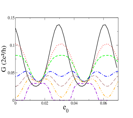
Figure 3: Conductance (in units of $2e^{2}/h$) as a function of $\varepsilon_{W}$ for different values of $\xi_{K}$. From top to bottom $\xi_{K}\sim 50a$ (plain style), $\xi_{k}\sim 150a$ (dotted style), $\xi_{K}\sim 300a$ (short dashed style), $\xi_{K}\sim 500a$ (dot-long dashed style), $\xi_{K}\sim 600a$ (long dashed style), $\xi_{K}\sim 750a$ (dot-dot-dashed style) and $\xi_{K}\sim 1000a$ (dot-dashed-dashed style)

We have essentially used the SBMFT to analyze the spectroscopic and transport properties. Nevertheless, one can also use analytical calculations in two limiting cases. When $T\gg T_{K}$, one can safely rely on renormalized perturbative calculations while at $T\ll T_{K}$ the Nozières Fermi liquid approach nozieres can be applied. Using the latter theory, one can for example show that the conductance in the on resonance case is a non monotonous function of temperature. We refer the reader to Ref. julien where these analytical calculations are detailed and confirm the present analysis.

V Finite box Coulomb energy

In this section, we discuss whether a finite box Coulomb energy modifies or not the results presented in this work. As we already mentioned in section 2, the Kondo coupling $J_{00}$, is almost not affected by the box Coulomb energy $E_{B}$ (since $E_{B}\ll U$) and therefore the Kondo temperature remains almost unchanged. As shown in oreg ; borda04 ; florens , a small energy scale $E_{B}$ changes the renormalization group equation in Eq. (II). The off-diagonal couplings $J_{0L}(\Lambda),J_{0R}(\Lambda)$ tend to $0$ for $\Lambda\ll E_{B}$. At energy $\Lambda\ll E_{B}$ the problem therefore reduces to an anisotropic $2-$channel Kondo problem. The strongly coupled channel is the box $0$, the weakly coupled one is the even combination of the conduction electron in the left/right leads. At very low energy, the fixed point of the anisotropic $2-$channel Kondo model is a Fermi liquid. It is characterized by the strongly coupled lead (here the box) screening the impurity whereas the weakly coupled one completely decoupled from the impurity. The dot density of states depicted in Fig. 2 should remain therefore almost unaffected. The problem is to read the dot LDOS with the weakly coupled leads since they decouple at $T=0$. Nevertheless, for a typical experiment done at low temperature $T$, such a decoupling is not complete and the dot LDOS should be still accessible using the weakly coupled leads but with a very small amplitude.

We up to now analyze the situation in which a box or a finite size wire is also used as a third terminal i.e is coupled to a continuum. In some situations, like the theoretical one presented in Ref. oreg , no terminal lead is attached to the box and the geometry is a genuine 2-terminal one. In order to analyze this system, we have to take into account both a finite level spacing and a finite box Coulomb energy. One can make progress if we assume $T_{K0}\ll\Delta\ll E_{B}\ll U\ll D_{0}$ where $D_{0}$ is the bandwidth. One proceeds with a RG treatment in three steps: $E_{B}<<\Lambda<<U$, $\Delta<<\Lambda<<E_{B}$ et $T_{K0}<<\Lambda<<\Delta$. When $E_{B}<<\Lambda<<U$, the RG equations derived in Eq. (II) remain valid and are the usual ones. When $\Delta<<\Lambda<<E_{B}$, the couplings $J_{L0}$ and $J_{R0}$ stop renormalizing because of the Coulomb energy $E_{B}$. The other couplings keep on growing. When $T_{K0}<<\Lambda<<\Delta$, two situations are to be considered. Let us start with the case where no resonance sits at the Fermi energy in the box. The coupling $J_{00}$ no longer renormalizes since there is no state available. On the other hand, the couplings $J_{\alpha,\beta}$ with $\alpha,\beta=L,R$ keep on renormalizing and may eventually reach a strong coupling regime. Therefore, the screening of the impurity ultimately occurs in the $L,R$ leads though we may have started with $J_{00}\gg J_{LL},J_{RR}$. This situation is quite different than the one we explored previously. However, when a resonance sits at the Fermi energy of the box, we are left with a double dot problem with one electron in each dots. They form a singlet and we expect a split LDOS in the dot. If we assume $E_{B}\ll\Delta$, the problem gets more complicated since we already reach a strong coupling regime at the scale $E_{B}$. A step toward this direction was recently achieved in Ref. kaul06 in a slightly modified geometry.

VI Conclusions

In this paper, we have studied a geometry in which a small quantum dot in the Kondo regime is strongly coupled to a large open quantum dot or open finite size wire and weakly coupled to other normal leads which are simply used as transport probes. The artificial impurity is mainly screened is the large quantum dot. Such a geometry thus allows to probe the dot spectroscopic properties without perturbing it. We have shown using the SBMFT how finite size effects show up in the dot density of states and in the the conductance matrix. We also analyzed how these results are modified in presence of Coulomb interactions in the box. We hope the predictions presented here are robust enough to be checked experimentally.

Acknowledgements This research was partly supported by the contract PNANO ‘QuSpins’ of the French Agence Nationale de la Recherche.

References

- (1) A. C. Hewson, The Kondo Problem to Heavy Fermions, (Cambridge University Press, Cambridge, UK, 1997).
- (2) D. Goldhaber-Gordon, H. Shtrikman, D. Mahalu, D. Abusch-Magder, U. Meirav, and M. A. Kaster, Nature 391, 156 (1998).
- (3) S. M. Cronenwett, T. H. Oosterkamp, and L. P. Kouwenhoven, Science 281, 540 (1998).
- (4) F. Simmel, R. H. Blick, U.P. Kotthaus, W. Wegsheider, and M. Blichler, Phys. Rev. Lett. 83, 804 (1999).
- (5) W. G. van der Wiel, S. De Franceschi, T. Fujisawa, J. M. Elzerman, S. Tarucha, and L. P. Kouwenhoven, Science, 289, 2105 (2000).
- (6) J. Nygård et al., Nature 408, 342 (2000).
- (7) M. R. Buitelaar et al., Phys. Rev. Lett. 88, 156801 (2002).
- (8) P. Jarillo-Herrero et al., Nature 434, 484 (2005).
- (9) J. Park et al., Nature 417, 722 (2002); W. Liang et al., Nature 417, 725 (2002).
- (10) W. B. Thimm, J. Kroha, J. von Delft, Phys. Rev. Lett. 82 2143 (1999).
- (11) T. Hand, J. Kroha, and H. Monien, Phys. Rev. Lett. 97, 136604 (2006).
- (12) I. Affleck and P. Simon, Phys. Rev. Lett. 86, 2854 (2001); P. Simon and I. Affleck, Phys. Rev. B 64, 085308 (2001).
- (13) H. Hu, G.-M. Zhang, and Yu Lu, Phys. Rev. Lett. 86, 5558 (2001).
- (14) E. S. Sorensen, I. Affleck, Phys. Rev. Lett. 94, 086601 (2005).
- (15) P. Simon, O. Entin-Wohlmann, and A. Aharony, Phys. Rev. B 72, 245313 (2005).
- (16) P. Simon and I. Affleck, Phys. Rev. B 68, 115304 (2003); P. Simon and I. Affleck, Phys. Rev. Lett. 89 206602 (2002).
- (17) P. S. Cornaglia and C. A. Balseiro, Phys. Rev. Lett. 90, 216801 (2003).
- (18) P. Simon, Phys. Rev. B 71, 155319 (2005).
- (19) Note that for a or metallic box, the level spacing is not simply related to the Fermi velocity and the length scale of the box. In this case, we shall compare directly to .
- (20) Y. Oreg and D. Goldhaber-Gordon, Phys. Rev. Lett. 90, 136602 (2003).
- (21) N. J. Craig, J. M. Taylor, E. A. Lester, C. M. Marcus, M. P. Hanson, and A. C. Gossard, Science 304, 565 (2004).
- (22) A. Schiller and S. Herschfield, Phys. Rev. B 61, 9036 (2000).
- (23) P. Simon, R. Lopez, and Y. Oreg, Phys. Rev. Lett. 94, 086602 (2005).
- (24) M. Vavilov and L. Glazman ibid. 94, 086805 (2005).
- (25) L. G. G. V. Dias da Silva, N. Sandler, K. Ingersent, and S. Ulloa, Phys. Rev. Lett. 97, 096603 (2006).
- (26) T. K. Ng and P. A. Lee, Phys. Rev. Lett. 61 1768 (1988).
- (27) P. Simon, J. Salomez, and D. Feinberg, Phys. Rev. B 73, 205325 (2006).
- (28) P. Nozi\a‘eres, J. Low Temp. Phys. 17 31 (1974).
- (29) M. Pustilnik, L. Borda, L. I. Glazman, and J. von Delft, Phys. Rev. B 69, 115316 (2004).
- (30) S. Florens and A. Rosch, Phys. Rev. Lett. 92, 216601 (2004).
- (31) R. K. Kaul, G. Zarand, S. Chandrasekharan, D. Ullmo, and H. U. Baranger, Phys. Rev. Lett. 96, 176802 (2006)