Evolution of supermassive black holes

Abstract

The cosmological evolution of supermassive black holes (SMBHs) seems to be intimately linked to their host galaxies. Active galactic nuclei (AGN) can be probed by deep X–ray surveys. We review results from large X–ray selected samples including first results from the XMM–Newton COSMOS survey. A new picture arises from the fact that high–luminosity AGN grow earlier than low–luminosity AGN. In particular, the space density of low–luminosity AGN exhibits a significant decline for redshifts above z=1. This ”anti–hierarchical” growth scenario of SMBHs can be explained by two modes of accretion with different efficiency. The population of Compton–thick sources plays a key role in our understanding of the BH growth history. Their space density and redshift distribution is relevant to estimate the SMBH mass function. A comparison with the relic SMBH mass distribution in the local Universe constrains the average radiative efficiency and Eddington ratio of the accretion. We discuss a new synthesis model of Compton–thin and Compton–thick sources that is in concordance with deep X–ray observations and in particular predicts the right level of contribution of the Compton–thick source population observed in the Chandra Deep Field South observations as well as the first INTEGRAL and Swift catalogues of AGN. Currently, one of the most important problems is the evolution of obscuration with redshift.

1 Introduction

1.1 Deep surveys

Deep field observations are a suitable observational technique to probe AGN physics. In multi–wavelength campaigns, astronomers select a field in the sky and produce images from several pointings. They use a combination of wide fields to collect many sources and so–called pencil beams to investigate sources in deep space. Today, there are many samples in different wavelength bands available and large surveys are underway. Among the most important deep extragalactic surveys to date are the two fields related with the GOODS survey, the Hubble Deep Field North (HDF N) and the Chandra Deep Field South (CDF–S), the latter field encompassing the Hubble Space Telescope ACS Ultradeep Field (HUDF) and embedded in the larger GEMS, COMBO-17 and ECDFS surveys. The COSMOS project is a multiwavelength survey centered around the largest HST observing project, covering 2 square degrees.

On the basis of multi–wavelength observations and in comparison with galaxy and accretion models it turns out that AGN are mainly determined by the following physical parameters: accretion rate, accretion efficiency, SMBH mass, SMBH spin, stellar formation rate, metallicity, dusty torus mass, and seed magnetic field. One geometric parameter is the inclination angle of the system. The challenge consists in determining these parameters from observations and to fit them into an AGN unification model.

The innermost part of AGN can be probed by means of X–ray observations. The hot inner accretion flows produce soft and hard X–rays. Hence, X–ray deep surveys provide an important issue to study AGN and their SMBHs inside.

Thereby, astronomers are confronted with observational challenges as well. In X–ray deep surveys the redshift of the sources is optically determined by using spectroscopic techniques (spectro–z) or by photometric techniques (photo–z). At high cosmological redshifts the I band magnitudes are faint and in certain redshift ranges spectroscopic features are weak or absent, therefore astronomers fail to determine spectro–z’s. The problem of spectroscopic incompleteness emerges typically at $1<z<2$ – a phenomenon that was coined ’spectroscopic desert’ (see e.g. [Brandt & Hasinger 2005]).

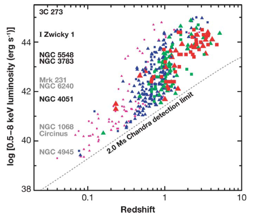
Figure 1: Rest–frame 0.5-8 keV luminosity as function of redshift for sources form the CDF–N (triangles) and CDF–S (squares). The data points are grouped above the 2 Ms Chandra detection limit (dotted line). The ’spectroscopic desert’ is visible on the right–hand side in the luminosity–redshift plane (taken from [Brandt & Hasinger 2005]).

Figure 1 illustrates the sources in the luminosity–redshift plane. The I band magnitudes successively grow from left to right until the emission drops below the spectroscopic sensitivity limit of 8–10 m class telescopes, leaving a lack of spectroscopically identified sources on the on the right–hand side of the plot close to the sensitivity limit. In the CDF–S it is possible to fill this spectroscopic desert with photo–z thanks to a combination of the deep multiwavelength photometry available through GOODS, GEMS and COMBO-17 in this field ([Szokoly et al. 2004, Zheng et al. 2004, Mainieri et al. 2005, Wolf et al. 2004, Grazian et al. 2006]). As a result, it is possible to obtain 95% redshift completeness for the CDF–S. Redshift completeness of X–ray flux limited samples is vital to produce statistically and systematically reliable results. Therefore in the further analysis we typically cut all samples to a $>80\%$ redshift completeness, leading to an overall completeness of the sample of $\sim 90\%$.

1.2 AGN classification criteria

The classical discrimination between type–1 (unobscured) and type–2 (obscured) AGN is done using a classification through optical spectroscopy. Optical type-1 AGN have broad permitted emission lines, while optical type–2 AGN do not show broad permitted lines, but still have high-excitation narrow emission lines. Therefore, many works in the field are mainly using the presence of broad lines as discriminator and classify type-1 AGN only as Broad-line AGN (BLAGN). However, this AGN classification scheme breaks down, when the optical spectrum is insufficient to discriminate the line widths. At high redshifts and low luminosities there are several effects that compromise the optical classification. First, in general high redshift objects are faint, so that they require very long observing times to obtain spectra of sufficient quality and unambiguously discern broad emission line components. Secondly, there are redshift ranges, where the classical broad lines shift out of the observed optical bands (see above). Thirdly, and probably most importantly, at high redshifts the spectroscopic slit is filled with the whole light of the AGN nucleus and the host galaxy. Depending on the ratio between nuclear and host luminosity, the host galaxy can easily outshine the AGN nucleus, rendering the AGN invisible in the optical light. This is the main reason, why X–ray samples are much more efficient in picking up low-luminosity AGN at high redshift.

In principle, a classification purely based on X–ray properties would be possible. Large hydrogen column densities block soft X–rays. Therefore, a suitable AGN classification scheme in X–rays could involve the column density $N_{\rm H}$ that can be determined from the X–ray spectra. Usually, AGN X–ray spectra are fit by simple power law models. The effect of increasing column density is that the soft part of the spectrum is more and more suppressed, i.e. the spectrum becomes harder at high $N_{\rm H}$. Correlations between optical and X–ray properties of obscured and unobscured AGN show a very good match ($\sim 90\%$) between optical obscuration and X–ray absorption. It is therefore suitable to define an X–ray type–1 AGN by $\log N_{\rm H}<22$ whereas AGN type–2 satisfy $\log N_{\rm H}>22$. However, in practice is not possible to determine $N_{\rm H}$ values for samples with typically very faint X–ray sources, due to the small number of observed photons. Therefore, one has to resort to hardness ratios measured from coarse X–ray bands. The determination of $N_{\rm H}$ values from X–ray hardness ratios, in particular at high redshifts is biased towards too high absorption values (see e.g. [Tozzi et al. 2006]), so that the X–ray classification alone also introduces significant systematic errors.

To overcome the difficulties of classification in either the optical or the X–ray bands, a combined optical/X–ray classification scheme has been introduced ([Szokoly et al. 2004, Zheng et al. 2004]). It involves a threshold X–ray luminosity $L_{\rm X}$ and the X–ray hardness ratio HR, defined as

$${\rm HR}=({\rm H}-{\rm S})/({\rm H}+{\rm S}),$$ (1)

with count rate in the hard band H and soft band S. The threshold AGN X–ray luminosity is set at for an AGN $\log L_{\rm X}>42$, roughly at the upper luminosity range of vigorously star forming galaxies. The practical combined optical/X–ray AGN classification is the following: An optical broad–line AGN (BLAGN) or a galaxy with $\log L_{\rm X}>42$ and hardness ratio ${\rm HR}<-0.2$ is called an AGN type–1. An optical narrow-line AGN (NLAGN) or a galaxy with $\log L_{\rm X}>42$ and hardness ratio ${\rm HR}>-0.2$ is called an AGN type–2.

This classification has the advantage that it can also be applied for sources, which have only photometric redshifts and no spectroscopic information at all. The other advantage is, that it is based on a simple measurable quantity, the hardness ratio. There are also obvious systematic effects and difficulties. A small fraction of AGN are known not to follow the simple optical/X–ray obscuration/absorption correlation, either broad line AGN have absorbed X–ray spectra (e.g. for BAL QSOs), or narrow-line AGN have unabsorbed X–ray spectra (e.g. for narrow-line Seyfert-1 galaxies or Compton-thick, reflection dominated spectra). Also the hardness ratio threshold is a function of redshift. Finally, the dust obscuration versus gas absorption properties may be different, depending on environment and redshift. Nevertheless, we consider these systematic effects far smaller than those of any of the other classifications individually. All the systematics addressed here can in principle be quantified through appropriate theoretical population synthesis models.

2 Separate evolution of AGN classes

2.1 Anti–hierarchical growth of SMBHs

Deep surveys supply the X–ray luminosity functions (XLF) and bolometric luminosity functions of AGN. Using soft X–ray luminosity functions, Hasinger et al.(2005) could confirm that the density evolution depends significantly on AGN luminosity, i.e. the cosmological evolution of high–luminosity AGN (HLAGN) deviates strongly from that of low–luminosity AGN (LLAGN): the space density of HLAGN peaks at higher redshift $z\sim 2$ but the space density of LLAGN peaks at $z\sim 0.7$. This systematic trend of active SMBHs has been coined ’anti–hierarchical growth’ or ’cosmic downsizing’. It is possible to understand this behaviour in the framework of accretion theory ([Merloni 2004]). The observed local black hole mass function (BHMF) is taken as boundary condition to integrate the continuity equation backwards in time (mergers are neglected). It could be shown that the most massive SMBH with billions of solar masses were already in place at $z\simeq 3$. Indeed, this is observed for some SDSS quasars [(Fan et al. 2003)]. Merloni (2004) has also demonstrated that radiatively inefficient accretion (e.g. ADAF solutions) dominate only at $z<1$. Therefore, Seyfert galaxies and quasars evolve cosmologically in a radically different manner. The bulk of AGN has to wait much longer to grow or to be activated.

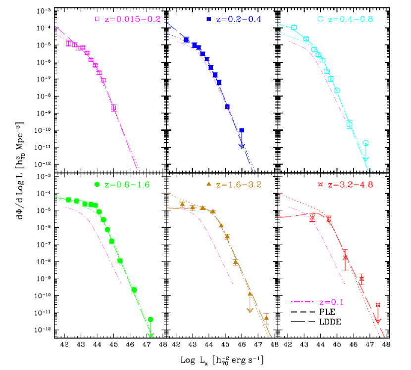
Figure 2: Observed 0.5-2 keV luminosity functions for AGN type–1 in six different redshift ranges. The solid curves through the data points are best luminosity–dependent density evolution (LDDE) fits. For comparison, the curve from the upper left panel ($z=0.015-0.2$) is plotted in all other panels. Adapted from [Hasinger et al. 2005].

The soft X–ray (0.5-2 keV) luminosity functions for AGN type–1 in six different redshift ranges are shown in figure 2. Here, a successive evolution along redshift is visible. Only a luminosity–dependent density evolution (LDDE) can describe the data. Pure luminosity evolution (PLE) or pure density evolution (PDE) models are inadequate.

Now, there is firm evidence of a decline in space density of LLAGN towards higher redshift. For HLAGN, i.e. high–mass BHs deep X–ray surveys so far provide rather poor constraints about their growth phase in the redshift range $3\lesssim z\lesssim 6$ ([Hasinger et al. 2005, Silverman et al. 2005]), while in the optical and radio bands a clear decline of space density is observed for $z>3$ ([Fan et al. 2001, Wall et al. 2005]).

The observed luminosity functions have also been compared to other models. [Marconi et al. 2004] compared the mass function of black holes (BHs) in the local universe with that from AGN relics. The basic idea is that the relic BHs are grown from seed BHs by accretion in AGN phases. The local black hole mass function (BHMF) is estimated by using the prominent correlations between BH mass, stellar velocity dispersion and bulge luminosity. Again, merging is neglected in this model. Then, it is possible to derive the average radiative efficiency $\epsilon$ and the ratio between emitted and Eddington luminosity $\lambda=L/L_{\rm Edd}$ and the average lifetime of active BHs. Based on this model, typical efficiencies are found to be $\epsilon=0.04-0.16$ and Eddington luminosities $\lambda=0.1-1.7$. The BH lifetime strongly depends on BH mass and amounts to 450 million years for 100 solar mass BHs and 150 million years for most massive BHs with more than billion solar masses.

The luminosity functions from SDSS ([Richards et al. 2006]), from hard X–rays ([La Franca et al. 2005]) and soft X–rays (Hasinger et al. 2005) are fairly consistent with the model by Marconi et al.(2004). Soltan’s original argument ([Soltan 1982]) can be extended: one compares the accreted BHMF derived from the cosmic X–ray background with the MF of dormant relic BHs in local galaxies. Both can be reconciled if an energy conversion efficiency of $\epsilon=0.1$ is assumed. From accretion theory it is known that such high efficiencies involve a Kerr BH, i.e. active BHs in AGN have to rotate. Other work on cosmological BH growth also indicates high BH spins ([Volonteri et al. 2005]).

Recently, bolometric quasar luminosity functions have been determined and they agree well with the X–ray data in each redshift slice. They demonstrate a perfect match between the soft X–ray, hard X–ray, optical and even MIR wavebands, when the appropriate bolometric corrections and absorption distributions are taken into account [(Hopkins et al. 2007)]. Because the optical and soft X–ray luminosity functions refer to type-1 AGN only, while the hard X–ray and MIR luminosity functions refer to all AGN, this agreement gives a kind of sanity-check on the type–1/type–2 classification discussed above. [Barger et al. 2005], using a pure BLAGN classification, on the contrary find a strong decline of the type–1 space density at the low–luminosity end.

Recent multi–scale simulations have shown that it is possible to explain the highest redshift, massive SDSS quasar SMBHs by gas accretion plus major mergers in a small group of protogalaxies within the framework of standard $\Lambda$CDM cosmology ([Li et al. 2006]). This picture immediately calls for deeper observations because the known quasars with billion solar masses SMBHs at $z\simeq 6$ should possess progenitors, i.e. the so–called mini-quasars with million solar masses at $z\simeq 10$ and stellar BHs with a few hundred solar masses at $z\simeq 20$. It is the task of future X–ray missions to probe these progenitors.

2.2 Luminosity–dependence of AGN type–2 fraction

A grouping into luminosity classes is one issue to prove the separate evolution of AGN classes. Here we summarize recent work on the AGN type–2 fraction. [Ueda et al. 2003] studied the hard X–ray luminosity functions of an ASCA sample with $\sim$230 sources which was highly complete, $\sim 95$%. They found that the fraction of type–2 AGN decreases with X–ray luminosity, $L_{\rm 2-10\,keV}$. Similar results have been obtained with different systematics by the CLASXS team ([Steffen et al. 2003]) and by Hasinger (2004). Our preliminary analysis ([Hasinger 2007]) confirms this trend in much more detail and better statistics using different data sets from XMM–Newton, Chandra, ASCA and HEAO-1 (see figure 3). Further, [OIII]–selected Seyfert galaxies of the SDSS agree with this trend [(Simpson 2005)]. It has been demonstrated in this work that for Seyfert galaxies selected in the SDSS, the fraction of BLAGN increases with the luminosity of the isotropically emitted [O III] narrow emission line. The [O III] luminosity can be converted into a 2-10 keV luminosity by empirical relations found for Seyfert galaxies [(Mulchaey et al. 1994)], i.e. $L_{{\rm[OIII]}}=0.015\,L_{\rm 2-10\,keV}$.

Figure 3 illustrates all this work in direct comparison.

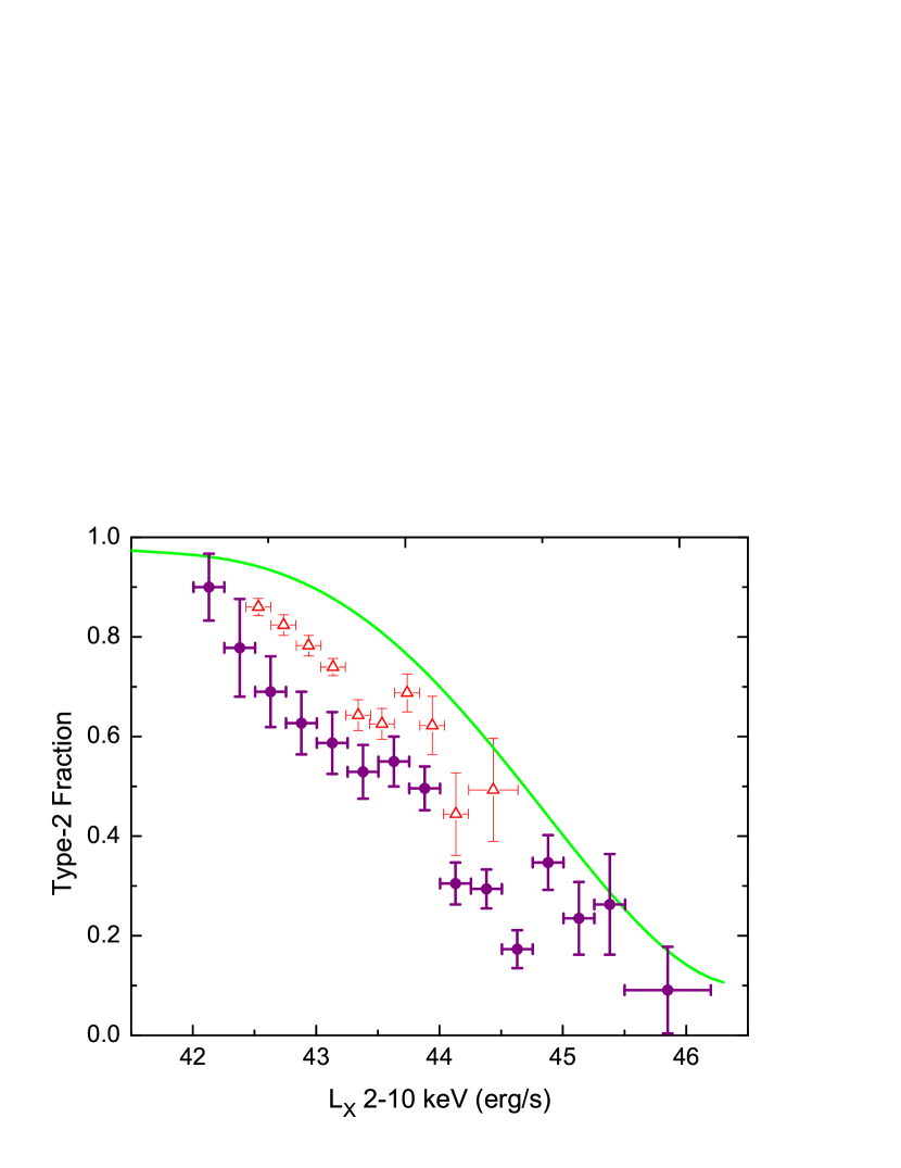
Figure 3: The luminosity dependence of the type–2 fraction compiled from different work. The X–ray data (filled circles) are from a sample of 1029 AGN selected in the 2-10 keV band, with $>90\%$ redshift completeness ([Hasinger 2007]). The triangles are from a sample of [OIII] selected AGN from the SDSS [(Simpson 2005)]. The solid line is from silicate dust studies of a sample of AGN observed with Spitzer in the MIR ([Maiolino et al. 2007]). Given the known selection effects in the different bands, the data are consistent with each other and exhibit the same trend of decreasing absorption with luminosity.

Of course, both the X–ray and optical wavelength bands are subject to selection effects and biases: X–rays in the 2–10 keV band miss the population of Compton–thick Seyferts; optical surveys miss the AGN population diluted by the host galaxy. Nevertheless, the agreement of better than 20% between the optical and X–ray selection is reassuring. Physically, this luminosity–dependent fraction might be interpreted as a ’cleanout effect’ because more luminous AGN can dissociate, ionize and finally blow away the dust in their environment. Recently, mid–infrared (MIR) Spitzer observations of 25 luminous and distant quasars additionally confirm this picture ([Maiolino et al. 2007]). They find a non–linear correlation between 6.7$\mu$m MIR emission and 5100 Å optical emission. This is interpreted as decreasing covering factor of circumnuclear dust as function of luminosity. Further, the silicate emission strength correlates with the luminosity, the accretion rate $L/L_{\rm Edd}$ and black hole mass $M_{\rm BH}$.

The evolution of this luminosity–dependent obscuration fraction with redshift is still a matter of intense debate. A redshift depencence of the obscured fraction was claimed by [Fiore et al. 2003], using the HELLAS2XMM sample. On the other hand, other authors ([Ueda et al. 2003, Gilli et al. 2007]) did not find a redshift dependence. Recently, Treister and Urry (2006) performed a similar analysis, using an AGN meta–sample of 2300 AGN with $\sim 50\%$ redshift completeness and find a shallow increase of the type–2 AGN fraction proportional to $(1+z)^{0.3}$. The differences between the various results could be due to the way the redshift incompleteness, the different flux limits and the AGN classification have been taken into account in the analysis.

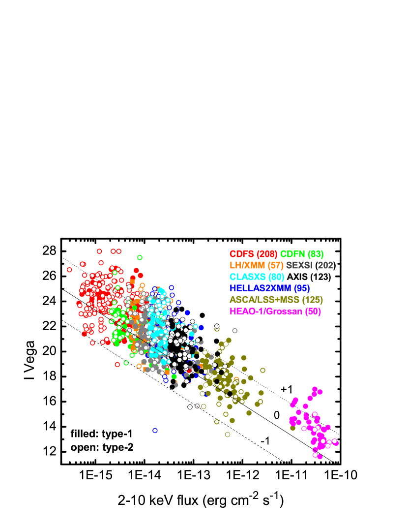
Figure 4: Hard X–ray (2–10 keV) sample of 1029 AGN in the I–flux plane. The individual samples have been cut a flux limit yielding $>80\%$ redshift completeness: CDF–S ([Szokoly et al. 2004, Zheng et al. 2004, Grazian et al. 2006]), CDF–N ([Barger et al. 2003]), LH/XMM ([Mainieri et al. 2002, Szokoly et al. 2007]), SEXSI ([Eckart et al. 2006]), CLASXS ([Steffen et al. 2004]), AXIS ([Barcons et al. 2007]), HELLAS2XMM ([Fiore et al. 2003]), ASCA LSS & MSS ([Akiyama et al. 2000, Ueda et al. 2005]), HEAO-1 / Grossan ([Shinozaki et al. 2006])

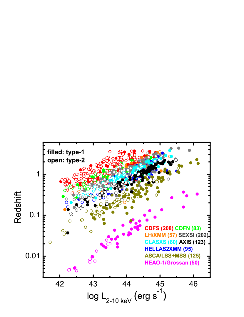
Figure 5: The same sample as figure 4 in the redshift–luminosity plane.

Here, we shortly report on ongoing work ([Hasinger 2007]) on a sample of $\sim$1000 AGN selected in the 2–10 keV band with $\sim$90% optical redshift completeness. In figure 4 and 5 we show the 2-10 keV AGN samples utilized in this analysis in an X–ray flux/optical magnitude and an X–ray luminosity/redshift diagram. Type–1 and type–2 AGN of the different samples are shown with filled and open circles, respectively. Just looking at the data, there is a noticable change of the fraction of type–2 AGN as a function of luminosity. This trend becomes very obvious, if the data is integrated in the redshift range z=0.2–3.2 and the type–2 fraction is displayed as a function of X–ray luminosity (figure 3.)

In order to address a possible evolution of the obscuration fraction with redshift, one can first simply determine the observed ratio of type–2 versus total AGN, integrated over all luminosities, in shells of increasing redshift. This is very similar to what was done by Treister & Urry (2006). Figure 6 shows the observed change of the observed fraction of absorbed objects with redshift. Despite the rather different selection effect and redshift incompleteness (90% vs. 50%), the observed data of Hasinger (2007) and Treister & Urry (2006) agree very well at redshifts above $z=1.5$. At lower redshifts the Treister & Urry values are systematically above those of Hasinger, which is probably due to the fact, that the former authors have only included BLAGN in their type-1 selection and thus systematically overpredict the number of obscured sources.

The diagram also shows an attempt to estimate the possible effects of the small but still significant redshift incompleteness in the sample. For each redshift shell all the unidentified sources were placed at the center of the corresponding shell and included in the type–1 or type–2 classification, depending on their measured hardness ratios and assumed luminosities. This is clearly a very conservative limit, since it is highly unlikely that all the missing redshifts fall into one bin. Finally, the diagram also shows the type–2 fraction as a function of redshift predicted from the most recent background synthesis model ([Gilli et al. 2007]). This curve shows, that the steep rise of the observed type–2 fraction at low redshift can be understood as an effect of the different flux limits for type-1 and type–2 sources in each survey (the latter ones are harder to find because of absorption). The Gilli et al. model predicts a smaller variation with redshift, than what is actually observed. This is probably due to the fact that the model assumes a flat type–2 fraction at high luminosities, while the observations in figure 3 indicate a continuing decline.

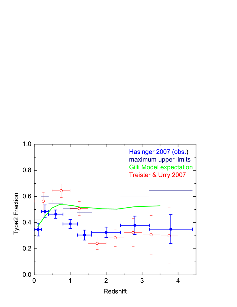
Figure 6: The observed fraction of type–2 AGN as a function of redshift. Filled Symbols and horizontal upper limits are from [Hasinger 2007], open symbols from [Treister & Urry 2006]. The solid line shows the prediction of the [Gilli et al. 2007] model, assuming no obscuration evolution (courtesy: Roberto Gilli).

Figure 6 is integrated over all luminosities in each redshift shell and therefore possibly hiding trends, which are observable in a better resolved parameter space. In figure 7 we therefore finally show the type–2 fraction as a function of luminosity, determined in the different redshift shells and compared to the mean relation in the $z=0.2-3.2$ interval. A similar decreasing type–2 fraction as a function of luminosity is found in each redshift interval. At closer look, there is however a small trend of increasing obscuration fraction with redshift, even ignoring the lowest redshift shell, which is affected most by the flux limit incompleteness (see figure 6). A more quantitative analysis will be shown in Hasinger (2007).

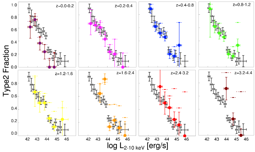
Figure 7: Type-2 fraction as a function of X–ray luminosity in different redshift shells. Filled circles show the data in the individual redshift shell indicated on each panel, while crosses give the average relation in the z=0.2-3.2 range for comparison.

3 The cosmic X–ray background

One major goal in X–ray astronomy is to explain the origin of the cosmic background emission in detail. The observed emission in X–rays originates mainly from AGN (point sources) and galaxy clusters (extended sources) ([Giacconi et al. 1962, Hasinger 2004, Brandt & Hasinger 2005]). Figure 8 displays the typical appearance of an XMM–Newton X–ray deep field, located in the Lockman Hole in this case ([Hasinger et al. 2001]). The Lockman Hole is an extraordinary location at the sky due to the fact that the column density is very low, $N_{\rm H}=5.7\times 10^{19}\ {\rm cm}^{-2}$ ([Lockman et al. 1986]).

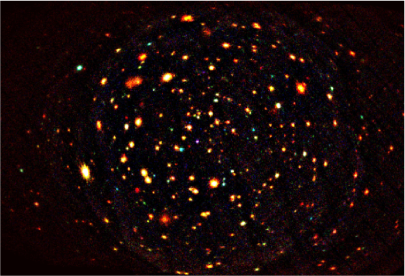
Figure 8: X–ray deep field image taken in the Lockman Hole with XMM–Newton ([Hasinger et al. 2001]). The total exposure time amounts to $\sim$800 ks. This is a X–ray false colour composite image with red, green, and blue corresponding to 0.5-2, 2-4.5 and 4.5-10 keV photon energy. Point–like and extend sources are clearly visible that are associated with AGN and galaxy clusters respectively.

Different groups developed detailed population synthesis models to reconstruct the observed cosmic X–ray background (XRB). Highly obscured AGN turn out to be crucial in this modelling. Even in the local universe, it has been shown that $\simeq$40% of the Seyfert galaxies are Compton–thick ([Risaliti et al. 1999]). This means that these sources are missing from all current X–ray surveys because their column density is extremely large, $\log N_{\rm H}\gtrsim 25$. As a consequence, only the reflected emission is seen in these X–ray spectra. This hidden AGN population should show up in mid–infrared surveys. The flux criterion $F_{E>10\,{\rm keV}}\gg F_{\rm SX}$ may serve as another good indicator for Compton–thick sources that could be investigated with INTEGRAL or Swift. Recently, [Ueda et al. 2007] have presented Suzaku observations of two AGN out of a small sample detected in the Swift BAT survey, which show substantial X–ray absorption and may well be moderately obscured Compton-thick objects. Based on Chandra data from the CDF–S, Tozzi et al.(2006) have found $\simeq$5% of AGN are Compton–thick and in the XMM–Newton observations of the COSMOS field a similar fraction of candidate Compton–thick AGN is found ([Hasinger et al. 2006]). Beyond $z\simeq 0.1$ Compton–thick AGN are, however, very sparse ([Martinez–Sansigre et al. 2006]).

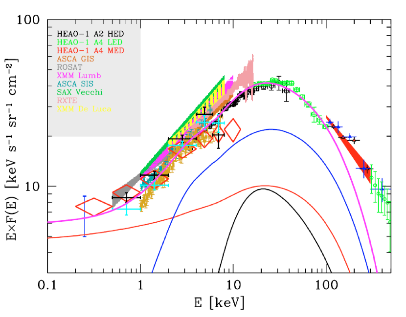
Figure 9: The observed cosmic XRB spectrum (data points) and the predicted contributions of different AGN families (solid lines) taken from [Gilli et al. 2007]. Total AGN plus galaxy clusters, type–2 Compton–thin AGN, type–1 Compton–thin AGN and type–2 Compton–thick AGN are drawn as solid lines (from top to bottom). Only the three populations together fit the observed XRB spectrum well. Compton–thin AGN contribute most.

Recently, a new self–consistent population synthesis model for the cosmic X–ray background has been developed ([Gilli et al. 2007]), including the most recent determination of the AGN luminosity function evolution in the soft and hard X–ray bands. Gilli et al.  consider a $N_{\rm H}$ distribution with a relatively small fraction of unabsorbed AGN ($\log N_{\rm H}<22$) but with a growing contribution at higher column densities. Most of the emission originates from the Compton–thin AGN population. For the spectral templates a more complex model is assumed: The spectral index of the sources scatters in a Gaussian fashion around an average value of $<\Gamma>=1.9$. Such spectral templates increase the contribution of Compton–thin AGN at 30 keV in the background spectrum by 30% (as compared to $\Gamma=const$ templates). However, the observed background spectrum still calls for a moderatly and heavily obscured Compton–thick AGN population that contributes significantly around 30 keV. Moderatly obscured Compton-thick AGN have $24<\log N_{\rm H}<25$ whereas heavily obscured Compton-thick AGN have $\log N_{\rm H}>25$. To date only $\simeq$40 local sources are candidates for Compton–thick AGN [(Comastri 2004)]. However, the Compton–thick AGN are expected to become very numerous below current flux limits. This fact motivates for intensive studies with future X–ray missions such as Simbol–X, Spectrum–X-Gamma, NeXT, Constellation–X and XEUS.

Figure 9 shows the results from the most recent population synthesis model (Gilli et al. 2007). The model involving three AGN populations (unabsorbed Compton–thin, absorbed Compton–thin and Compton–thick sources) is in good agreement with the observed data points. Note that only the inclusion of the Compton–thick population (lowest bump peaking around 20-30 keV) reproduces the total cosmic XRB spectrum. The fraction of Compton–thick AGN predicted by this model is consistent with the actually observed numbers in the Swift BAT, INTEGRAL and CDF–S catalogues.

4 Conclusions

The major scientific topic of this spring symposium are black holes. Many theoretical contributions have been presented at the meeting that help in understanding these mysterious objects. In contrast, X–ray astronomy offers the possibility to study black holes in action. Together with gravitational waves X–rays are best suited because they allow insight into the direct surroundings of black holes.

This review demonstrates that X–ray astronomy is a powerful tool to understand black hole activity and their cosmological role in galaxy formation and galaxy evolution. Deep X–ray surveys probe black holes at cosmological distances. It is crucial to determine the redshift of these sources to trace back their cosmic history. This is done by optical follow–up observations with the best telescopes worldwide. Many X–ray surveys together provide a highly complete data set which can be exploited scientifically.

The most relevant findings of recent AGN X–ray cosmology are the following:

1. Observed X–ray spectra support the standard model of AGN, that is an accreting SMBH. However, AGN unification schemes have to consider luminosity effects and feedback mechanisms.

2. The cosmic X–ray background is a total signal of individual active galaxies and galaxy clusters.

3. An AGN classification scheme requires both optical (broad vs. narrow emission lines) and X–ray (absorbed versus unabsorbed spectrum) information.

4. The fraction of type–2 to type–1 AGN decreases with luminosity. This indicates an interaction between the luminous galactic nucleus and its environment. Luminous AGN seem to be able to clean out their environment.

5. The type–2 fraction shows a small evolution with redshift in the sense that higher redshift environments seem to have somewhat more absorption.

6. Active galaxies do not evolve in a uniform manner. Depending on the luminosity (or black hole mass respectively) SMBHs exhibit an anti–hierarchical growth, i.e. quasars enter the cosmic stage significantly earlier than Seyfert galaxies. In other words: the density evolution of AGN is luminosity–dependent.

7. X–ray luminosity functions are in perfect agreement with other wavebands.

8. Compton–thin AGN contribute most to the cosmic X–ray background.

9. However, Compton–thick AGN are an essential ingredient to reproduce the total cosmic X–ray background spectrum. They mainly contribute at photon energies around 30 keV.

10. Accreted BHMFs from the X–ray background can be reconciled with dormant relic BHs in the local universe if one assumes that the BHs rotate.

11. Theory and observation indirectly support the existence of progenitors such as mini–quasars at $z\simeq 11$ and GRBs at $z\simeq 20$. This should be tested by direct observations with XEUS.

X–ray astronomy is going to be successful in future if the survey capacities are extended successively. Surveys with larger fields and deeper pencil beams are natural goals. Therefore, upcoming projects such as eRosita aboard Spectrum–X–Gamma, Simbol–X, NeXT and XEUS are promising scientific drivers.