Time reversal Aharonov-Casher effect in mesoscopic rings with Rashba spin-orbital interaction

Abstract

The time reversal Aharonov-Casher (AC) interference effect in the mesoscopic ring structures, based on the experiment in Phys. Rev. Lett. 97, 196803 (2006), is studied theoretically. The transmission curves are calculated from the scattering matrix formalism, and the time reversal AC interference frequency is singled out from the Fourier spectra in numerical simulations. This frequency is in good agreement with analytical result. It is also shown that in the absent of magnetic field, the Altshuler-Aronov-Spivak type (time reversal) AC interference retains under the influence of strong disorder, while the Aharonov-Bohm type AC interference is suppressed.

The advancement of spintronics and spintronic materials has provided opportunities to study and utilize new electronic devices based on the electron spin degrees of freedomspin . The novel spin related properties can be detected by tuning the spin-orbital interaction (SOI). Phenomena related to Rashba effects in, e.g., InAs and In_1-xGa_xAs based two-dimensional electron gas (2DEG) systems have been observedsato ; nitta . The value of the Rashba parameter in these semiconductor systems can be as high as $4\times 10^{-11}$eVm. The experimental resultssato ; nitta have shown that in InAs and In_1-xGa_xAs based 2DEG systems, the Rashba effect is responsible for the spontaneous spin splitting. Many advanced electronic devices have been proposed to manipulate electron spin, such as spin transistordatta , waveguideswang ; sun , spin filterskoga , spin interferometersNitta1 ; shen , etc. In the spin interference deviceNitta1 ; shen ; frus , the resistance is adjusted via the gate voltage using the spin interference phenomenon of the electronic wave functions in a mesoscopic ring. In the presence of Rashba SOIRashba , the wave function acquires the Aharonov-Casher (AC) phase when an electron moves along the ringAC1 ; AC2 . If the quantum coherence length is larger than or comparable with the electron mean free path, the resistance amplitude will depend on the AC phases of electron wave functions in the two arms of the ring and display interference pattern. Meanwhile, the modulation of interference with the aid of AC phase could be further tuned through an applied gate voltagenitta .

The experimental demonstrations of the spin interference in the AC rings have been reported recentlyKonig ; bergsten . As expected, the resistance of the ring oscillates with the gate voltage and an external magnetic field. However, their experimental results do not directly establish the time reversal AC frequency. In this study, we numerically investigate the transport properties of multi mesoscopic rings with magnetic field and Rashba SOI in the framework of Landauer-Büttiker formalism. The interference modes are analyzed by means of the fast Fourier transformation (FFT) algorithm. As a subsidiary interference, the magnetic flux leads to the conventional Aharonov-Bohm (AB) AB1 and Altshuler-Aronov-Spivak (AAS) AAS1 ; AAS2 effects. Subtracting the contribution of magnetic flux and determining the pathes of electrons from the frequency spectra, AB and AAS type oscillations associated with SOI in rings are confirmed. In the presence of dephasing, AAS type (time reversal) AC interference remains, while the AB type oscillation is suppressed.

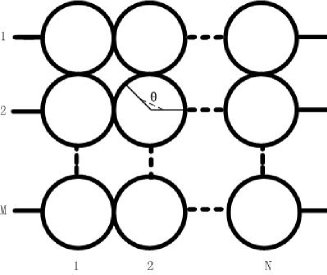
Figure 1: The schematic graph of the M-N ring-array structure. The dot lines represent the omitted rings. $\theta$ is the local polar coordinates.

The M-N ring-array structure, as shown in Fig. 1, mimics the experimental configurations bergsten . For simplicity, each arm of the ring is assumed to be a one-dimensional (1D) quantum wire and connected with each other at crossing points. The $2M$ leads are connected to the M-N ring-array as $M$ 1D-channels. The external magnetic and electric fields are perpendicular to the plane of the rings. The system can be solved by dividing it into several sections, i.e., the semi-infinite left M-leads, the region of M-N rings array in the presence of SOI, and the semi-infinite right M-leads. With the continuity condition on the boundaries between sections, the scattering matrix formalismandreas can be established.

Because of the absence of the SOI in the leads, the wavefunction in the left (right) i-th channel can be written in the form of $\psi_{iL}=a_{iL,+}e^{ikx}|\uparrow>+a_{iL,-}e^{ikx}|\downarrow>+b_{iL,+}e^{-ikx}|\uparrow>+b_{iL,-}e^{-ikx}|\downarrow>$ and $\psi_{iR}=a_{iR,+}e^{ikx}|\uparrow>+a_{iR,-}e^{ikx}|\downarrow>$ for an incident electron with momentum $\hbar k$. The coefficients satisfy the condition $\sum_{i\sigma=\pm}\left|b_{iL,\sigma}\right|^{2}+\sum_{i\sigma=\pm}\left|a_{iR,\sigma}\right|^{2}=\sum_{i\sigma=\pm}\left|a_{iL,\sigma}\right|^{2}=1$.

In the region of M-N rings array, the electronic wavefunction $\Psi$ in the rings can be expanded in terms of the complete set of eigenfunctions $\psi_{n\sigma}\left(\theta\right)$ as $\Psi_{ij}\left(\theta;k\right)=\sum_{n\sigma}c_{n\sigma}\psi_{n\sigma}\left(\theta;k\right)$ with the spin index $\sigma$ for the ring (i, j). For a single ring, the Hamiltonian in the local polar coordinates readsHamiltonian

$$H = \frac{\hbar^{2}}{2m^{\ast}r^{2}}\left(-i\partial_{\theta}+\frac{\Phi}{\Phi_{0}}\right)^{2}+\frac{\alpha}{2r}\left(\begin{array}[]{cc}0&-e^{-i\theta}\\ e^{i\theta}&0\end{array}\right)$$ (6)

$$+\frac{\alpha}{r}\left(\begin{array}[]{cc}0&e^{-i\theta}\\ e^{i\theta}&0\end{array}\right)\left(-i\partial_{\theta}+\frac{\Phi}{\Phi_{0}}\right)$$

(Here $m^{\ast}$ is the electron effective mass and we take $m^{\ast}=0.05m$, $r$ is the radius of a single ring, $\alpha$ is the Rashba SOI strength, and $\Phi$ is the magnetic flux in unit of the flux quanta $\Phi_{0}=h/e$. We ignore the Zeeman terms because of the weak magnetic field, and concentrate on the effect generated by SOI.) The eigenfunctions of the system are $\psi_{n,+}\left(\theta\right)=\left(2\pi\right)^{-1/2}e^{in\theta}\left(\cos\beta/2,-e^{i\theta}\sin\beta/2\right)^{T}$, $\psi_{n,-}\left(\theta\right)=\left(2\pi\right)^{-1/2}e^{in\theta}\left(\sin\beta/2,e^{i\theta}\cos\beta/2\right)^{T}$, and the corresponding eigenvalues are $\epsilon_{n,\pm}=\left(\hbar^{2}/2m^{\ast}r^{2}\right)\left[\left(n+\Phi/\Phi_{0}\right)^{2}+\left(2n+2\Phi/\Phi_{0}+1\right)\Omega_{\pm}\right]\mp\left(\alpha/2r\right)\left(2n+2\Phi/\Phi_{0}+1\right)\sin\beta$, with $\tan\beta=2mr\alpha/\hbar^{2}$, $\Omega_{\pm}=-1/2\left(1\pm\cos\beta\right)$, and $T$ denotes the transposition of vectors.

The linear equations among coefficients $c_{n\sigma}$ can be determined by the Griffith conditions Griffith at each joint point. After obtaining the sets of wavefunctions $\psi_{iL}$, $\psi_{iR}$ and $\Psi_{ij}\left(\theta;k\right)$, the scattering matrices can be derived according to the multi-mode scattering-matrix procedure given in Ref. andreas . Therefore, the total transmission and reflection coefficients of ring-array system can be obtained.

We have calculated the transmission coefficients for several ring-array systems under different magnetic flux $\Phi$ and Rashba coefficient $\alpha$. The phenomena are similar in the systems with different number of rings and radii, and we take the 3-3 ring-array with $r=1\mu$m as a special case to display our results. In Fig. 2(a), we present the transmission coefficient versus magnetic flux ($T$ vs $\Phi$) of the 3-3 ring-array with the electronic incident wavevector $k=1.009651\times 10^{8}$m^-1 and the Rashba coefficient $\alpha=2$peVm. The transmission coefficient oscillates with the magnetic flux periodically. Although the shapes of the curves may look quite different with different $k$ and $\alpha$, the periods of the curves are the same. In fact, as we can see in the right panel, the FFT spectra of the curve reveals different interference modes (namely AB, AAS, etc.). For various systems with different $k$ and $\alpha$, the FFT spectra of the $T$ vs $\Phi$ curves include the same modes, but the amplitude of these modes will be different.

In the absence of magnetic flux, transmission $T$ oscillates with tuning the SOI strength [Fig. 2(b)]. The oscillation is no longer strictly periodic at large incident electron momentum, because of the complicated back and forth multi-scattering between channels and rings. However, the Fourier spectra still reveal the same main frequency at $\alpha^{-1}=0.646$ $\left(\text{peVm}\right)^{-1}$, which corresponds to the AB type oscillation. Besides this mode, other modes at $\alpha^{-1}=1.312$ $\left(\text{peVm}\right)^{-1}$, $...$ (AAS type etc.), are not very clear here. While in the case for a single AC ring, these modes will be clearly shown in the FFT spectra.

The frequencies subsumed in the Fourier spectra on the right panels of Fig. 2(b) can be understood analytically from a single ring structure. The AC phase difference of opposite spins traveling in full counter-clockwise (CCW) and clockwise (CW) circle are given by frus $\Delta\varphi_{\psi_{-}^{\downarrow}-\psi_{+}^{\uparrow}}=2\pi\left[1+\sqrt{1+\left(2rm^{\ast}\alpha/\hbar^{2}\right)^{2}}\right]$ and $\Delta\varphi_{\psi_{-}^{\uparrow}-\psi_{+}^{\downarrow}}=2\pi\left[1-\sqrt{1+\left(2rm\alpha/\hbar^{2}\right)^{2}}\right]$. In the limit of large $\alpha$, the two phase differences take the same form as in Ref.Nitta1 ; Konig . Therefore, the AAS oscillation amplitude can be expressed as Nitta3

$$\delta R_{\alpha}^{AAS}=\delta R_{\alpha=0}\cos\left[2\pi\sqrt{1+\left(\frac{2rm^{\ast}\alpha}{\hbar^{2}}\right)^{2}}\right].$$ (7)

From this relation the AAS type (time reversal) AC frequency is approximately at $\alpha_{AAS}^{-1}=2rm^{\ast}/\hbar^{2}=1.31$peVm, while the AB type oscillation frequency is $\alpha_{AB}^{-1}=rm^{\ast}/\hbar^{2}=0.65$peVm, as indicated in the Fourier spectrum.

Figure 2: (a) The curves for T vs $\Phi$ and the corresponding Fourier spectrum for 3-3 ring-array with $k=1.009651\times 10^{8}m^{-1}$ and $\alpha=2peVm$; (b) The curves for T vs $\alpha$ and the corresponding Fourier spectrum for 3-3 ring-array with $k=1.009651\times 10^{8}m^{-1}$ and $\Phi=0$.

In order to emphasize on the AAS effect in the ring structure and bring light to the objective law governing the spin interference, we introduce disorder induced dephasing effect, so that the AB type oscillation is suppressed. For simplicity, a single ring with two leads is considered, which is enough to manifest the main principle of AAS effect in a ring structure. The conductance is numerically calculated with a tight-binding model. The tight-binding Hamiltonian for a ring in Eq. (1) is given bynikolic

$$H = \sum_{l=1}^{N}\sum_{\sigma=\uparrow\downarrow}\epsilon_{l}c_{l\sigma}^{{\dagger}}c_{l\sigma}-\sum_{l=1}^{N}\sum_{\sigma=\uparrow\downarrow}(tc_{l\sigma}^{{\dagger}}c_{l+1\sigma}+h.c.)$$

$$-\sum_{l=1}^{N}[i\lambda(e^{-i\varphi_{l}}c_{l,\uparrow}^{{\dagger}}c_{l+1,\downarrow}+e^{i\varphi_{l}}c_{l,\downarrow}^{{\dagger}}c_{l+1,\uparrow})+h.c.],$$

where $\epsilon_{l}$ is the lattice on site energy, the operator $c_{l,\sigma}^{{\dagger}}(c_{l,\sigma})$ creates (annihilates) an electron with spin $\sigma$ at site $l$, $N$ is the total number of lattices in the ring, and $\varphi_{l}=\pi(2l-1)/N$ as defined in Ref. nikolic . The hopping coefficients in the second and third summations can be expressed as $t$ (and $\lambda$) $=t_{0}$ (and $\lambda_{0}$) $\exp(ie\Phi/\hbar N)$ and $t_{0}\equiv\hbar^{2}/2m^{\ast}a^{2}$ is the nearest neighbor hopping element with lattice spacing $a$ along the 1D ring. $\lambda_{0}=\alpha/2a$ describes the strength of the Rashba SO interaction. $\Phi$ is the magnetic flux through the 1D ring. In our numerical calculations, $\epsilon_{l}=0$ if disorder potential at each site is absent, otherwise, the lattice on site energy $\epsilon_{l}$ is generated by a uniform distribution $[-w/2,w/2]$ of disorder strength $w$. Because of the periodic boundary condition, $c_{N+1,\sigma}^{{\dagger}}$ ($c_{N+1,\sigma}$) is identical as $c_{1,\sigma}^{{\dagger}}(c_{1,\sigma})$. In addition, two semi-infinite 1D leads are attached to the 1D ring to make sure that the upper and lower arms have the same length. The influence of these two leads is taken into account through self-energy terms. The conductance is calculated numerically as outlined in Ref. AC4 .

For a certain Fermi energy and Rashba SOI strength, the conductance of 3-3 rings array exhibits the periodic oscillation as a function of the magnetic flux $\Phi$. FFT analysis displays AB, AAS, and other higher frequencies as shown in Fig. 2(a). However, as we will show below, with the increasing of the disorder strength $w$, the AB oscillation is suppressed and only the time reversal AAS oscillation amplitude remains. Similar results have been reached in a 1D square loop system AC4 .

To see the suppression of AB type oscillation in the presence of disorder, the conductance is calculated for a single 1D ring with different Rashba SOI strengths. Employing FFT and inverse FFT techniques, we first calculate the flux dependent conductance and then extract the AAS oscillation amplitudes at zero magnetic field for a series of different $\lambda_{0}$. Afterwards we retrieve the information about AAS oscillation amplitudes vs $\lambda_{0}$ (same steps as in Ref. bergsten ). The purpose of this approach is to single out the time reversal AC phase differences. Under the influence of magnetic field and Rashba SOI, two paths will accumulate both AB and AC phases before interference. Since AAS oscillation is caused by the interference of two time reversal paths (one CCW circle and another CW circle), it is feasible to find out AC phase difference between these two time reversal paths, if we extract AAS oscillation and set magnetic field to be zero.

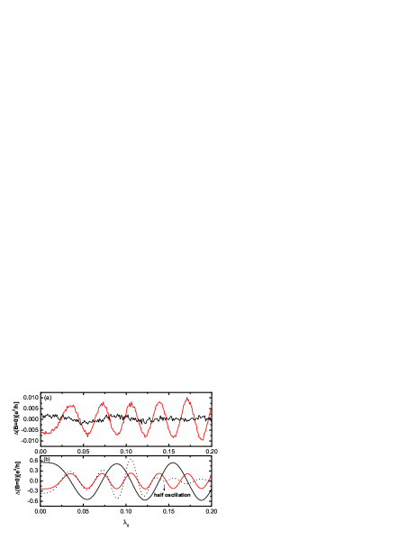
Figure 3: The AAS and AB oscillation amplitudes versus $\lambda_{0}$ curves are drawn in red and black solid line respectively, for a single 1D ring (a) under disorder average with $w=0.8$, $E_{f}=-1.8$ and (b) under Fermi energy average. The AAS oscillation amplitudes versus $\lambda_{0}$ at $E=-1.8$ (black dotted line) has also been plotted for comparisons in (b). Other parameters are set as $N=100$, $t_{0}=1$. All the energies are measured in the units $t_{0}$.

Fig. 3(a) shows the AAS oscillation amplitude versus $\lambda_{0}$ curves (red solid lines) and the AB oscillation amplitude versus $\lambda_{0}$ curves (black solid lines) under disorder average with disorder strength $w=0.8$. Compared with the AAS oscillation, the AB oscillation has been suppressed greatly under the disorder average.

While Fig. 3(b) shows the AAS oscillation amplitude versus $\lambda_{0}$ curves (red solid lines) and the AB oscillation amplitude versus $\lambda_{0}$ curves (black solid lines) under average over incident electron energy (Fermi energy). In this case, the AB oscillation has not been suppressed. Besides, although these two kinds of averages lead to the similar AAS oscillation shapes in the conductance, the oscillation amplitude under the disorder average is almost 20 times smaller than that of energy average case. The suppression of the amplitude is due to the fact that electron will be localized at large disorder strength.

In these plots, no trace of half oscillation, which appears in the experimental resultsbergsten , could be found. However, from the AAS oscillation amplitudes versus $\lambda_{0}$ for a single 1D ring at $E=-1.8$ [dotted line in Fig. 3(b)], we notice that the so-called ”half oscillation” appears indeed as the experimentsbergsten . In comparison of the AAS oscillation amplitude versus $\lambda_{0}$ for $E=-1.8$ and under Fermi energy average, it is shown that at the strength of SOI where the half oscillation happened, the following oscillation amplitude differs a phase shift $\pi$ with the energy averaged oscillation amplitude. When $\lambda_{0}$ is smaller than 0.145 (before half oscillation), the peak and dip features of these two curves match well with each other. But when $\lambda_{0}$ is larger than 0.145, the peak feature of one curve corresponds to the dip feature of another. These conclusions can also be inferred from the experimentbergsten . Therefore, we conclude that half oscillation only happens at some certain Fermi energy (carrier density). But this behavior disappears after ensemble average (disorder or Fermi energy average).

Figure 4: The conductance of a single 1D ring versus $\lambda_{0}$ without magnetic field. (a), (b) are calculated from $E_{f}=-0.05$ with disorder strength $w=0,1.5$ respectively. (c) is calculated from Fermi energy average without disorder. All the corresponding FFT spectrum are shown on the right side. The size of the ring N=100. The theoretical time reversal (AAS type) AC frequency is at $\lambda_{0}^{-1}=31.83$. In our FFT spectrum, the AAS type AC frequency is located at $\lambda_{0}^{-1}=29.30$.

From the FFT spectrum of AAS oscillation amplitude versus $\lambda_{0}$ curves [red curves in Fig. 3(a) and 3(b)], we find a frequency peak located at $\lambda_{0}^{-1}=31.25$. From the theoretical time reversal AC frequency $\alpha^{-1}=2rm^{*}/\hbar^{2}$, we get $\lambda_{0}^{-1}=N/\pi$. Thus the theoretical time reversal AC frequency should be $\lambda_{0}^{-1}=31.83$ for N=100. Comparing these two values, our numerical result agrees well with the theoretical value.

Finally, in order to substantiate our conclusion, we plot the conductance versus $\lambda_{0}$ in absent of magnetic field for several cases: without disorder, with disorder average and with energy average (Fig. 4). From their FFT spectra, it is seen that different oscillation frequencies are included when disorder is absent [Fig. 4(a)]. With strong disorder strength, the AB type component is suppressed [Fig. 4(b)]. Thus, we are sure that the time reversal AC effect have been successfully demonstrated in such a system. However, the case of Fermi energy average is quite different from disorder average. In the FFT spectrum of energy average [Fig. 4(c)], other oscillation frequencies (two half circle interference …) can not be smeared out under energy average. The AB oscillation amplitude at zero magnetic field becomes smaller with increasing disorder strength, but it still remains strong under Fermi energy average, which supports our conclusion in Fig. 3.

In summary, we have numerically demonstrated the time reversal AC interference effect in mesoscopic rings. In the absent of disorder, various AC interference patterns are included in the rings. Nevertheless, most interference modes are weak against disorder, except the time reversal mode.

- (1) I. Zutic, J. Fabian, and S. Das Sarma, Rev. Mod. Phys. 76,323 (2004).
- (2) Y. Sato, T. Kita, S. Gozu, and S. Yamada, J. Appl. Phys. 89, 8017 (2001); D. Grundler, Phys. Rev. Lett. 84, 6074 (2000).
- (3) J. Nitta, T. Akazaki, H. Takayanagi and T. Enoki, Phys. Rev. Lett. 78, 1335 (1997).
- (4) B. Datta and S. Das, Appl. Phys. Lett. 56, 665 (1990).
- (5) X. F. Wang, P. Vasilopoulos, and F. M. Peeters, Phys. Rev. B 65, 165217 (2002).
- (6) Q. F. Sun and X. C. Xie, Phys. Rev. B 71, 155321 (2005); Q. F. Sun and X. C. Xie, ibid. 73, 235301 (2006).
- (7) T. Koga, J. Nitta, H. Takayanagi, and S. Datta, Phys. Rev. Lett. 88, 126601 (2002).
- (8) J. Nitta, F. E. Meijer and H. Takayanagi, Appl. Phys. Lett. 75, 695 (1999).
- (9) S-Q Shen, Z-J Li and Z-S Ma, Appl. Phys. Lett. 84, 996 (2004).
- (10) D. Frustaglia and K. Richter, Phys. Rev. B 69, 235310 (2004).
- (11) Y. A. Bychkov and E. I. Rashba, J. Phys. C 17, 6039 (1984).
- (12) Y. Aharonov and A. Casher, Phys. Rev. Lett. 53, 319 (1984).
- (13) T-Z Qian and Z-B Su, Phys. Rev. Lett. 72, 2311 (1994).
- (14) M. Konig, A. Tschetschetkin, E. M. Hankiewicz, J. Sinova, V. Hock, V. Daumer, M. Schafer, C. R. Becker, H. Buhmann and L. W. Molenkamp, Phys. Rev. Lett. 96, 076804 (2006).
- (15) T. Bergsten, T. Kobayashi, Y. Sekine and J. Nitta, Phys. Rev. Lett. 97, 196803 (2006).
- (16) Y. Ahronov and D. Bohm. Phys. Rev. 115, 485 (1959).
- (17) B. L. Al’tshuler, A. G. Aronov and B. F. Spivak, JETP Lett. 33, 94 (1981).
- (18) D. Yu Sharvin and Yu V.Sharvin. JETP Lett. 34, 272 (1981).
- (19) A. Weisshaar, J. Lary, S. M. Goodnick and V. K. Tripathi, J. Appl. Phys. 70, 355 (1991).
- (20) F. E. Meijer, A. F. Morpurgo and T. M. Klapwijk, Phys. Rev. B 66, 033107 (2002).
- (21) S. Griffith, Trans. Faraday Soc. 49, 345 (1953).
- (22) M. J. van Veenhuizen, T. Koga and J. Nitta, Phys. Rev. B 73, 235315 (2006).
- (23) S. Souma and B. K. Nikolic, Phys. Rev. B 70, 195346 (2004).
- (24) Z. Zhu, Q-F Sun, B. Chen and X. C. Xie, Phys. Rev. B 74, 085327 (2006); S. G. Cheng, Q-F Sun, and X. C. Xie, J. Phys. C 18, 10553 (2006).