Padé approximants of random Stieltjes series

Abstract.

We consider the random continued fraction

$$S(t):=\cfrac{1}{s_{1}+\cfrac{t}{s_{2}+\cfrac{t}{s_{3}+\cdots}}}\,,\quad t\in{\mathbb{C}}\backslash{\mathbb{R}}_{-}\,,$$

where the $s_{n}$ are independent random variables with the same gamma distribution. Every realisation of the sequence defines a Stieltjes function that can be expressed as

$$S(t)=\int_{0}^{\infty}\frac{\sigma(\text{\rm d}x)}{1+xt}\,,\quad t\in{\mathbb{C}}\backslash{\mathbb{R}}_{-}\,,$$

for some measure $\sigma$ on the positive half-line. We study the convergence of the finite truncations of the continued fraction or, equivalently, of the diagonal Padé approximants of the function $S$. By using the Dyson–Schmidt method for an equivalent one-dimensional disordered system, and the results of Marklof et al. (2005), we obtain explicit formulae (in terms of modified Bessel functions) for the almost-sure rate of convergence of these approximants, and for the almost-sure distribution of their poles.

1. Introduction

Let $\mathbf{s}=(s_{1},s_{2},\ldots)$ be a sequence of positive real numbers and consider the analytic continued fraction

(1.1) $$S(t):=\cfrac{1}{s_{1}+\cfrac{t}{s_{2}+\cfrac{t}{s_{3}+\cdots}}}\,,\quad t\in{\mathbb{C}}\backslash{\mathbb{R}}_{-}\,.$$

This continued fraction defines a Stieltjes function; it can be represented in integral form as

(1.2) $$S(t)=\int_{0}^{\infty}\frac{\sigma(\text{\rm d}x)}{1+tx}$$

for some measure $\sigma$ supported on the non-negative half-line such that the moments

(1.3) $$m_{n}:=\int_{0}^{\infty}x^{n}\sigma(\text{\rm d}x),\quad n\in{\mathbb{N}},$$

exist. By an obvious use of the geometric series, every Stieltjes function can be expanded formally in powers of $t$:

(1.4) $$S(t)\sim\sum_{j=0}^{\infty}m_{j}\,(-t)^{j}\quad\text{as $t\rightarrow 0+$}\,.$$

Hence $S$ is the moment generating function of the measure $\sigma$. It is a well-known fact of great practical importance that, given the first $n$ of the moments, one may construct the rational function

(1.5) $$S_{n}(t):=\frac{P_{n}(t)}{Q_{n}(t)}=\cfrac{1}{s_{1}+\cfrac{t}{s_{2}+\cdots+\cfrac{t}{s_{n}}}}\,,\quad t\in{\mathbb{C}}\backslash{\mathbb{R}}_{-}\,,$$

where

$$\deg P_{n}=\begin{cases}n/2-1&\text{if $n$ is even}\\ (n-1)/2&\text{if $n$ is odd}\end{cases}\quad\text{and}\quad\deg Q_{n}=\begin{cases}n/2&\text{if $n$ is even}\\ (n-1)/2&\text{if $n$ is odd}\end{cases}\,.$$

This truncation of the continued fraction (1.1) has a MacLaurin expansion whose $n$th partial sum agrees with that of the series (1.4). Hence $S_{n}$ is a diagonal (if $n$ is odd), or near-diagonal (if $n$ is even) Padé approximant of $S$.

Now suppose that the $s_{n}$ are independent positive random variables with the same distribution, say $\mu$. We shall consider the following questions:

1. What are the almost-sure analytic properties of these Stieltjes functions?

2. What is the almost-sure leading asymptotic behaviour of the error $S(t)-S_{n}(t)$ as $n\rightarrow\infty$?

These questions are of interest because Padé approximation is widely used in applied mathematics as a practical means of accelerating the convergence of the partial sums of series obtained by perturbation methods. As pointed out by Bender & Orszag (1978), the consideration of many particular cases where the $s_{n}$ are deterministic reveals a wide range of large-$n$ behaviours. Our motivation for studying the random case is to gain some insight into the asymptotic behaviour of Padé approximation in the “generic” case.

Our study of diagonal Padé approximation reduces to aspects of the large-$n$ behaviour of the denominators $Q_{n}$. For this reason, as in the deterministic case, the cornerstone of the analysis is the three-term recurrence relation

(1.6) $$Q_{n+1}=tQ_{n-1}+s_{n+1}Q_{n}\,,\quad Q_{-1}=0,\;\;Q_{0}=1\,.$$

(The $P_{n}$ satisfy the same recurrence relation, albeit with different initial conditions.) This recurrence relation makes a link between Padé approximation and a rich set of other mathematical entities, such as orthogonal polynomials, products of random matrices, and discrete Schrödinger-like operators. By exploiting results that are well-known in these related fields, one may obtain— for a very large class of distributions $\mu$ of the coefficients $s_{n}$— some partial answers to the questions stated earlier. Our contribution in the present paper is to elaborate the particular case where $\mu$ is the gamma distribution. More precisely, we obtain explicit formulae (in terms of Bessel functions) for the leading term in the asymptotic behaviour of the error of Padé approximation and for the asymptotic distribution of the poles, as well as the location of the essential spectrum of the measure $\sigma$.

In the remainder of this introductory section, we describe briefly the key ideas underlying the analysis. Then we summarise our main results in the form of a theorem.

1.1. The moment problem

The Stieltjes moment problem is, given a sequence $\{m_{n}\}_{n\in{\mathbb{N}}}$, to determine whether or not there exists a measure $\sigma$ such that equation (1.3) holds for every $n$. Historically, mathematical objects such as the analytic continued fraction (1.1), orthogonal polynomials and Padé approximants were introduced as tools in the study of this moment problem (Akhiezer 1961; Nikishin & Sorokin 1988; Simon 1998). Stieltjes (1894) showed that a necessary and sufficient condition for the existence of a measure $\sigma$ with the prescribed moments is

(1.7) $$\forall\;n\in{\mathbb{Z}}_{+}\,,\quad s_{n}>0\,.$$

He also showed that

(1.8) $$\sum_{n=1}^{\infty}s_{n}=\infty$$

is a necessary and sufficient condition for the uniqueness of the measure.

Let us assume that condition (1.7) holds and describe in very broad terms one way of “reconstructing” $\sigma$ from its moments; see Akhiezer (1961) and Nikishin & Sorokin (1988) for a detailed treatment.

Recall that $x^{\prime}$ is a point of increase of the measure $\sigma$ if

$$\forall\;\varepsilon>0,\quad\int_{\max\{x^{\prime}-\varepsilon,0\}}^{x^{\prime}+\varepsilon}\sigma(\text{\rm d}x)>0\,.$$

The spectrum of $\sigma$ is the set of its points of increase and will be denoted $\text{spec}(\sigma)$. For $x>0$, we shall denote by $\delta_{x}$ the probability measure on ${\mathbb{R}}_{+}$ whose only point of increase is $x$.

Given the $m_{n}$, we may define an inner product, say $(\cdot,\cdot)_{\mathbf{m}}$, on the space of polynomials as follows: if $p$ and $q$ are two polynomials with coefficients $p_{i}$ and $q_{i}$ respectively, then

$$(p,q)_{\mathbf{m}}:=\sum_{i,j}m_{i+j}\,p_{i}\,q_{j}\,.$$

Knowing the moments, we may compute the $s_{n}$ and the $S_{n}$. We remark that $P_{2n}$ and $Q_{2n}$ are polynomials of degree $n-1$ and $n$ respectively. Set

(1.9) $$\psi_{n}(\lambda):=\sqrt{s_{2n+1}}\,\lambda^{n}Q_{2n}(-1/\lambda)\,.$$

Then the fact that $S_{2n}$ matches the moment generating series to $O(t^{2n})$ implies that $\psi_{n}$ is orthogonal to every polynomial of degree less than $n$, in the sense of the inner product $(\cdot,\cdot)_{\mathbf{m}}$. It follows (see Akhiezer 1961, Chapter 1) that the roots of $\psi_{n}$ are simple and lie in ${\mathbb{R}}_{+}$; denote them by

$$0\leq\lambda_{n,1}<\lambda_{n,2}<\cdots<\lambda_{n,n}<\infty\,.$$

Gaussian quadrature then defines a discrete measure

(1.10) $$\sigma_{n}:=\sum_{j=1}^{n}\sigma_{n,j}\delta_{\lambda_{n,j}}\,,\quad\text{where}\;\;\sigma_{n,j}=\left(\sum_{\ell=0}^{n-1}\psi_{\ell}^{2}(\lambda_{n,j})\right)^{-1}\,,$$

that converges weakly to a measure $\sigma$ that solves the moment problem. In particular, the inner product $(\cdot,\cdot)_{\mathbf{m}}$ coincides with the inner product in $L_{\sigma}^{2}({\mathbb{R}}_{+})$.

The moment problem can also be approached from the point of view of operator theory. The recurrence relation (1.6) for the $Q_{n}$ implies the following recurrence relation for the $\psi_{n}$:

$$v_{0}\psi_{0}+h_{0}\psi_{1} =\lambda\psi_{0}\quad\text{if $n=0$}\,,$$

$$h_{n-1}\psi_{n-1}+v_{n}\psi_{n}+h_{n}\psi_{n+1} =\lambda\psi_{n}\quad\text{if $n\in{\mathbb{Z}}_{+}$}$$

where

$$v_{n}=\begin{cases}\frac{1}{s_{1}s_{2}}&\text{if $n=0$}\\ \frac{1}{s_{2n+1}}\left(\frac{1}{s_{2n}}+\frac{1}{s_{2n+2}}\right)&\text{if $n\in{\mathbb{Z}}_{+}$}\end{cases}\,,\quad h_{n}=\frac{1}{s_{2n+2}\sqrt{s_{2n+1}s_{2n+3}}}\,,\;\;n\in{\mathbb{N}}\,.$$

These numbers may be used to define a certain Jacobi operator, say ${\mathscr{J}}$, with a domain contained in the Hilbert space $\ell^{2}({\mathbb{N}})$, as follows: first, we consider sequences $\boldsymbol{\xi}=(\xi_{0},\,\xi_{1},\,\xi_{2},\,\ldots)$ with only finitely many terms and set

(1.11) $$\left({\mathscr{J}}\boldsymbol{\xi}\right)_{n}:=\begin{cases}v_{0}\xi_{0}+h_{0}\xi_{1}&\text{if $n=0$}\\ h_{n-1}\xi_{n-1}+v_{n}\xi_{n}+h_{n}\xi_{n+1}&\text{otherwise}\end{cases}\,.$$

Given condition (1.8), it is then possible to extend this definition uniquely to obtain an essentially self-adjoint operator; we use the same symbol ${\mathscr{J}}$ to refer to this extension. It may then be proved that the moments of the spectral measure of the operator ${\mathscr{J}}$ are precisely the $m_{n}$, and so this spectral measure coincides with $\sigma$; see Nikishin & Sorokin (1988).

1.2. The density of states

Consider the finite-dimensional truncation

$${\mathscr{J}}_{n}:=\begin{pmatrix}v_{0}&h_{0}&0&0&\cdots&0&0&0\\ h_{0}&v_{1}&h_{1}&0&\cdots&0&0&0\\ 0&h_{1}&v_{2}&h_{2}&\cdots&0&0&0\\ \vdots&\ddots&\ddots&\ddots&\ddots&\ddots&\ddots&\vdots\\ 0&0&0&0&\cdots&h_{n-3}&v_{n-2}&h_{n-2}\\ 0&0&0&0&\cdots&0&h_{n-2}&v_{n-1}\end{pmatrix}$$

of the operator $\mathscr{J}$. The spectrum of $\mathscr{J}_{n}$ is the set of zeroes of the polynomial $\psi_{n}$ defined by equation (1.9). By the Chebyshev–Markov–Stieltjes theorem (see Nikishin & Sorokin 1988, §2.8), between any two zeroes of $\psi_{n}$, there is a point of increase of $\sigma$; so we are led to studying the distribution of the $\lambda_{n,j}$.

Define a measure $\kappa_{n}$ on ${\mathbb{R}}_{+}$ by

(1.12) $$\kappa_{n}:=\frac{1}{n}\sum_{j=1}^{n}\delta_{\lambda_{n,j}}\,.$$

This measure is the normalised eigenvalue counting measure of the matrix $\mathscr{J}_{n}$. Indeed, we have

$$N_{n}(\lambda):=\frac{\#\left\{j\,:\;\lambda_{n,j}<\lambda\right\}}{n}=\int_{0}^{\lambda}\kappa_{n}(\text{\rm d}\lambda^{\prime})\,.$$

The normalised counting measure $\kappa_{n}$ has a weak limit, say $\kappa$, as $n\rightarrow\infty$, and so there is a function $N$, called the integrated density of states of $\mathscr{J}$, defined by

$$N(\lambda):=\int_{0}^{\lambda}\kappa(\text{\rm d}\lambda)=\lim_{n\rightarrow\infty}N_{n}(\lambda)\,.$$

If $\kappa$ is absolutely continuous, one can also speak of the density of states, say $\varrho$, defined by

(1.13) $$\kappa(\text{\rm d}\lambda)=\varrho(\lambda)\,\text{\rm d}\lambda\,.$$

Although the measures $\kappa$ and $\sigma$ may be very different, their essential spectra are the same. In the context of Padé approximation, the integrated density of states describes the distribution of the poles of the approximants.

1.3. Krein’s string

There is an interpretation, due to Krein, of the spectrum of the operator $\mathscr{J}$ in terms of the characteristic frequencies of a vibrating string (Akhiezer 1961). Consider a weightless, infinite, perfectly elastic string, tied at one endpoint $x=0$, along which some beads are distributed. Let $s_{2n}$ be the mass of the $n$th bead, and denote by $(x_{n},y_{n})$ its position in the $xy$-plane. We assume that the $x_{n}$ are fixed and given by the recurrence relation

$$x_{n+1}=x_{n}+s_{2n+1}\,,\quad x_{0}=0\,.$$

For a string of uniform unit tension, the small vertical motion is then described by the discrete wave equation

(1.14) $$s_{2n}\ddot{y}_{n}=\frac{y_{n+1}-y_{n}}{s_{2n+1}}-\frac{y_{n}-y_{n-1}}{s_{2n-1}}\,,\quad n\in{\mathbb{Z}}_{+}\,.$$

To study the characteristic frequencies of the string, we set

$$y_{n}=\eta_{n}\sin\left(\omega t\right)\quad\text{and}\quad\xi_{n}=\frac{\eta_{n+1}-\eta_{n}}{s_{2n+1}}\,.$$

Then equation (1.14) reduces to

$$\frac{1}{s_{1}s_{2}}\xi_{1}-\frac{1}{s_{1}s_{2}}\xi_{0}=-\omega^{2}\xi_{0}$$

and

$$\frac{1}{s_{2n+1}s_{2n+2}}\xi_{n+1}-\frac{1}{s_{2n+1}}\left(\frac{1}{s_{2n}}+\frac{1}{s_{2n+2}}\right)\xi_{n}+\frac{1}{s_{2n}s_{2n+1}}\xi_{n-1}=-\omega^{2}\xi_{n}$$

where $n\geq 1$. Comparing this with the definitions of $\mathscr{J}$ and $\psi_{n}$ given earlier, it is readily seen that

$$\xi_{n}=\frac{(-1)^{n}\xi_{0}}{\sqrt{s_{2n+1}}}\psi_{n}(\omega^{2})\,.$$

1.4. The complex Lyapunov exponent

Dyson (1953) developed a method for studying the characteristic frequencies of the one-dimensional disordered chain

(1.15) $$\ddot{y}_{n}=c_{2n-1}(y_{n+1}-y_{n})-c_{2n-2}(y_{n}-y_{n-1})\,,\quad n\in{\mathbb{Z}}_{+}\,.$$

Here, $c_{2n-1}$ and $c_{2n-2}$ are the ratios of the elastic modulus of the $n$th spring and of the mass of the two particles attached to it. Disorder may be modelled in many ways; for instance by assuming that the $c_{n}$ are independent and identically distributed. The approach was later simplified by Schmidt (1957) and applied to the tight-binding Anderson model for a one-dimensional crystal with impurities.

Luck (1992) gives a very readable, well-motivated account of the Dyson–Schmidt approach; in brief, it builds on the intimate connection between second-order difference equations, continued fractions and Markov chains. For our purpose, it will be convenient to work with the random difference equation

(1.16) $$u_{n+1}-u_{n-1}=\frac{s_{n+1}}{\sqrt{t}}\,u_{n}\,,\quad n=0\,,1\,,2\,,\ldots$$

where $t$ is a parameter in ${\mathbb{C}}\backslash{\mathbb{R}}_{-}$, and $\sqrt{\cdot}$ is the branch of the square root function defined on ${\mathbb{C}}\backslash{\mathbb{R}}_{-}$ that returns a number with a non-negative real part. We note the obvious

Lemma 1.1.

For every $t\in{\mathbb{C}}\backslash{\mathbb{R}}_{-}$,

$$Q_{n}(t)=\left(\sqrt{t}\right)^{n}u_{n}\,,$$

where $u_{n}$ solves the difference equation (1.16) with $u_{-1}=0$ and $u_{0}=1$.

The relevant continued fraction is

(1.17) $$Z:=\sqrt{t}\,S(t)=\cfrac{1}{\frac{s_{1}}{\sqrt{t}}+\cfrac{1}{\frac{s_{2}}{\sqrt{t}}+\cfrac{1}{\frac{s_{3}}{\sqrt{t}}+\cdots}}}$$

and we write

(1.18) $$Z_{n}=\sqrt{t}\,S_{n}$$

for its truncation. Let $u_{-1}$ and $u_{0}$ be complex random variables. Then equation (1.16) defines a sequence of general term $u_{n}$ by recurrence. The distribution $\nu_{\mu}$ of the random variable $Z$ is a stationary distribution for the Markov chain

(1.19) $$\hat{\mathbf{Z}}=\left(\hat{Z}_{0},\,\hat{Z}_{1},\,\hat{Z}_{2},\,\ldots\right)\,,\quad\text{where}\;\;\hat{Z}_{n}:=\frac{u_{n-1}}{u_{n}}\,.$$

(In the terminology of iterated random maps, the random variables $Z_{n}$ and $\hat{Z}_{n}$ are, respectively, the backward and forward iterates associated with the continued fraction; when $u_{-1}=0$ and $u_{0}=1$, they have the same distribution, but their asymptotic behaviours are very different; see Diaconis & Freedman 1999.)

It follows that the growth of the $u_{n}$ may be quantified by means of the complex Lyapunov exponent defined by

(1.20) $$\Lambda_{\mu}(t):=-\int_{\mathbb{C}}\ln z\,\nu_{\mu}(\text{\rm d}z)\,,$$

where $\ln\cdot$ denotes the principal branch of the logarithm. Indeed, standard results from the theory of Markov chains imply that, if $\hat{\mathbf{Z}}$ has a unique stationary distribution, then

(1.21) $$\frac{\ln u_{n}}{n}=\frac{\ln u_{0}}{n}-\frac{1}{n}\sum_{j=1}^{n}\ln\hat{Z}_{j}\xrightarrow[n\rightarrow\infty]{}\Lambda_{\mu}(t)$$

for almost every realisation of ${\mathbf{s}}$, independently of the choice of $\hat{Z}_{0}$ (Breiman 1960; Furstenberg 1963; Meyn & Tweedie 1993). In particular, we have the formula

$$\lim_{n\rightarrow\infty}\frac{\ln|u_{n}|}{n}=\text{\rm Re}\,\left[\Lambda_{\mu}(t)\right]\,.$$

Equation (1.21) is also central to the study of the integrated density of states of the operator $\mathscr{J}$ introduced earlier (Dyson 1953; Schmidt 1957; Luck 1992). We shall see that, under a very mild assumption on the distribution $\mu$ of the $s_{n}$,

$$N(\lambda)=-\frac{2}{\pi}\,\text{\rm Im}\left[\Lambda_{\mu}\left(-1/\lambda+\text{\rm i}0+\right)\right]\,.$$

1.5. Furstenberg’s theorem

In order to carry out this programme, we shall also make use of the connection between the Markov chain $\hat{\mathbf{Z}}$ and the product of random matrices

(1.22) $${\mathcal{U}}_{n}:={\mathcal{A}}_{n}{\mathcal{A}}_{n-1}\cdots{\mathcal{A}}_{1}\,,\quad n=0\,,1\,,2\,,\ldots\,,$$

where

(1.23) $${\mathcal{A}}_{n}:=\begin{pmatrix}0&1\\ 1&\frac{s_{n}}{\sqrt{t}}\end{pmatrix}\,.$$

The distribution $\mu$ from which the $s_{n}$ are drawn induces, via equation (1.23), a distribution $\tilde{\mu}$ on the group of unimodular $2\times 2$ matrices. The fundamental results of Furstenberg & Kesten (1960) and Furstenberg (1963) — which are commonly referred to as ‘Furstenberg’s theorem’— imply in particular that, under very mild assumptions on $\mu$, there is a unique measure $\tilde{\nu}_{\tilde{\mu}}$ on the group of unimodular matrices that is invariant under the action of the random matrix (1.23). Furthermore, the number

(1.24) $$\gamma_{\tilde{\mu}}:=\frac{1}{n}{\mathbb{E}}\left(\ln\left|{\mathcal{U}}_{n}\right|\right),$$

which quantifies the growth of the product ${\mathcal{U}}_{n}$ and is independent of the choice of matrix norm $|\cdot|$, may be shown to be strictly positive. These results are of great relevance to our problem for two reasons: firstly, any invariant measure $\tilde{\nu}_{\tilde{\mu}}$ yields a measure $\nu_{\mu}$ that is stationary for the Markov chain $\hat{\mathbf{Z}}$, and vice-versa; secondly,

$$\gamma_{\tilde{\mu}}=\text{\rm Re}\,\left[\Lambda_{\mu}(t)\right]\,.$$

Hence we deduce at once the uniqueness of the measure $\nu_{\mu}$, as well as the exponential growth of the $u_{n}$:

Proposition 1.1.

Let the $s_{n}$ be independent random variables in ${\mathbb{R}}_{+}$ with a common distribution $\mu$ that has at least two points of increase. Let $\{u_{n}\}_{n\in{\mathbb{N}}}$ be the sequence defined by the recurrence (1.16). Suppose that

$$\int_{{\mathbb{R}}_{+}}s^{\varepsilon}\,\mu(\text{\rm d}s)<\infty$$

for some $\varepsilon>0$. Then, for almost every realisation of the sequence ${\mathbf{s}}$, the following holds independently of the starting value $u_{0}\neq 0$: For Lebesgue-almost every $t\in{\mathbb{C}}\backslash{\mathbb{R}}_{-}$,

$$\lim_{n\rightarrow\infty}\frac{\ln u_{n}}{n}=\Lambda_{\mu}(t)\quad\text{and}\quad\text{\rm Re}\left[\Lambda_{\mu}(t)\right]>0\,.$$

Furthermore, if we set $t=-x+\text{\rm i}0\pm$, then for Lebesgue-almost every $x>0$,

$$\lim_{n\rightarrow\infty}\frac{\ln u_{n}}{n}=\Lambda_{\mu}(-x+\text{\rm i}0\pm)\quad\text{and}\quad\text{\rm Re}\left[\Lambda_{\mu}(-x+\text{\rm i}0\pm)\right]>0\,.$$

The proof of this proposition is provided in Appendix A.

1.6. The gamma distribution: statement of the main result

By using such machinery, we are able, for a very wide class of distributions $\mu$, to deduce the almost-sure exponential nature of the convergence of diagonal Padé approximation and also to deduce the almost-sure singularity of the measure $\sigma$. A more quantitative study requires the calculation of the complex Lyapunov exponent, but there are very few known instances where it can be expressed in terms of familiar functions.

In his seminal paper on the disordered chain (1.15), Dyson studied in some detail the particular case where the $c_{n}$ are independent and gamma-distributed. Dyson found the invariant distribution of the continued fraction

$$\cfrac{c_{0}t}{1+\cfrac{c_{1}t}{1+\cfrac{c_{2}t}{1+\cdots}}}$$

in the particular case where $t>0$; he then used analytic continuation to obtain an expansion for the complex Lyapunov exponent at $t<0$, and hence for the distribution of the characteristic frequencies. Dyson’s continued fraction is not equivalent to ours (compare equations (1.15) and (1.14)), and so his analytical results do not transfer to our problem. However, the continued fraction (1.17) with independent, gamma-distributed $s_{n}$, i.e. where

(1.25) $$\mu(\text{\rm d}x):=\frac{1}{b^{a}\,\Gamma(a)}\,x^{a-1}\exp(-x/b)\,\text{\rm d}x\,,\quad a,\,b>0\,.$$

was examined also by Letac and Seshadri (1983); they obtained the probability distribution $\nu_{\mu}$ and found an explicit formula for the corresponding Lyapunov exponent for $t>0$. In a recent paper, we generalised this result by finding $\nu_{\mu}$ and the real part of the complex Lyapunov exponent for every complex $t$ (see Marklof et al. 2005); a straightforward extension of these calculations leads to the remarkably simple formula

(1.26) $$\Lambda_{\mu}(t)=\partial_{a}\ln\left[K_{a}\left(\frac{2\sqrt{t}}{b}\right)\right]\,.$$

In this expression, $\partial_{a}$ denotes differentiation with respect to $a$, and $K_{a}$ is the modified Bessel function of the second kind (see Appendix B). The following summarises the key results of this paper.

Theorem 1.

Suppose that the $s_{n}$ are independent draws from the gamma distribution with parameters $a>0$ and $b>0$. Then, for almost every realisation of the sequence ${\mathbf{s}}$, the following holds:

1. The density of states is given explicitly by the formula

   $$\varrho(\lambda)=-\frac{2}{\pi^{2}\lambda}\,\partial_{a}\left[\frac{1}{J_{a}^{2}\left(\frac{2}{b\sqrt{\lambda}}\right)+Y_{a}^{2}\left(\frac{2}{b\sqrt{\lambda}}\right)}\right]\,.$$

2. $\text{\em spec}(\sigma)=[0,\,\infty)$ and its absolutely continuous part is empty.

3. For Lebesgue-almost every $t\in{\mathbb{C}}\backslash{\mathbb{R}}_{-}$,

   $$\lim_{n\rightarrow\infty}\frac{\ln\left|S(t)-S_{n}(t)\right|}{n}=-2\,\partial_{a}\ln\left|K_{a}\left(\frac{2\sqrt{t}}{b}\right)\right|\,.$$

1.7. Relation to other work

As stated earlier, our focus in the present paper is on the performance of diagonal Padé approximation, viewed as a method of summing some random series. Related questions have been considered in the past, in different contexts. Foster & Pitcher (1974) study the convergence of random $T$-fractions; these are continued fraction expansions which are in a one-to-one correspondence with the space of formal power series, but whose convergents are not Padé approximants. Foster & Pitcher (1974) show that, under very general conditions on the distribution of the coefficients, the difference between two successive convergents tends to zero exponentially fast, and that the exponent is twice the Lyapunov exponent associated with an infinite product of random matrices. Geronimo (1993) studies the random measure (on the unit circle) generated by a three-term recurrence relation with random, identically distributed coefficients; he shows the positivity of the corresponding Lyapunov exponent and deduces that the random measure is singular with respect to the Lebesgue measure. This list is not exhaustive; see also Csordas et al. (1973) and Mannion (1993).

The question of the nature of the measure $\sigma$ has a counterpart in the theory of disordered systems which has been studied extensively in the context of Anderson localisation. For example, the tight-binding Anderson model uses a discretised version of the Schrödinger equation with a potential that takes random, identically-distributed values at every point in a doubly-infinite lattice. The resulting operator has a second-order finite-difference form like that of the operator ${\mathscr{J}}$—in which, more precisely, $h_{n}=1$ and the $v_{n}$ are independent and identically distributed— but it acts on sequences in $\ell^{2}(\mathbb{Z})$. For a very wide choice of the distribution of the potential values $v_{n}$, the Lyapunov exponent of the discretised Schrödinger operator is strictly positive, so that, by Ishii’s formula, the absolutely continuous spectrum is empty. A more refined study (see for instance Carmona & Lacroix 1990 and Pastur & Figotin 1992) reveals that these operators have a pure point spectrum — that is, the spectrum is the closure of the discrete spectrum. Such operators are said to exhibit the localisation property because, for this type of spectrum, the generalised eigenfunctions decay exponentially fast as $|n|\rightarrow\infty$. The rigorous extension of such detailed results to the semi-infinite case would involve technicalities which are outside the scope of the present paper.

Our analysis exploits a number of ideas and techniques found in these earlier studies. We view our main contribution as that of exhibiting an interesting example of a class of random Stieltjes functions for which the leading behaviour of the error of diagonal Padé approximation, and the density of states of the corresponding Jacobi operator, are given explicitly in terms of special functions.

The remainder of the paper is devoted to a detailed proof of theorem 1: the first statement follows immediately from Dyson’s formula for the density of states, which is derived in §2. In §3, we deduce the singularity of the measure $\sigma$ from the positivity of the real part of the Lyapunov exponent. In §4, we show that the error of diagonal Padé approximation is inversely proportional to the square of the $u_{n}$; this yields the third statement in the theorem. Finally, in §5, we provide a numerical illustration of our results.

2. The formula for the density of states

So that we can use proposition 1.1, we shall henceforth suppose that the $s_{n}$ are independent draws from a distribution $\mu$ on ${\mathbb{R}}_{+}$ such that

1. $\mu$ has at least two points of increase.

2. There exists $\varepsilon>0$ such that

   $$\int_{{\mathbb{R}}_{+}}s^{\varepsilon}\mu(\text{\rm d}s)<\infty\,.$$

To avoid needless repetitions, we shall not mention these particular assumptions explicitly again in the statement of the intermediate results leading to theorem 2. We begin by relating the growth of the $\psi_{n}$ to the complex Lyapunov exponent.

Lemma 2.1.

For almost every realisation of the sequence ${\mathbf{s}}$, we have, for Lebesgue-almost every $\lambda\in{\mathbb{C}}\backslash{\mathbb{R}}_{+}$,

$$\lim_{n\rightarrow\infty}\frac{\ln\psi_{n}(\lambda)}{n}=\text{\rm i}\pi+2\Lambda_{\mu}\left(-1/\lambda\right)$$

and, for Lebesgue-almost every $\lambda\in{\mathbb{R}}_{+}$,

$$\lim_{n\rightarrow\infty}\frac{\ln\psi_{n}(\lambda+\text{\rm i}0\pm)}{n}=\text{\rm i}\pi+2\Lambda_{\mu}\left(-1/\lambda+\text{\rm i}0\pm\right)\,.$$

Proof.

Let $\lambda\in{\mathbb{C}}\backslash{\mathbb{R}}_{+}$. By definition,

$$\psi_{n}(\lambda)=\sqrt{s_{2n+1}}\,\lambda^{n}Q_{2n}(-1/\lambda)\,.$$

Hence, by lemma 1.1,

$$\psi_{n}(\lambda)=\sqrt{s_{2n+1}}\,\lambda^{n}\left(\sqrt{-1/\lambda}\right)^{2n}u_{2n}\\ =(-1)^{n}\sqrt{s_{2n+1}}\,u_{2n}\,,$$

where $u_{n}$ solves the difference equation (1.16) with $t=-1/\lambda$. This yields

$$\frac{\ln\psi_{n}(\lambda)}{n}=\frac{\ln s_{2n+1}}{2n}+\text{\rm i}\pi+2\frac{\ln u_{2n}}{2n}\,.$$

The first statement in the proposition then follows from corollary A.2. The proof of the second statement is identical. ∎

Next, we examine the implications of the lemma for the distribution of the $\lambda_{n,j}$. By virtue of the recurrence relation satisfied by the $\psi_{n}$, we can write

$$\psi_{n}(\lambda)=\sqrt{s_{2n+1}}\left(\prod_{j=1}^{2n}s_{j}\right)\,(\lambda-\lambda_{n,1})\cdots(\lambda-\lambda_{n,n})\,.$$

Let

$${E}_{n}:=\left\{\lambda_{n,j}:1\leq j\leq n\right\}$$

and let $\lambda\notin{E}_{n}$. Then

(2.1) $$\frac{\ln\psi_{n}(\lambda)}{n}=\frac{\ln s_{2n+1}}{2n}+\frac{1}{n}\sum_{j=1}^{2n}\ln s_{j}+\frac{1}{n}\sum_{j=1}^{n}\ln(\lambda-\lambda_{n,j})\,.$$

Proposition 2.1.

Suppose that

$$\int_{{\mathbb{R}}_{+}}\left|\ln s\right|\,\mu(\text{\rm d}s)<\infty\,.$$

Then, for almost every realisation of the sequence $\mathbf{s}$, for Lebesgue-almost every $\lambda\in{\mathbb{C}}\backslash{\mathbb{R}}_{+}$,

$$\int_{0}^{\infty}\ln|\lambda-\lambda^{\prime}|\,\kappa_{n}(\text{\rm d}\lambda^{\prime})\xrightarrow[n\rightarrow\infty]{}2\,\text{\rm Re}\left[\Lambda_{\mu}\left(-1/\lambda\right)\right]-2\int_{{\mathbb{R}}_{+}}\,\ln s\,\mu(\text{\rm d}s)\,.$$

Proof.

Take the real part in equation (2.1). Then

(2.2) $$\int_{0}^{\infty}\ln|\lambda-\lambda^{\prime}|\,\kappa_{n}(\text{\rm d}\lambda^{\prime})=\frac{1}{n}\sum_{j=1}^{n}\ln|\lambda-\lambda_{n,j}|=\frac{\ln|\psi_{n}(\lambda)|}{n}\\ -\frac{\ln s_{2n+1}}{2n}-\frac{1}{n}\sum_{j=1}^{2n}\ln s_{j}\,.$$

By lemma 2.1, the first term on the right tends to

$$2\,\text{\rm Re}\left[\Lambda_{\mu}\left(-1/\lambda\right)\right]\,,$$

the second term tends to zero and, by the ergodic theorem, the third term tends to

$$2\int_{{\mathbb{R}}_{+}}\,\ln s\,\mu(\text{\rm d}s)\,.$$

∎

Corollary 2.1.

Under the same assumption, for almost every realisation of the sequence $\mathbf{s}$, the sequence $\{\kappa_{n}\}_{n\in{\mathbb{N}}}$ has a weak limit, say $\kappa$, which is a probability measure on ${\mathbb{R}}_{+}$. In particular,

$$\lim_{n\rightarrow\infty}N_{n}(\lambda)=N(\lambda):=\int_{0}^{\lambda}\kappa(\text{\rm d}\lambda^{\prime})\,.$$

Proof.

The proof is a specialisation of that given by Goldsheid & Khoruzhenko (2005) in the more general case of a non-Hermitian Jacobi matrix. See Appendix C for the details. ∎

Theorem 2.

Let the $s_{n}$ be independent random variables in ${\mathbb{R}}_{+}$ with a common distribution $\mu$ that has at least two points of increase. Suppose also that

$$\int_{{\mathbb{R}}_{+}}\left|\ln s\right|\,\mu(\text{\rm d}s)<\infty\quad\text{and}\quad\int_{{\mathbb{R}}_{+}}s^{\varepsilon}\,\mu(\text{\rm d}s)<\infty$$

for some $\varepsilon>0$. Then, for almost every realisation of the sequence ${\mathbf{s}}$, for Lebesgue-almost every $\lambda\in{\mathbb{R}}_{+}$,

$$N(\lambda)=-\frac{2}{\pi}\,\text{\rm Im}\left[\Lambda_{\mu}\left(-1/\lambda+\text{\rm i}0+\right)\right]\,.$$

Proof.

Let $\lambda\in{\mathbb{R}}_{+}\backslash{E}_{n}$. Then

(2.3) $$\ln\psi_{n}(\lambda+\text{\rm i}0\pm)-\frac{\ln s_{2n+1}}{2n}-\frac{1}{n}\sum_{j=1}^{2n}\ln s_{j}=\sum_{j=1}^{n}\ln(\lambda-\lambda_{n,j}+\text{\rm i}0\pm)\\ =\sum_{\lambda_{n,j}<\lambda}\ln(\lambda-\lambda_{n,j}+\text{\rm i}0\pm)+\sum_{\lambda_{n,j}>\lambda}\ln(\lambda-\lambda_{n,j}+\text{\rm i}0\pm)\\ =\sum_{\lambda_{n,j}<\lambda}\ln|\lambda-\lambda_{n,j}|+\sum_{\lambda_{n,j}>\lambda}\left(\pm\text{\rm i}\pi+\ln|\lambda-\lambda_{n,j}|\right)\\ =\sum_{j=1}^{n}\ln|\lambda-\lambda_{n,j}|\pm\sum_{\lambda_{n,j}>\lambda}\text{\rm i}\pi\,.$$

Hence, we have the identity

(2.4) $$\frac{\ln\psi_{n}(\lambda+\text{\rm i}0\pm)}{n}=\frac{\ln s_{2n+1}}{2n}+\frac{1}{n}\sum_{j=1}^{2n}\ln s_{j}\\ +\int_{0}^{\infty}\ln|\lambda-\lambda^{\prime}|\,\kappa_{n}(\text{\rm d}\lambda^{\prime})\pm\text{\rm i}\pi\left[1-N_{n}(\lambda)\right]\,.$$

Take the imaginary part. The result then follows from lemma 2.1 and corollary 2.1. ∎

Corollary 2.2.

Suppose that the $s_{n}$ are independent and gamma-distributed with parameters $a$ and $b$. Then, for $\lambda>0$, we have the following formula for the density of states:

$$\varrho(\lambda):=N^{\prime}(\lambda)=-\frac{2}{\pi^{2}\lambda}\,\partial_{a}\left[\frac{1}{J_{a}^{2}\left(\frac{2}{b\sqrt{\lambda}}\right)+Y_{a}^{2}\left(\frac{2}{b\sqrt{\lambda}}\right)}\right]\,.$$

Proof.

Let $\lambda>0$ and set

$$z=\frac{2}{b\sqrt{\lambda}}\,.$$

For $t=-1/\lambda+\text{\rm i}0+$, we have

$$K_{a}\left(\frac{2\sqrt{t}}{b}\right)=K_{a}(\text{\rm i}z)=-\frac{\pi}{2}\,\text{\rm e}^{-\text{\rm i}a\frac{\pi}{2}}\,\left[Y_{a}(z)+\text{\rm i}J_{a}(z)\right]\,.$$

Hence

$$\partial_{a}K_{a}\left(\frac{2\sqrt{t}}{b}\right)=-\text{\rm i}\frac{\pi}{2}\,K_{a}\left(\frac{2\sqrt{t}}{b}\right)-\frac{\pi}{2}\text{\rm e}^{-\text{\rm i}a\frac{\pi}{2}}\left[\partial_{a}Y_{a}(z)+\text{\rm i}\partial_{a}J_{a}(z)\right]$$

and so

(2.5) $$\Lambda_{\mu}(t)=\frac{\partial_{a}K_{a}\left(\frac{2\sqrt{t}}{b}\right)}{K_{a}\left(\frac{2\sqrt{t}}{b}\right)}=\overline{K_{a}\left(\frac{2\sqrt{t}}{b}\right)}\frac{\partial_{a}K_{a}\left(\frac{2\sqrt{t}}{b}\right)}{\left|K_{a}\left(\frac{2\sqrt{t}}{b}\right)\right|^{2}}\\ =-\text{\rm i}\frac{\pi}{2}+\text{\rm i}\frac{Y_{a}(z)\partial_{a}J_{a}(z)-J_{a}(z)\partial_{a}Y_{a}(z)}{J_{a}(z)^{2}+Y_{a}(z)^{2}}+\frac{J_{a}(z)\partial_{a}J_{a}(z)+Y_{a}(z)\partial_{a}Y_{a}(z)}{J_{a}(z)^{2}+Y_{a}(z)^{2}}\,.$$

We deduce the formulae

(2.6) $$\text{\rm Re}\left[\Lambda_{\mu}\left(-\frac{1}{\lambda}+\text{\rm i}0+\right)\right]=\frac{J_{a}(z)\partial_{a}J_{a}(z)+Y_{a}(z)\partial_{a}Y_{a}(z)}{J_{a}(z)^{2}+Y_{a}(z)^{2}}$$

and

(2.7) $$\text{\rm Im}\left[\Lambda_{\mu}\left(-\frac{1}{\lambda}+\text{\rm i}0+\right)\right]=-\frac{\pi}{2}+\frac{Y_{a}(z)\partial_{a}J_{a}(z)-J_{a}(z)\partial_{a}Y_{a}(z)}{J_{a}(z)^{2}+Y_{a}(z)^{2}}\,.$$

The proposition, together with the last equation, then yield

$$1-N(\lambda)=\frac{2}{\pi}\frac{Y_{a}(z)\partial_{a}J_{a}(z)-J_{a}(z)\partial_{a}Y_{a}(z)}{J_{a}(z)^{2}+Y_{a}(z)^{2}}\\ =-\frac{2}{\pi}\partial_{a}\left[\arctan\frac{Y_{a}(z)}{J_{a}(z)}\right]\,.$$

Differentiating both sides with respect to $\lambda$, we find

$$-\varrho(\lambda)=-\frac{2}{\pi}\frac{\text{\rm d}z}{\text{\rm d}\lambda}\frac{\text{\rm d}}{\text{\rm d}z}\partial_{a}\left[\arctan\frac{Y_{a}(z)}{J_{a}(z)}\right]=\frac{2}{\pi}\frac{1}{b\lambda^{3/2}}\frac{\text{\rm d}}{\text{\rm d}z}\partial_{a}\left[\arctan\frac{Y_{a}(z)}{J_{a}(z)}\right]\,.$$

We obtain the desired result by changing the order of differentiation on the right-hand side, and making use of the identity

$$J_{a}(z)Y_{a}^{\prime}(z)-Y_{a}(z)J_{a}^{\prime}(z)=\frac{2}{\pi z}\,.$$

∎

Corollary 2.3.

Under the same assumption, for almost every realisation of the sequence ${\mathbf{s}}$,

$$\text{\em spec}(\sigma)=[0,\,\infty)\,.$$

Proof.

By differentiating the identity (see Watson 1966, §13.73)

$$J_{a}^{2}(z)+Y_{a}^{2}(z)=\frac{8}{\pi^{2}}\int_{0}^{\infty}K_{0}\left(2z\sinh t\right)\,\cosh(2at)\,\text{\rm d}t$$

with respect to $a$, we deduce that $\varrho$ is strictly positive. ∎

3. Singularity of the spectrum

Corollary 2.3 implies in particular that the radius of convergence of the generating series of the moments is zero almost surely; in other words, the random Stieltjes functions that we have constructed are not analytic at the origin.

The problem of determining the nature of the spectrum is more delicate. Every measure may be decomposed into three disjoint parts: its absolutely continuous, singular continuous and discrete parts, denoted by $\sigma_{ac}$, $\sigma_{sc}$ and $\sigma_{d}$ respectively. Ishii (1973) and Yoshioka (1973) showed that the spectrum of the absolutely continuous part is given by the formula

(3.1) $$\text{spec}\left(\sigma_{ac}\right)=\overline{\left\{\lambda>0\,:\;\lim_{t\rightarrow-\frac{1}{\lambda}+\text{\rm i}0+}\text{\rm Re}\,\Lambda_{\mu}(t)=0\right\}}\,.$$

This result may be established by examining the resolvent of the Jacobi operator $\mathscr{J}$. The following result is essentially equivalent.

Proposition 3.1.

Let the $s_{n}$ be independent random variables in ${\mathbb{R}}_{+}$ with a common distribution $\mu$ that has at least two points of increase. Assume that

$$\int_{{\mathbb{R}}_{+}}\left|\ln s\right|\,\mu(\text{\em d}s)<\infty\quad\text{and}\quad\int_{{\mathbb{R}}_{+}}s^{\varepsilon}\,\mu(\text{\em d}s)<\infty$$

for some $\varepsilon>0$. Then, for almost every realisation of the sequence ${\mathbf{s}}$,

$$\text{\em spec}(\sigma_{ac})=\emptyset\,.$$

Proof.

By lemma 2.1 and corollary A.4, for almost every realisation of ${\mathbf{s}}$, for Lebesgue-almost every $\lambda\in{\mathbb{R}}_{+}$, we have

(3.2) $$\lim_{n\rightarrow\infty}\frac{\ln\left|\psi_{n}(\lambda)\right|}{n}>0\,.$$

Now, let $\eta>0$ and consider the set

$${\mathbb{S}}_{\eta}:=\left\{\lambda\in{\mathbb{R}}_{+}\,:\;\psi_{n}(\lambda)=o\left(\sqrt{n}\,[\ln n]^{1+\eta}\right)\;\;\text{as $n\rightarrow\infty$}\right\}\,.$$

By equation (3.2), this set has Lebesgue measure zero almost surely. On the other hand, it follows from the Men’shov–Rademacher theorem (see Nikishin & Sorokin 1988, proposition 8.3) that for $\sigma$-almost $\lambda\in{\mathbb{R}}_{+}$,

$$\psi_{n}(\lambda)=o\left(\sqrt{n}\,[\ln n]^{1+\eta}\right)\;\;\text{as $n\rightarrow\infty$}\,.$$

So, almost surely, for every $\sigma$-measurable set $A$,

(3.3) $$\int_{A}\sigma(\text{\rm d}\lambda)=\int_{A\cap{\mathbb{S}}_{\eta}}\sigma(\text{\rm d}\lambda)=\int_{A\cap{\mathbb{S}}_{\eta}}\sigma_{ac}(\text{\rm d}\lambda)+\int_{A\cap{\mathbb{S}}_{\eta}}\sigma_{sc}(\text{\rm d}\lambda)+\int_{A\cap{\mathbb{S}}_{\eta}}\sigma_{d}(\text{\rm d}\lambda)\\ =\int_{A\cap{\mathbb{S}}_{\eta}}\sigma_{sc}(\text{\rm d}\lambda)+\int_{A\cap{\mathbb{S}}_{\eta}}\sigma_{d}(\text{\rm d}\lambda)=\int_{A}\sigma_{sc}(\text{\rm d}\lambda)+\int_{A}\sigma_{d}(\text{\rm d}\lambda)\,.$$

∎

4. The rate of convergence

Let $\{u_{n}\}_{n\in{\mathbb{N}}}$ be the sequence defined by the recurrence relation (1.16) with the starting values $u_{-1}=0$ and $u_{0}=1$. Also, denote by $\mathscr{T}$ the shift operator on the space of complex sequences, i.e.

$$\mathscr{T}\left(s_{1},s_{2},\ldots\right)=\left(s_{2},s_{3},\ldots\right)\,.$$

In order to emphasise the dependence of the continued fraction (1.17) on the sequence $\mathbf{s}$, we shall sometimes write $Z(\mathbf{s})$ and $Z_{n}(\mathbf{s})$ instead of $Z$ and $Z_{n}$. We have the following convenient representation of the error:

Lemma 4.1.

$$Z(\mathbf{s})-Z_{n}(\mathbf{s})=\frac{(-1)^{n}}{u_{n}}\left(\prod_{j=0}^{n}Z\left(\mathscr{T}^{j}{\mathbf{s}}\right)\right)\,.$$

Proof.

By using the recurrence relations (1.6) and the identity

$$Z\left({\mathscr{T}}^{n}\mathbf{s}\right)=\frac{1}{\frac{s_{n+1}}{\sqrt{t}}+Z\left({\mathscr{T}}^{n+1}\mathbf{s}\right)}\,,$$

it is straightforward to show (by induction on $n$) that

$$Z\left({\mathscr{T}}^{n}{\mathbf{s}}\right)=-\frac{1}{\sqrt{t}}\frac{Q_{n}S-P_{n}}{Q_{n-1}S-P_{n-1}}\,.$$

Then

(4.1) $$\prod_{j=0}^{n}Z\left({\mathscr{T}}^{j}{\mathbf{s}}\right)=(-1/\sqrt{t})^{n+1}\prod_{j=0}^{n}\frac{Q_{j}S-P_{j}}{Q_{j-1}S-P_{j-1}}\\ =(-1/\sqrt{t})^{n+1}\frac{Q_{n}S-P_{n}}{Q_{-1}S-P_{-1}}=(-1/\sqrt{t})^{n}Q_{n}\sqrt{t}\left(S-S_{n}\right)\,.$$

Lemma 1.1 then yields the desired result. ∎

Theorem 3.

Let the $s_{n}$ be positive independent random variables with a common distribution $\mu$ that has at least two points of increase. Suppose also that there exists $\varepsilon>0$ such that

$$\int_{{\mathbb{R}}_{+}}s^{\varepsilon}\,\mu(\text{\em d}s)<\infty\,.$$

Then, for almost every realisation of the sequence ${\mathbf{s}}$, for Lebesgue-almost every $t\in{\mathbb{C}}\backslash{\mathbb{R}}_{-}$,

$$\lim_{n\rightarrow\infty}\frac{\ln\left|S(t)-S_{n}(t)\right|}{n}=-2\,\text{{\em Re}}\left[\Lambda_{\mu}(t)\right]\,.$$

Proof.

Let $t\in{\mathbb{C}}\backslash{\mathbb{R}}_{-}$ be fixed. We have

$$S(t)=\sqrt{t}Z({\mathbf{s}})\quad\text{and}\quad S_{n}(t)=\sqrt{t}Z_{n}({\mathbf{s}})\,.$$

Hence, by lemma 4.1,

(4.2) $$\frac{\ln\left|S(t)-S_{n}(t)\right|}{n}=\frac{\ln|t|}{2n}-\frac{\ln|u_{n}|}{n}+\frac{1}{n}\sum_{j=1}^{n}\ln\left|Z\left({\mathscr{T}}^{j}{\mathbf{s}}\right)\right|\,.$$

Consider the almost-sure limit of each of the three terms on the right-hand side of this equality as $n\rightarrow\infty$. The first term tends to zero. By proposition 1.1, the second term tends to

$$-\text{Re}\left[\Lambda_{\mu}(t)\right]\,.$$

Finally, it follows easily from the ergodic theorem that the third term tends to the same limit. The result follows from a standard argument involving the use of Fubini’s theorem.

∎

5. A numerical illustration

Following the example of Dyson (1953), it is instructive to begin with an examination of the (determistic) case where

$$\mu=\mu^{\infty}:=\delta_{1}\,.$$

Set

$$S^{\infty}(t):=\cfrac{1}{1+\cfrac{t}{1+\cfrac{t}{1+\cdots}}}\,,\quad t\in{\mathbb{C}}\backslash{\mathbb{R}}_{-}\,.$$

Then

$$S^{\infty}(t)=\frac{1}{1+\sqrt{1+4t}}=\int_{0}^{\infty}\frac{\sigma^{\infty}(\text{\rm d}x)}{1+xt}\,,$$

where

$$\sigma^{\infty}(\text{\rm d}x)=\begin{cases}\frac{1}{2\pi}\sqrt{4/x-1}\,\text{\rm d}x&\text{if $0<x<4$}\\ 0&\text{if $x>4$}\end{cases}\,.$$

Note that $\mu^{\infty}$ has only one point of increase, and so the hypothesis of Proposition 3.1 is not satisfied. Indeed, for this choice of $\mu$, the spectrum of the measure $\sigma$ is absolutely continuous.

In this case, the continued fraction (1.17) reduces to

$$Z^{\infty}=\frac{2}{\sqrt{1/t+4}+1/\sqrt{t}}$$

and so the complex Lyapunov exponent is

$$\Lambda_{\mu^{\infty}}(t)=-\int_{\mathbb{C}}\ln z\,\nu_{\mu^{\infty}}(\text{\rm d}z)=-\int_{\mathbb{C}}\ln z\,\delta_{Z^{\infty}}(\text{\rm d}z)=\ln\frac{\sqrt{1/t+4}+1/\sqrt{t}}{2}\,.$$

In particular, an elementary calculation shows that

$$N^{\infty}(\lambda)=\begin{cases}1-\frac{2}{\pi}\arccos{\frac{\sqrt{\lambda}}{2}}&\text{if $0<\lambda<4$}\\ 1&\text{if $\lambda>4$}\end{cases}\,.$$

Next, let $a\in{\mathbb{Z}}_{+}$ and denote by $\mu^{a}$ the gamma distribution with $b=1/a$. As Dyson remarked, this distribution has mean $1$ and variance $1/a$ and so we may, for large $a$, view it as a perturbation of $\mu^{\infty}$. Indeed, by using our explicit formula for $\Lambda_{\mu^{a}}$ together with the large-order expansions in Abramowitz & Stegun (1964), §9.7, we find

$$\Lambda_{\mu^{a}}(t)\sim\Lambda_{\mu^{\infty}}(t)+\frac{1}{a}\frac{1+8t}{2(1+4t)}+O\left(\frac{1}{a^{2}}\right)\quad\text{as $a\rightarrow\infty$}\,,\;\;a\in{\mathbb{Z}}_{+}\,.$$

Likewise, setting

$$\beta:=\arccos{\frac{\sqrt{\lambda}}{2}}\,,\quad 0<\lambda<4\,,$$

and using the large-order expansions in Abramowitz & Stegun (1964), §9.3, we obtain, for $a\in{\mathbb{Z}}_{+}$,

$$\varrho(\lambda)\sim\varrho^{\infty}(\lambda)-\frac{1}{a^{2}}\frac{\cos\beta}{32\pi\sin^{3}\beta}\left(13+38\cot^{2}\beta+25\cot^{4}\beta\right)+O\left(\frac{1}{a^{4}}\right)\quad\text{as $a\rightarrow\infty$}\,.$$

This expansion breaks down at $\lambda=4$; as $a$ increases, $\varrho(\lambda)$ diverges to infinity there but tends to zero exponentially fast for $\lambda>4$.

The following computations were performed in multiple-precison floating-point arithmetic with the MAPLE software package; the eigenvalues and eigenvectors of the matrix $\mathscr{J}_{n}$ were calculated by using the Eigenvals function, which implements the QR algorithm. Figure 1 corresponds to the case where $\mu=\mu^{a}$ with $a=8$; it illustrates the convergence of the counting measure $N_{n}$ to the integrated density of states $N$ as $n$ increases— thus confirming the validity of our formula for $N$.

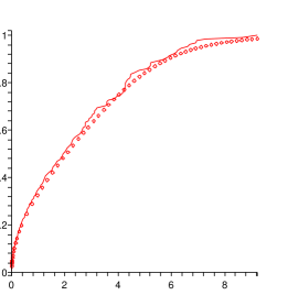
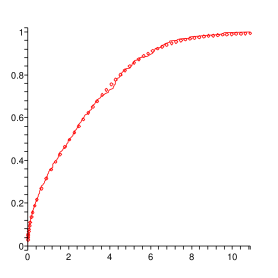
Figure 1. The counting measure $N_{n}$ (solid line) for a particular realisation of the sequence ${\mathbf{s}}$ when $\mu=\mu^{a}$ with $a=8$: (i) $n=128$ and (ii) $n=256$. For comparison, points corresponding to values of the integrated density of states $N$ are also shown.

While the Lyapunov exponent and the density of states are non-random, the measure $\sigma$ is random. We note that $\sigma^{\infty}$ is absolutely continuous whereas, for every $a\in{\mathbb{Z}}_{+}$, almost every realisation of $\sigma$ is singular. Figure 2 shows the approximation

$$\int_{0}^{\lambda}\sigma_{n}(\text{\rm d}\lambda^{\prime})\,,$$

of the integrated measure for particular realisations corresponding to $a=8$ and $a=64$. Here $\sigma_{n}$ is the discrete measure defined by the quadrature formula (1.10), and $n=256$.

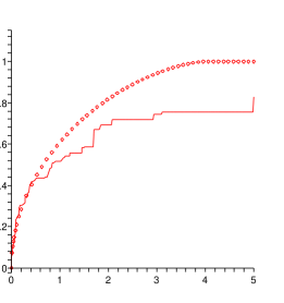
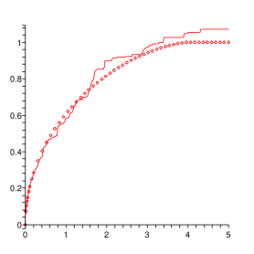
Figure 2. Plot (solid line) of $\int_{0}^{\lambda}\sigma_{n}(\text{\rm d}\lambda^{\prime})$, with $n=256$, corresponding to particular realisations of ${\mathbf{s}}$ when $\mu=\mu^{a}$ where (i) $a=8$ and (ii) $a=64$. For comparison, points corresponding to values of the function $\int_{0}^{\lambda}\sigma^{\infty}(\text{\rm d}\lambda^{\prime})$ are also shown.

Appendix A Proof of proposition 1.1

As mentioned in the introduction, the theory of products of random matrices is a convenient means of deducing the uniqueness of the invariant measure, as well as the positivity of the real part of the complex Lyapunov exponent. For this purpose, we shall have to deal with products of $2\times 2$ matrices with real or complex entries; so, in the following, ${\mathbb{K}}$ will stand for either ${\mathbb{R}}$ or ${\mathbb{C}}$. Set

$$\overline{\mathbb{K}}:={\mathbb{K}}\cup\{\infty\}\,.$$

We define an equivalence relation in the set of nonzero vectors in ${\mathbb{K}}^{2}$ via

$$\begin{pmatrix}u\\ v\end{pmatrix}\sim\begin{pmatrix}u^{\prime}\\ v^{\prime}\end{pmatrix}\quad\text{if $\exists\;w\in{\mathbb{K}}\backslash\{0\}$ such that}\;\begin{pmatrix}u\\ v\end{pmatrix}=w\begin{pmatrix}u^{\prime}\\ v^{\prime}\end{pmatrix}\,.$$

The set of the equivalence classes is called the projective space ${P}({\mathbb{K}}^{2})$. Let

$$\left[\begin{pmatrix}u\\ v\end{pmatrix}\right]\in P\left({\mathbb{K}}^{2}\right)\,.$$

We shall identify this equivalence class with

$$z={\mathcal{P}}\left(\left[\begin{pmatrix}u\\ v\end{pmatrix}\right]\right):=\begin{cases}u/v&\text{if $v\neq 0$}\\ \infty&\text{otherwise}\end{cases}\in\overline{\mathbb{K}}\,.$$

The results of Furstenberg & Kesten (1960) and Furstenberg (1963) concern the typical asymptotic behaviour of the product of independent, identically distributed random elements of some group acting on a compact topological space. In our particular context, the relevant group is the subgroup of $\text{GL}\left(2,{\mathbb{K}}^{2}\right)$ consisting of $2\times 2$ matrices with determinant $\pm 1$, and the topological space is $P\left({\mathbb{K}}^{2}\right)$. The invertible matrices

(A.1) $$\mathcal{A}=\begin{pmatrix}a&b\\ c&d\end{pmatrix}\,,$$

are drawn at random from a distribution which we shall denote by $\tilde{\mu}$. The action of the matrix $\mathcal{A}$ on the projective space can be expressed as

(A.2) $${\mathcal{A}}\cdot\begin{pmatrix}z\\ 1\end{pmatrix}=\begin{pmatrix}{\mathcal{F}}(z)\\ 1\end{pmatrix}\,,$$

where ${\mathcal{F}}:\;\overline{\mathbb{K}}\rightarrow\overline{\mathbb{K}}$ is the linear fractional transformation defined by

(A.3) $${\mathcal{F}}(z)=\mathcal{P}\left(\mathcal{A}\begin{pmatrix}z\\ 1\end{pmatrix}\right)=\begin{cases}\frac{az+b}{cz+d}&\text{if $z\in{\mathbb{K}}$ and $cz+d\neq 0$}\\ \infty&\text{if $c\neq 0$ and $z=-d/c$}\\ a/c&\text{if $z=\infty$ and $c\neq 0$}\\ \infty&\text{if $c=0$ and $z=\infty$}\end{cases}\,.$$

Thus, we have an obvious connection between products

$${\mathcal{U}}_{n}:={\mathcal{A}}_{n}\cdots{\mathcal{A}}_{2}{\mathcal{A}}_{1}$$

of the ${\mathcal{A}}_{n}$ and the Markov chain $\hat{\mathbf{Z}}$ such that

(A.4) $$\hat{Z}_{0}=z,\quad\hat{Z}_{n+1}={\mathcal{F}}_{n}\left(\hat{Z}_{n}\right)\,.$$

Indeed,

(A.5) $$\hat{Z}_{n}={\mathcal{U}}_{n}\cdot\begin{pmatrix}z\\ 1\end{pmatrix}\,.$$

We are interested in the rate of growth of this product as $n\rightarrow\infty$; this is quantified by the number

(A.6) $$\gamma_{\tilde{\mu}}:=\lim_{n\rightarrow\infty}\frac{1}{n}{\mathbb{E}}\left(\ln|{\mathcal{U}}_{n}|\right),$$

where $|\cdot|$ denotes some matrix norm. This limit exists whenever

(A.7) $${\mathbb{E}}(\log^{+}|{\mathcal{A}}|)<\infty\,.$$

In the literature on products of random matrices, the name “Lyapunov exponent” is usually reserved for $\gamma_{\tilde{\mu}}$; as we shall see, it is in fact the real part of the complex Lyapunov exponent introduced earlier.

The following specialisation of Furstenberg’s theorem will be the most useful for our purpose:

Theorem 4.

Let the ${\mathcal{A}}_{n}$ be independent $2\times 2$ random matrices with determinant $\pm 1$ and a common distribution $\tilde{\mu}$. Suppose that there is no measure on $P\left({\mathbb{K}}^{2}\right)$ that is invariant under the action of the smallest subgroup of $\text{\em GL}(2,{\mathbb{K}}^{2})$ generated by the support of $\tilde{\mu}$. Then

1. there exists a unique probability measure $\tilde{\nu}_{\tilde{\mu}}$ on $P\left({\mathbb{K}}^{2}\right)$ that is invariant under the action of matrices in the support of $\tilde{\mu}$.

2. Let $z\in{\mathbb{K}}$. Then, for almost every realisation of the sequence $\{\mathcal{A}_{n}\}_{n\in\mathbb{N}}$,

   $$\lim_{n\rightarrow\infty}\frac{1}{n}\ln\left|{\mathcal{U}}_{n}\cdot\begin{pmatrix}z\\ 1\end{pmatrix}\right|=\gamma_{\tilde{\mu}}\,.$$

3. If condition (A.7) holds, then the number $\gamma_{\tilde{\mu}}$ is strictly positive and is given by the formula

   $$\gamma_{\tilde{\mu}}=\int_{P\left({\mathbb{K}}^{2}\right)}\int_{\text{\em GL}(2,\mathbb{K})}\ln\frac{\left|\mathcal{A}\begin{pmatrix}z\\ 1\end{pmatrix}\right|}{\left|\begin{pmatrix}z\\ 1\end{pmatrix}\right|}\,\tilde{\mu}\left(\text{\em d}\mathcal{A}\right)\,\tilde{\nu}_{\tilde{\mu}}\left(\text{\em d}\begin{pmatrix}z\\ 1\end{pmatrix}\right)\,.$$

Proof.

See Bougerol & Lacroix (1985), Part A, theorem 4.4 on p. 32. The last formula appears in Part A, theorem 3.6 on p. 27 of the same reference. ∎

Corollary A.1.

Let $t\in{\mathbb{C}}\backslash{\mathbb{R}}_{-}$. Let the $s_{n}$ be independent random variables in ${\mathbb{R}}_{+}$ with a common distribution $\mu$ whose support contains at least two points. Set

$${\mathcal{A}}_{n}=\begin{pmatrix}0&1\\ 1&\frac{s_{n}}{\sqrt{t}}\end{pmatrix}\,.$$

Then $\mu$ induces a probability distribution $\tilde{\mu}$ on $\text{\em GL}(2,{\mathbb{C}})$ such that the hypothesis of theorem 4 is fulfilled, and the image $\nu_{\mu}$ of the invariant measure $\tilde{\nu}_{\tilde{\mu}}$ under the map $\mathcal{P}$ is the unique stationary distribution for the Markov chain $\hat{\mathbf{Z}}$. Furthermore, if we also assume that

$$\int_{{\mathbb{R}}_{+}}s^{\varepsilon}\,\mu(\text{\em d}s)<\infty$$

for some $\varepsilon>0$, then we have the formula

$$\gamma_{\tilde{\mu}}=-\int_{\mathbb{C}}\ln|z|\,\nu_{\mu}(\text{\em d}z)\,.$$

Proof.

Same as that of Carmona & Lacroix (1990), corollary IV.4.26. ∎

Corollary A.2.

Let $u_{n}$ be the sequence defined by the recurrence relation (1.16) with $u_{0}\neq 0$. Under the same hypothesis on $\mu$, for every $t\in{\mathbb{C}}\backslash{\mathbb{R}}_{-}$, for almost every realisation of the sequence ${\mathbf{s}}$, we have

$$\lim_{n\rightarrow\infty}\frac{\ln u_{n}}{n}=\Lambda_{\mu}(t)$$

independently of the starting value $u_{0}$.

Proof.

This follows from the equality

$$\frac{\ln u_{n}}{n}=\frac{\ln u_{0}}{n}-\frac{1}{n}\sum_{j=1}^{n}\ln\hat{Z}_{j}\,,$$

the definition of $\Lambda_{\mu}$, and the uniqueness of the stationary measure for the Markov chain $\hat{\mathbf{Z}}$. ∎

For reasons that will become clear when we discuss the nature of the spectrum of the measure $\sigma$, we also need to consider the case where

$$t=-x+\text{\rm i}0\pm\,,\quad x>0\,.$$

In this case,

$${\mathcal{A}}_{n}=\begin{pmatrix}0&1\\ 1&\mp\text{\rm i}\frac{s_{n}}{\sqrt{x}}\end{pmatrix}$$

and so the recurrence defining the Markov chain $\hat{\mathbf{Z}}$ is

$$\hat{Z}_{n+1}=\frac{1}{\hat{Z}_{n}+\mp\text{\rm i}\frac{s_{n+1}}{\sqrt{x}}}\,.$$

Once again, theorem 4 implies the existence of a unique stationary measure $\mu_{\nu}$. We remark that this stationary measure is concentrated on the imaginary axis. Indeed, define $\hat{Y}_{n}$ via

$$\hat{Z}_{n}=\text{\rm i}\hat{Y}_{n}\,.$$

Then

$$\hat{Y}_{n+1}=\frac{-1}{\hat{Y}_{n}+\mp\frac{s_{n+1}}{\sqrt{x}}}\,.$$

The resulting Markov chain $\hat{\mathbf{Y}}=(\hat{Y}_{0}\,,\hat{Y}_{1}\,,\ldots)$ corresponds to the product of the real (Schrödinger) matrices

$$\begin{pmatrix}0&-1\\ 1&\frac{s_{n}}{\sqrt{x}}\end{pmatrix}\,.$$

By applying theorem 4 with ${\mathbb{K}}={\mathbb{R}}$, we deduce that $\hat{\mathbf{Y}}$ has a unique stationary measure supported on ${\mathbb{R}}$. The fact that the measure $\mu_{\nu}$ must be concentrated on the imaginary axis then follows by uniqueness.

Corollary A.3.

Let $u_{n}$ be the sequence defined by the recurrence relation (1.16) with $u_{0}\neq 0$ and $t=-x+\text{\rm i}0\pm$. Under the same hypothesis on $\mu$, for every $x\in{\mathbb{R}}_{+}$, for almost every realisation of the sequence ${\mathbf{s}}$, we have

$$\lim_{n\rightarrow\infty}\frac{\ln u_{n}}{n}=\Lambda_{\mu}(-x+\text{\rm i}0\pm)$$

independently of the starting value $u_{0}$.

Finally, the positivity of $\gamma_{\tilde{\mu}}$, asserted in theorem 4, leads to the

Corollary A.4.

Under the same hypothesis on $\mu$, for every $t\in{\mathbb{C}}\backslash{\mathbb{R}}_{-}$,

$$\text{\rm Re}\left[\Lambda_{\mu}(t)\right]>0\,.$$

Also, for every $x\in{\mathbb{R}}_{+}$,

$$\text{\rm Re}\left[\Lambda_{\mu}(-x+\text{\rm i}0\pm)\right]>0\,.$$

Proof.

Take the real part in equation (1.20) and use corollary A.1 . ∎

The statements made in corollaries A.1-A.4 are of the form:

Let $t$ be fixed, then for almost every realisation of the sequence ${\mathbf{s}}$, etc.

But the proof of proposition 1.1 follows easily from them by a well-known argument based on the use of Fubini’s theorem; see, for instance, Ishii (1973).

Appendix B The complex Lyapunov exponent for the gamma distribution

In this appendix, we derive the formula (1.26) for the complex Lyapunov exponent when $\mu$ is the gamma distribution. For this purpose, it is convenient to adopt the notation used in Marklof et al. (2005); so we set

$$a_{n}:=\frac{s_{n}}{\sqrt{|t|}}\quad\text{and}\quad\alpha:=-\frac{\arg{t}}{2}\in[-\pi/2,\,\pi/2]\,.$$

Then

$$Z=\cfrac{1}{a_{1}\text{\rm e}^{\text{\rm i}\alpha}+\cfrac{1}{a_{2}\text{\rm e}^{\text{\rm i}\alpha}+\cfrac{1}{a_{3}\text{\rm e}^{\text{\rm i}\alpha}+\cdots}}}\,.$$

The random variable $Z$ takes values in the set

$$S_{\alpha}:=\left\{z\in\mathbb{C}\,:\;|\arg z|\leq|\alpha|\right\}\,.$$

In Marklof et al. (2005), we showed that, if the $a_{n}$ are gamma-distributed with parameters $p$ and $s$, then the probability density function of $Z$ is given explicitly by

(B.1) $$f_{\alpha}(z)=\frac{\sin(2|\alpha|)}{\left|2K_{p}\left(2\text{\rm e}^{\text{\rm i}\alpha}/s\right)\right|^{2}}\frac{1}{r^{2}\sin^{2}(\alpha+\theta)}\left[\frac{\sin(\alpha-\theta)}{\sin(\alpha+\theta)}\right]^{p-1}\\ \times\exp\left\{-\frac{\sin(2\alpha)}{s}\left[\frac{1}{r\sin(\alpha-\theta)}+\frac{r}{\sin(\alpha+\theta)}\right]\right\}\,,$$

where $r=|z|$ and $\theta=\arg z$. This is valid for $|\alpha|<\pi/2$— which is all we need for the purpose of calculating the complex Lyapunov exponent, since the cases $\alpha=\pm\pi/2$ may be obtained by letting $\alpha$ tend to the appropriate limit. In Marklof et al. (2005), we derived the formula

$$-\int_{S_{\alpha}}\ln|z|f_{\alpha}(z)\,\text{\rm d}z=\text{\rm Re}\left[\frac{\partial_{p}K_{p}\left(\frac{2}{s}\text{\rm e}^{-\text{\rm i}\alpha}\right)}{K_{p}\left(\frac{2}{s}\text{\rm e}^{-\text{\rm i}\alpha}\right)}\right]\,.$$

So there only remains to show that

(B.2) $$-\int_{S_{\alpha}}\ln\left(\text{\rm e}^{\text{\rm i}\arg z}\right)\,f_{\alpha}(z)\,\text{\rm d}z=\text{\rm i}\text{\rm Im}\left[\frac{\partial_{p}K_{p}\left(\frac{2}{s}\text{\rm e}^{-\text{\rm i}\alpha}\right)}{K_{p}\left(\frac{2}{s}\text{\rm e}^{-\text{\rm i}\alpha}\right)}\right]\,.$$

We shall need the

Lemma B.1.

Let $w$ and $W$ be two complex numbers with positive real part. Then

(B.3) $$K_{p}(w)\,\partial_{p}K_{p}(W)=-\frac{1}{2}\int_{-\infty}^{\infty}\text{\rm e}^{-2pu}\int_{0}^{\infty}\left(u+\ln\frac{2v}{w\text{\rm e}^{u}+W\text{\rm e}^{-u}}\right)\\ \times\exp\left\{-v-\frac{w^{2}+2wW\cosh(2u)+W}{4v}\right\}\,\frac{\text{\rm d}v}{v}\,\text{\rm d}u\,.$$

Proof.

The Bessel function of the second kind has the integral representation (see Watson 1966, §6.22)

$$K_{p}(z)=\frac{1}{2}\int_{-\infty}^{\infty}\text{\rm e}^{-z\cosh x-px}\,\text{\rm d}x\,.$$

Hence

$$K_{p}(W)\partial_{p}K_{p}(w)=-\frac{1}{4}\int_{-\infty}^{\infty}\int_{-\infty}^{\infty}\exp\left\{-W\cosh y-py-w\cosh x-px\right\}\,x\,\text{\rm d}x\text{\rm d}y\,.$$

We make the change of variables

$$x=X+Y\quad\text{and}\quad y=X-Y\,.$$

Then, after some re-arrangement,

(B.4) $$K_{p}(W)\,\partial_{p}K_{p}(w)=-\frac{1}{2}\int_{-\infty}^{\infty}\text{\rm e}^{-2pX}\\ \times\int_{-\infty}^{\infty}\exp\left\{-\text{\rm e}^{Y}\frac{W\text{\rm e}^{-X}+w\text{\rm e}^{X}}{2}-\text{\rm e}^{-Y}\frac{W\text{\rm e}^{X}+w\text{\rm e}^{-X}}{2}\right\}(X+Y)\text{\rm d}Y\text{\rm d}X\,.$$

Make the substitution

$$v=\text{\rm e}^{Y}\frac{W\text{\rm e}^{-X}+w\text{\rm e}^{X}}{2}$$

in the second integral. Then

(B.5) $$K_{p}(W)\,\partial_{p}K_{p}(w)=-\frac{1}{2}\int_{-\infty}^{\infty}\text{\rm e}^{-2pX}\\ \times\int_{-\infty}^{\infty}\exp\left\{-v-\frac{W^{2}+2wW\cosh(2X)+w^{2}}{4v}\right\}\left(X+\ln\frac{2v}{W\text{\rm e}^{-X}+w\text{\rm e}^{X}}\right)\frac{\text{\rm d}v}{v}\text{\rm d}X\,.$$

The desired result follows after we set $X=u$ and take the imaginary part. ∎

Returning to the proof of equation (B.2), let us write

(B.6) $$\text{\rm Im}\int_{S_{\alpha}}\ln\left(\text{\rm e}^{-\text{\rm i}\arg z}\right)\,f_{\alpha}(z)\,\text{\rm d}z=\frac{1}{4\left|K_{p}\left(\frac{2}{s}\text{\rm e}^{-\text{\rm i}\alpha}\right)\right|^{2}}\,{\mathcal{I}}\,,$$

where

(B.7) $${\mathcal{I}}:=\text{\rm Im}\int_{-\alpha}^{\alpha}\int_{0}^{\infty}\ln\left(\text{\rm e}^{-\text{\rm i}\theta}\right)\frac{\sin(2|\alpha|)}{r^{2}\sin^{2}(\alpha+\theta)}\left[\frac{\sin(\alpha-\theta)}{\sin(\alpha+\theta)}\right]^{p-1}\\ \times\exp\left\{-\frac{\sin(2\alpha)}{s}\left[\frac{1}{r\sin(\alpha-\theta)}+\frac{r}{\sin(\alpha+\theta)}\right]\right\}\,\text{\rm d}r\text{\rm d}\theta\,.$$

Replace the variable $r$ by

$$v=\frac{r\sin(2\alpha)}{s\,\sin(\alpha+\theta)}$$

and then the variable $\theta$ by

$$t=\frac{\sin(\alpha-\theta)}{\sin(\alpha+\theta)}\,.$$

A straightforward calculation leads to

(B.8) $${\mathcal{I}}=\text{Im}\int_{0}^{\infty}\ln\left(\frac{\sqrt{t\varphi(t)}}{\text{\rm e}^{\text{\rm i}\alpha}+t\text{\rm e}^{-\text{\rm i}\alpha}}\right)\,t^{p-1}\int_{0}^{\infty}\exp\left\{-v-\frac{4}{s^{2}}\frac{\varphi(t)}{4v}\right\}\frac{\text{\rm d}v}{v}\text{\rm d}t\,,$$

where

$$\varphi(t)=t+\frac{1}{t}+2\cos\alpha\,.$$

Set

$$t=\text{\rm e}^{-2u}\,.$$

Then equation (B.8) becomes

(B.9) $${\mathcal{I}}=-2\,\text{Im}\int_{-\infty}^{\infty}\ln\left(\text{\rm e}^{u+\text{\rm i}\alpha}+\text{\rm e}^{-u-\text{\rm i}\alpha}\right)\,\text{\rm e}^{-2pu}\\ \times\int_{0}^{\infty}\exp\left\{-v-\frac{4}{s^{2}}\frac{\text{\rm e}^{-\text{\rm i}2\alpha}+2\cosh(2u)+\text{\rm e}^{\text{\rm i}2\alpha}}{4v}\right\}\frac{\text{\rm d}v}{v}\text{\rm d}u\,.$$

We use lemma B.3 with $W=\overline{w}=2\text{\rm e}^{-\text{\rm i}\alpha}/s$ to obtain

(B.10) $${\mathcal{I}}=-4\,\text{\rm Im}\left[K_{p}\left(\frac{2}{s}\text{\rm e}^{-\text{\rm i}\alpha}\right)\,\partial_{p}K_{p}\left(\frac{2}{s}\text{\rm e}^{\text{\rm i}\alpha}\right)\right]\\ =4\,\text{\rm Im}\left[K_{p}\left(\frac{2}{s}\text{\rm e}^{\text{\rm i}\alpha}\right)\,\partial_{p}K_{p}\left(\frac{2}{s}\text{\rm e}^{-\text{\rm i}\alpha}\right)\right]\,.$$

The result is then an immediate consequence of equation (B.6).

Appendix C A result of Goldsheid & Khoruzhenko (2005)

In order to deduce the existence of the integrated density of states from proposition 2.1, we shall need some technical results contained in Goldsheid & Khoruzhenko (2005).

Let $\{\mathscr{A}_{n}\}_{n\in{\mathbb{Z}}_{+}}$ be a deterministic sequence of square matrices of increasing dimension $n$, and let

$$p_{n}(z)=\frac{1}{n}\ln\left|\text{det}\left(\mathscr{A}_{n}-z\mathscr{I}_{n}\right)\right|=\int_{\mathbb{C}}\ln\left|w-z\right|\kappa_{n}(\text{\rm d}w)\,,$$

where $\mathscr{I}_{n}$ is the $n\times n$ identity matrix and

$$\kappa_{n}=\frac{1}{2\pi}\Delta p_{n}$$

is the normalised eigenvalue counting measure of $\mathscr{A}_{n}$. Define

(C.1) $$\tau_{R}:=\overline{\lim_{n\rightarrow\infty}}\int_{|w|\geq R}\ln|w|\,\kappa_{n}(\text{\rm d}w)\,,\quad R\geq 1\,.$$

Proposition C.1.

Assume that there is a function $p\,:\;{\mathbb{C}}\rightarrow[-\infty,\,\infty)$ such that

$$p_{n}(z)\xrightarrow[n\rightarrow\infty]{}p(z)\quad\text{for Lebesgue-almost every $z\in{\mathbb{C}}$}\,.$$

If $\tau_{1}<\infty$, then

1. $p$ is locally integrable.

2. The measure

   $$\kappa:=\frac{1}{2\pi}\Delta p$$

   is a probability measure.

3. We have

   $$\int_{|w|\geq 1}\ln|w|\,\kappa(\text{\em d}w)\leq\tau_{1}<\infty$$

   and the sequence $\{\kappa_{n}\}_{n\in{\mathbb{Z}}_{+}}$ converges weakly to $\kappa$.

Proof.

See Goldsheid & Khoruzhenko (2005), proposition 1.3. ∎

To apply this result in our context, we set $\mathscr{A}_{n}=\mathscr{J}_{n}$. Proposition 2.1 then takes care of the first assumption. There remains to show the finiteness of $\tau_{1}$. Goldsheid & Khoruzhenko remark that the following inequalities hold:

$$\tau_{1}\leq\overline{\lim_{n\rightarrow\infty}}\frac{1}{2n}\text{tr}\ln\left(\mathscr{I}_{n}+\mathscr{J}_{n}\mathscr{J}_{n}^{\ast}\right)$$

and

(C.2) $$\frac{1}{n}\text{tr}\ln\left(\mathscr{I}_{n}+\mathscr{J}_{n}\mathscr{J}_{n}^{\ast}\right)\leq\frac{\alpha}{n}\sum_{j=0}^{n-1}\ln\left(1+\beta|{\mathbf{r}}_{j}|^{2}\right)\,,$$

for some positive constants $\alpha$ and $\beta$ independent of $n$ and ${\mathbf{r}}_{j}$, the $j$th row of $\mathscr{J}_{n}$. Now,

(C.3) $$|{\mathbf{r}}_{n}|^{2}=h_{n-1}^{2}+v_{n}^{2}+h_{n}^{2}\\ =\frac{1}{s_{2n+2}^{2}s_{2n+1}s_{2n+3}}+\frac{1}{s_{2n+1}^{2}}\left(\frac{1}{s_{2n+2}}+\frac{1}{s_{2n+3}}\right)^{2}+\frac{1}{s_{2n}^{2}s_{2n-1}s_{2n+1}}$$

and, so by repeated use of the elementary inequality

$$ab\leq\frac{1}{2}\left(a^{2}+b^{2}\right)\,,$$

we obtain readily

$$|{\mathbf{r}}_{n}|^{2}\leq\frac{5}{2}\left(\frac{1}{s_{2n-1}^{4}}+\cdots+\frac{1}{s_{2n+3}^{4}}\right)\,.$$

It follows that

(C.4) $$\ln\left(1+\beta|{\mathbf{r}}_{n}|^{2}\right)\leq\ln\left(1+\frac{25}{2}\beta\max\left\{s_{2n-1}^{-4},\,\ldots,\,s_{2n+3}^{-4}\right\}\right)\\ \leq\ln\left(1+\frac{25}{2}\beta s_{2n-1}^{-4}\right)+\cdots+\ln\left(1+\frac{25}{2}\beta s_{2n+3}^{-4}\right)\,.$$

We deduce from the ergodic theorem that the right-hand side of equation (C.2) is bounded independently of $n$ provided that

$$\int_{{\mathbb{R}}_{+}}\ln\left(1+\frac{25}{2}\frac{\beta}{s^{4}}\right)\,\mu(\text{\rm d}s)<\infty\,.$$

This last inequality follows easily from our hypothesis that

$$\int_{{\mathbb{R}}_{+}}\left|\ln s\right|\,\mu(\text{\rm d}s)<\infty\quad\text{and}\quad\int_{{\mathbb{R}}_{+}}s^{\varepsilon}\,\mu(\text{\rm d}s)<\infty\,.$$

References

[1]
[2]Abramowitz, M. & Stegun, I. A. 1964 Handbook of Mathematical Functions. Dover.
[3]
[4]Akhiezer, N. I. 1961 The Classical Moment Problem and Related Problems in Analysis.
Fizmatgiz. (Transl. Oliver and Boyd, 1965).
[5]
[6]Bender, C. & Orszag, S. A. 1978 Advanced
Mathematical Methods for Scientists and Engineers.
McGraw–Hill.
[7]
[8]Bougerol, P. & Lacroix, J. 1985 Products of
Random Matrices with Applications to Schrödinger Operators.
Birkhäuser.
[9]
[10]Breiman, L. 1960 The strong law of large numbers for a class of Markov chains.
Ann. Math. Stat.31, 801-803.
[11]
[12]Carmona, R. & Lacroix, J. 1990 Spectral Theory of Random Schrödinger
operators. Birkhäuser.
[13]
[14]Csordas, G., Hilden, H. & Pitcher, T. 1973 Random functions in .
Z. Wahrsch. Verw. Gebiete26,
325-334.
[15]
[16]Diaconis, P. & Freedman, D. 1999 Iterated random functions, SIAM Rev.41, 45-76.
[17]
[18]Dyson, F. J. 1953 The dynamics of a disordered linear chain. Phys. Rev.92,
1331-1338.
[19]
[20]Foster, S. & Pitcher, T. 1974 Convergence properties of random -fractions.
Z. Wahrsch. Verw. Gebiete29,
323-330.
[21]
[22]Furstenberg, H. 1963 Non commuting random products. Trans. Amer. Math. Soc.108, 377-428.
[23]
[24]Furstenberg, H. & Kesten, H. 1960 Products of random matrices.
Ann. Math. Statist.31, 377-428.
[25]
[26]Geronimo, J. S. 1993 Polynomials orthogonal on the unit circle with random recurrence
coefficients. In Methods of approximation theory in complex analysis and mathematical physics (Leningrad, 1991). Springer Lecture Notes in Mathematics, no. 1550, pp. 43-61.
[27]
[28]Goldsheid, I. & Khoruzhenko, B. 2005 The Thouless formula for random non-hermitian
Jacobi matrices. Israël J. Math.148, 331-346.
[29]
[30]Ishii, K. 1973 Localization of eigenstates and transport phenomena in the one-dimensional
disordered system. Suppl. Prog. Theor. Phys.53, 77-138.
[31]
[32]Letac, G. & Seshadri, V. 1983 A characterisation of the
generalised inverse gaussian distribution by continued fractions.
Z. Wahrsch. Verw. Gebiete62, 485-489.
[33]
[34]Luck, J. M. 1992 Systèmes désordonnés unidimensionnels. Alea.
[35]
[36]Mannion, D. 1993 Products of matrices. Ann. Appl. Probab.3,
1189-1218.
[37]
[38]Marklof, J., Tourigny, Y. & and Wołowski, L. 2005 Explicit invariant measures for products of random matrices. To
appear in Trans. Amer. Math. Soc..
[39]
[40]Meyn, P. & Tweedie, R. 1993 Markov Chains and Stochastic Stability, Springer-Verlag.
[41]
[42]Nikishin, E. M. & Sorokin, V. N. 1988 Rational Approximation and Orthogonality.
Nauk. (English Transl. American Mathematical Society, 1991.)
[43]
[44]Pastur, L. & Figotin, A. 1992 Spectra of Random and Almost-Periodic Operators.
Springer-Verlag.
[45]
[46]Schmidt, H. 1957 Disordered one-dimensional crystals. Phys. Rev.105, 425-441.
[47]
[48]Simon, B. 1998 The classical moment problem as a self-adjoint finite
difference operator. Adv. Math.117, 82-203.
[49]
[50]Stieltjes, T. J. 1894 Recherches sur les fractions
continues. Ann. Fac. Sci. Toulouse8, 1-122.
[51]
[52]Wall, H. S. 1948 Analytic theory of continued fractions. Van Nostrand.
[53]
[54]Watson, G. N. 1966 A treatise on the theory of Bessel functions. Cambridge University Press.
[55]
[56]Yoshioka, Y. 1973 On the singularity of the spectral measures of a semi-infinite
random system. Proc. Japan Acad.49, 665-668.