Troubleshooting Time-Dependent Density-Functional Theory for Photochemical Applications: Oxirane

Abstract

The development of analytic-gradient methodology for excited states within conventional time-dependent density-functional theory (TDDFT) would seem to offer a relatively inexpensive alternative to better established quantum-chemical approaches for the modeling of photochemical reactions. However, even though TDDFT is formally exact, practical calculations involve the use of approximate functionals, in particular the TDDFT adiabatic approximation, whose use in photochemical applications must be further validated. Here, we investigate the prototypical case of the symmetric CC ring opening of oxirane. We demonstrate by direct comparison with the results of high-quality quantum Monte Carlo calculations that, far from being an approximation on TDDFT, the Tamm-Dancoff approximation (TDA) is a practical necessity for avoiding triplet instabilities and singlet near instabilities, thus helping maintain energetically reasonable excited-state potential energy surfaces during bond breaking. Other difficulties one would encounter in modeling oxirane photodynamics are pointed out but none of these is likely to prevent a qualitatively correct TDDFT/TDA description of photochemistry in this prototypical molecule.

I Introduction

A complete understanding of photochemistry often requires photodynamics calculations since photochemical reactions may have excess energy and do not follow the lowest energy pathway, and since dynamic, as much as energetic, considerations often govern how a reaction jumps from one electronic potential energy surface (PES) to another. Unfortunately, full photodynamics calculations are prohibitively expensive for all but the smallest molecules unless simplifying approximations are made. One such approximation is to adopt a Tully-type mixed quantum/classical surface-hopping (SH) trajectory approach TP71 ; T90 where the electrons are described quantum mechanically and the nuclei classically. Then, since the quantum part of the calculation remains the computational bottleneck, further simplifications are required for an efficient electronic structure computation of the photochemical dynamics.

Time-dependent density-functional theory (TDDFT) MUN+06 represents a promising and relatively inexpensive alternative DM02 to accurate but more costly quantum chemical approaches for on-the-fly calculations of excitation energies. TDDFT methods for excited-state dynamics are not yet a standard part of the computational chemistry repertory but are coming on line. In particular, the basic methodology for the computation of analytic gradients has now been implemented in a number of codes VA99 ; VA00 ; FA02 ; RF05 ; H03 ; DK05 and important practical progress is being made on the problem of calculating SH integrals within TDDFT CM00 ; B02 ; CDP05 ; M06 ; HCP06 ; TTR07 . Indeed first applications of mixed TDDFT/classical SH dynamics are being reported CDP05 ; HCP06 ; TTR07 . Problems in this new technology can be expected and modifications in the basic TDDFT methods will be necessary to enlarge the class of its potential applications. In particular, practical TDDFT calculations employ approximate functionals whose performance in describing photochemical problems requires careful validation.

Few applications of TDDFT to problems relevant to photochemistry can be found in the literature DKZ01a ; DKZ01b ; DKSZ02 ; SDK+02 ; OGB02 ; CSM+06 and the few attempts made to assess the value of TDDFT for photochemical applications report either encouraging CCS98 ; FMO04 ; BGDF06 or discouraging results BM00 ; CTR00 ; RCT04 ; WGB+04 ; LQM06 . The fundamental reasons for these descrepencies stem from the fact that conventional TDDFT has several problems which may or may not be fatal for modeling a given photochemical reaction. The main difficulties encountered in conventional TDDFT include the underestimation of the ionization threshold CCS98 , the underestimation of charge transfer excitations TAH+99 ; CGG+00 ; DWH03 , and the lack of explicit two- and higher-electron excitations C95 ; MZCB04 ; CZMB04 ; C05 . Still other difficulties are discussed in pertinant reviews C01 ; MBA+01 ; ORR02 ; D03 ; MWB03 ; SM05 ; MUN+06 .

To help TDDFT become a reliable tool for modeling photochemistry, we must first obtain a clear idea of what are its most severe problems. It is the objective of this article to identify the most critical points where improvement needs to be made, at least for one prototypical molecule and one type of reaction path. The reaction chosen for our study is the photochemical ring opening of oxirane. The photochemistry of oxirane and of oxirane derivatives has been much studied both theoretically and experimentally (Appendix A). It is a text-book molecule used to discuss orbital control of stereochemistry in the context of electrocyclic ring opening. Textbook discussions usually focus on CC ring opening (see e.g. Ref. MB90 pp. 258-260) but a discussion of CO ring opening may also be found (Ref. MB90 pp. 408-411). At first glance, this would seem to be a particularly good test case for TDDFT. That is, oxirane is a simple molecule with a relatively simple photochemistry where TDDFT should work and, if not, where its failures will be particularly easy to analyze. In this paper, we will focus on the symmetric ring opening of this molecule even though the photochemical ring opening does not follow a symmetric pathway. The reason for our choice is the usual reason symmetry , namely that the use of symmetry greatly facilitates analysis and hence the construction of and comparison with highly accurate quantum Monte Carlo results. A mixed quantum/classical SH trajectory study of asymmetric ring opening will be reported elsewhere T07 .

In the next section, we give a brief review of DFT and of TDDFT. In sec. III, we review the formalism behind the more exact theory against which we will be comparing our TDDFT results. Computational details are given in Sec. IV. Section V reports our results and discussion and Sec. VI summarizes.

II (Time-Dependent) Density-Functional Theory

The (TD)DFT PES for the $I$th excited state is calculated at each nuclear configuration by adding the $I$th TDDFT excitation energy to the DFT ground state energy, so $E_{I}=E_{0}+\omega_{I}$. [Hartree atomic units ($\hbar=m=e=1$) are used throughout the paper.] Even though the use of parentheses in the expression (TD)DFT better emphasizes the hybrid DFT + TDDFT nature of the calculation, we will usually follow the common practice of simply refering to TDDFT PESs. The purpose of this section is to review those aspects of TDDFT most necessary for understanding the rest of the paper.

The hybrid DFT + TDDFT nature of (TD)DFT calculations indicates that problems with the ground state PES can easily become problems for the excited-state PESs. Thus it is important to begin with a few words about the ground-state problem. The simplest methods for treating the ground state are the Hartree-Fock (HF) method and the Kohn-Sham formulation of DFT. In recent years, the use of hybrid functionals has permitted the two energy expressions to be written in the same well-known form,

$$E^{\text{hybrid}}_{xc}=E^{\text{GGA}}_{xc}+c_{x}(E^{\text{HF}}_{x}-E^{\text{GGA}}_{x})$$ (1)

where $E^{\text{HF}}_{x}$ is the HF exchange energy and $E^{\text{GGA}}_{x}$ and $E^{\text{GGA}}_{xc}$ are generalized gradient approximation (GGA) exchange (x) and exchange-correlation (xc) energies. The coefficient $c_{x}$ controls the amount of Hartree-Fock exchange, being unity for Hartree-Fock, zero for pure DFT, and fractional (typically around 0.25 PEB96 ) for hybrid functionals. For more information about DFT, we refer the reader to Refs. PY89 ; DG90 ; KH00 .

Time-dependent density-functional theory offers a rigorous approach to calculating excitation energies. Unlike time-dependent Hartree-Fock (TDHF), TDDFT is formally exact. Consequently, although approximate exchange-correlation functionals must be used in practice, we can hope that good approximations will lead to better results than those obtained from TDHF which completely lacks correlation effects. In practice, the use of hybrid functionals means that TDDFT contains TDHF as a particular choice of functional (i.e., the exchange-only hybrid functional with $c_{x}=1$).

The most common implementation of TDDFT is via a Kohn-Sham formalism using the so-called adiabatic approximation which assumes that the self-consistent field responds instantaneously and without memory to any temporal change in the charge density. This allows the time-dependent exchange-correlation action quantity in TDDFT to be replaced with the more familiar exchange-correlation energy from conventional TDDFT. Excitations may be obtained from the linear response formulation of TDDFT (LR-TDDFT). A key quantity in LR-TDDFT is the exchange-correlation kernel,

$$f_{xc}^{\sigma,\tau}({\bf r},{\bf r}^{\prime})=\frac{\delta^{2}E_{xc}[\rho_{\uparrow},\rho_{\downarrow}]}{\delta\rho_{\sigma}({\bf r})\delta\rho_{\tau}({\bf r}^{\prime})}\,,$$ (2)

which, along with the Hartree kernel, $f_{H}^{\sigma,\tau}({\bf r},{\bf r}^{\prime})=1/\left|{\bf r}-{\bf r}^{\prime}\right|$, and the Hartree-Fock exchange kernel (whose integrals can be written in terms of the Hartree kernel) determines the linear response of the Kohn-Sham self-consistent field in the adiabatic approximation. In Casida’s formulation C95 , the excitation energies are obtained by solving a random phase approximation (RPA)-like pseudo-eigenvalue equation,

$$\left[\begin{array}[]{cc}{\bf A}&{\bf B}\\ {\bf B}&{\bf A}\end{array}\right]\left(\begin{array}[]{c}\vec{X}_{I}\\ \vec{Y}_{I}\end{array}\right)=\omega_{I}\left[\begin{array}[]{cc}+{\bf 1}&{\bf 0}\\ {\bf 0}&-{\bf 1}\end{array}\right]\left(\begin{array}[]{c}\vec{X}_{I}\\ \vec{Y}_{I}\end{array}\right)\,,$$ (3)

where the matrices ${\bf A}$ and ${\bf B}$ are defined by,

$$A_{ia\sigma,jb\tau} = \delta_{i,j}\delta_{a,b}\delta_{\sigma,\tau}\left(\epsilon_{a\sigma}-\epsilon_{i\sigma}\right)+\left(ia|f_{H}|bj\right)+\left(ia|f_{xc}^{\sigma,\tau}|bj\right)$$

$$- c_{x}\delta_{\sigma,\tau}\left[\left(ij|f_{H}|ba\right)+\left(ia|f_{x}^{\sigma,\sigma}|bj\right)\right]$$

$$B_{ia\sigma,bj\tau} = \left(ia|f_{H}|jb\right)+\left(ia|f_{xc}^{\sigma,\tau}|jb\right)$$ (4)

$$- c_{x}\delta_{\sigma,\tau}\left[\left(ib|f_{H}|ja\right)+\left(ia|f_{x}^{\sigma,\sigma}|jb\right)\right]\,,$$

and the integrals are in Mulliken charge cloud notation,

$$\left(pq|f|rs\right)=\int\int\psi_{p}^{*}({\bf r})\psi_{q}({\bf r})f({\bf r},{\bf r}^{\prime})\psi_{r}^{*}({\bf r}^{\prime})\psi_{s}({\bf r}^{\prime})\,d{\bf r}d{\bf r}^{\prime}\,.$$ (5)

It is to be emphasized that the TDDFT adiabatic approximation includes only dressed one-electron excitations C95 ; C05 . This is particularly easy to see in the context of the Tamm-Dancoff approximation (TDA) to Eq. (3) whose TDDFT variant is usually attributed to Hirata and Head-Gordon HH99 . The TDA simply consists of neglecting the ${\bf B}$ matrices to obtain, ${\bf A}\vec{X}_{I}=\omega_{I}\vec{X}_{I}$. The number of possible solutions to this equation is the dimensionality of ${\bf A}$ which is just the number of single excitations. In fact, the LR-TDHF TDA (exchange-only hybrid functional with $c_{x}=1$) is simply the well-known configuration interaction singles (CIS) method.

An issue of great importance in the context of the present work is triplet instabilities. These have been first analyzed by Bauernschmitt and Ahlrichs BA96 in the context of DFT, but the explicit association with LR-TDDFT excitation energies was made later CGG+00 ; C01 . Following Ref. C01 , we suppose that the ground-state DFT calculation has been performed using a same-orbitals-for-different-spin (SODS) ansatz and we now wish to test to see if releasing the SODS restriction to give a different-orbitals-for-different-spin (DODS) solution will lower the energy. To do so we consider an arbitary unitary tranformation of the orbitals,

$$\psi_{r\sigma}^{\lambda}({\bf r})=\exp\left[i\lambda\left(\hat{R}+i\hat{I}\right)\right]\psi_{r\sigma}({\bf r})\,.$$ (6)

where $\hat{R}$ and $\hat{I}$ are real operators. The corresponding energy expression is,

$$E_{\lambda}=E_{0}+\lambda^{2}\left[\vec{R}^{\dagger}\left({\bf A}-{\bf B}\right)\vec{R}+\vec{I}^{\dagger}\left({\bf A}+{\bf B}\right)\vec{I}\right]+{\cal O}(\lambda^{3})\,,$$ (7)

where matrix elements of the $\hat{R}$ and $\hat{I}$ operators have been arranged in column vectors and the ${\cal O}(\lambda)$ term disappears because the energy has already been minimized before considering symmetry-breaking. The presence of the terms $({\bf A}\pm{\bf B})$ shows the connection with the pseudoeigenvalue problem (3) which can be rewritten as the eigenvalue problem,

$$\left({\bf A}+{\bf B}\right)\left({\bf A}-{\bf B}\right)\vec{Z}_{I}=\omega_{I}^{2}\vec{Z}_{I}\,,$$ (8)

where $\vec{Z}_{I}=\vec{X}_{I}-\vec{Y}_{I}$. It is an easy consequence of Eq. (4) that the matrix $\left({\bf A}-{\bf B}\right)$ is always positive definite for pure functionals ($c_{x}=0$), as long as the aufbau principle is obeyed. However $\left({\bf A}+{\bf B}\right)$ may have negative eigenvalues. In that case, the energy $E_{\lambda}$ will fall below $E_{0}$ for some value of $\vec{I}$, indicating a lower symmetry-broken solution. At the same time, this will correspond to a negative value of $\omega_{I}^{2}$ (i.e., an imaginary value of $\omega_{I}$.) A further analysis shows the corresponding eigenvector corresponds to a triplet excitation, hence the term “triplet instability” for describing this phenomenon. In principle, when hybrid functionals are used, singlet instabilities are also possible.

Thus imaginary excitation energies in LR-TDDFT are an indication that something is wrong in the description of the ground state whose time-dependent response is being used to obtain those excitation energies. As pointed out in Refs. CGG+00 and CIC06 , the TDA actually acts to decouple the excited-state problem from the ground-state problem so that TDA excitations may actually be better than full LR-TDDFT ones. Typically, full and TDA LR-TDDFT excitation energies are close near a molecule’s equilibrium geometry, where a single-determinantal wave function is a reasonable first approximation and begin to differ as the single-determinantal description breaks down.

Interestingly, there is a very simple argument against symmetry breaking in exact DFT for molecules with a nondegenerate ground state. Since the exact ground-state wave function of these molecules is a singlet belonging to the totally symmetric representation and so with the same symmetry as the molecule, the spin-up and spin-down charge densities will be equal and also have the same symmetry as the molecule. It follows that the same must hold for the spin-up and spin-down components of the exact exchange-correlation potential. Since the potentials are the same, then the molecular orbitals must also be the same for different spins. Thus, no symmetry breaking is expected in exact DFT for molecules with a nondegenerate ground state. Note however that the functional is still dependent on spin so that the spin kernels $f_{xc}^{\uparrow,\uparrow}({\bf r},{\bf r}^{\prime})$ and $f_{xc}^{\uparrow,\downarrow}({\bf r},{\bf r}^{\prime})$ are different.

The interested reader will find additional information about TDDFT in the recent book of Ref. MUN+06 .

III Quantum Monte Carlo

The quality of our (TD)DFT calculations is judged against highly accurate quantum Monte Carlo (QMC) results. For each state of interest, the QMC results are obtained in a three step procedure. First, a conventional complete active space (CAS) self-consistent field (SCF) calculation is performed. The resultant CASSCF wave function is then reoptimized in the presence of a Jastrow factor to include dynamical correlation and used in a variational Monte Carlo (VMC) calculation. Finally, the VMC result is further improved via diffusion Monte Carlo (DMC).

To properly describe a reaction involving bond breaking, it is necessary to adopt a multi-determinantal description of the wave function. In the CASSCF method, a set of active orbitals is selected, whose occupancy is allowed to vary, while all other orbitals are fixed as either doubly occupied or unoccupied. In a CASSCF($n$,$m$) calculation, $n$ electrons are distributed among an active space of $m$ orbitals and all possible resulting space- and spin-symmetry-adapted configuration state functions (CSFs) are constructed. The final CASSCF($n$,$m$) wave function consists of a linear combination of these CSFs, like in a full configuration interaction (CI) calculation for $n$ electrons in $m$ orbitals, except that also the orbitals are now optimized to minimize the total energy. In the present article, we consider 4 electrons in an active space of 6 orbitals which represents the minimal active space for a proper description of all 9 states of interest.

When several states of the same symmetry are requested, there is a danger in optimizing the higher states that their energy is lowered enough to approach and mix with lower states, thus giving an unbalanced description of excitation energies. A well-established solution to this problem is the use of a state averaged (SA) CASSCF approach where the weighted average of the energies of the states under consideration is optimized WM81 ; HJO00 . The wave functions of the different states depend on their individual sets of CI coefficients using a common set of orbitals. Orthogonality is ensured via the CI coefficients and a generalized variational theorem applies. Obviously, the SA-CASSCF energy of the lowest state will be higher than the CASSCF energy obtained without SA. In the present work, we need to apply the SA procedure only for the $2^{1}A_{1}$ state in the $C_{2v}$ ring opening. Although the CASSCF and SA-CASSCF $1^{1}A_{1}$ energies are found to be really very close, we calculate the $2^{1}A_{1}$ energy as $E_{\text{CAS}}(1^{1}A_{1})+\left[E_{\text{CAS}}^{\text{SA}}(2^{1}A_{1})-E_{\text{CAS}}^{\text{SA}}(1^{1}A_{1})\right]$. A similar procedure is used in the case of the corresponding QMC calculations.

QMC methods FMNR01 offer an efficient alternative to conventional highly-correlated ab initio methods to go beyond CASSCF and provide an accurate description of both dynamical and static electronic correlation. The key ingredient which determines the quality of a QMC calculation is the many-body trial wave function which, in the present work, is chosen of the Jastrow-Slater type with the particular form,

$$\Psi^{\text{VMC}}_{I}=\Psi^{\text{CAS}}_{I}\prod_{A,i,j}{\cal J}(r_{ij},r_{iA},r_{jA})\,,$$ (9)

where $r_{ij}$ denotes the distance between electrons $i$ and $j$, and $r_{iA}$ the distance of electron $i$ from nucleus $A$. We use here a Jastrow factor ${\cal J}$ which correlates pairs of electrons and each electron separately with a nucleus, and employ different Jastrow factors to describe the correlation with different atom types. The determinantal component consists of a CAS expansion, $\Psi^{\text{CAS}}_{I}$, and includes all possible CSFs obtained by placing 4 electrons in the active space of 6 orbitals as explained above.

All parameters in both the Jastrow and the determinantal component of the wave function are optimized by minimizing the energy. Since the optimal orbitals and expansion coefficients in $\Psi^{\text{CAS}}_{I}$ may differ from the CASSCF values obtained in the absence of the Jastrow factor ${\cal J}$, it is important to reoptimize them in the presence of the Jastrow component.

For a wave function corresponding to the lowest state of a given symmetry, we follow the energy-minimization approach of Ref. UTFSH07 . If the excited state is not the lowest in its symmetry, we obtain the Jastrow and orbitals parameters which minimize the average energy over the state of interest and the lower states, while the linear coefficients in the CSF expansion ensure that orthogonality is preserved among the states F07 . Therefore, the wave functions resulting from the state-average optimization will share the same Jastrow parameters and the same set of orbitals but have different linear coefficients. This scheme represents a generalization of the approach of Ref. SF04 where only the orbitals were optimized and orthogonality was only approximately preserved. The present approach is therefore superior to the one of Ref. SF04 , which was however already giving excellent results when tested on several singlet states of ethylene and a series of prototypical photosensitive molecules SF04 ; SBF04 . We note that, when a CAS expansion is used in the absence of the Jastrow component, the method is analogous to the CASSCF technique for the lowest state of a given symmetry, and to a SA-CASSCF approach if the excited state is not the lowest in its symmetry.

The trial wave function is then used in diffusion Monte Carlo (DMC), which produces the best energy within the fixed-node approximation [i.e., the lowest-energy state with the same zeros (nodes) as the trial wave function]. All QMC results presented are from DMC calculations.

IV Computational Details

IV.1 SCF and TD Details

Calculations were carried out with two different computer programs, namely Gaussian 03 Gaussian and a development version of deMon2k deMon2K . We use the two programs in a complementary fashion as they differ in ways which are important for this work. In particular, Gaussian can carry out HF calculations while deMon2k has no Hartree-Fock exchange. Similarly, Gaussian can carry out time-dependent HF (TDHF) and configuration interaction singles (CIS) calculations which are not implemented in deMon2k. In contrast, the Tamm-Dancoff approximation (TDA) for TDDFT may only be performed with deMon2k. The present version of deMon2k is limited to the local density approximation for the exchange-correlation TDDFT kernel, while the kernel is more general in Gaussian. Finally, Gaussian makes automatic use of symmetry and prints out the irreducible representation for each molecular orbital. The particular version of deMon2k used in the present work does not have this feature so we rely on comparison with the output of Gaussian calculations for this aspect of our analysis.

All Gaussian results reported here are calculated with the extensive 6-311++G**(2d,2p) basis set KBSP80 ; CCS83 . All calculations used default convergence criteria. The DFT calculations used the default grid for the exchange-correlation integrals.

The same basis set is used for deMon2k calculations as in the Gaussian calculations. The GEN-A3* density-fitting basis set is used and density-fitting is carried out without imposing the charge conservation constraint. The SCF convergence cutoff is set at $10^{-7}$. We always use the FIXED FINE option for the grid. Our implementation of TDDFT in deMon2k is described in Ref. IFP+05 .

We use two different density functionals, the local density approximation (LDA) in the parameterization of Vosko, Wilk, and Nusair VWN80 (referred to as SVWN5 in the Gaussian input), and the popular B3LYP hybrid functional B3LYP . The corresponding TDDFT calculations are referred to as TDLDA and TDB3LYP respectively.

IV.2 CAS Details

All CASSCF calculations are performed with the program GAMESS(US) Gamess . In all SA-CASSCF calculations, equal weights are employed for the two states.

We use scalar-relativistic energy-consistent Hartree-Fock pseudopotentials BFD07 where the carbon and oxygen 1$s$ electrons are replaced by a non-singular $s$-non-local pseudopotential and the hydrogen potential is softened by removing the Coulomb divergence. We employ the Gaussian basis sets BFD07 constructed for these pseudopotentials and augment them with diffuse functions. All calculations are performed with the cc-TZV contracted (11$s$11$p$1$d$)/[3$s$3$p$1$d$] basis for carbon and oxygen, augmented with two additional diffuse $s$ and $p$ functions with exponents 0.04402 and 0.03569 for carbon, and 0.07376 and 0.05974 for oxygen. The $d$ polarization functions for carbon and oxygen are taken from the cc-DZV set. For hydrogen, the cc-DZV contracted (10$s$9$p$)/[2$s$1$p$] basis is augmented with one $s$ diffuse function with exponent 0.02974.

IV.3 QMC Details

The program package CHAMP Champ is used for the QMC calculations. We employ the same pseudopotentials and basis sets as in the CASSCF calculations (see Sec. IV.2).

Different Jastrow factors are used to describe the correlation with a hydrogen, an oxygen and a carbon atom. For each atom type, the Jastrow factor consists of an exponential of the sum of two fifth-order polynomials of the electron-nuclear and the electron-electron distances, respectively FU96 . The parameters in the Jastrow factor and in the determinantal component of the wave function are simultaneously optimized by energy minimization following the scheme of Ref. UTFSH07 , where we employ the simple choice $\xi=1$. For the excited states with the same symmetry as the ground state, the ground- and excited-state wave functions are optimized in a state-average manner with equal weights for both states F07 . An imaginary time step of 0.075 H^-1 is used in the DMC calculations.

V Results

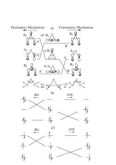
Figure 1: a) Woodward-Hoffmann orbital correlation scheme. Symmetry labels are for the $C_{2v}$ point group in the case of reactants and products, for the $C_{s}$ point group along the disrotatory pathway, and for the $C_{2}$ point group along the conrotatory pathway. b) Thermal ring opening. c) Photochemical ring opening. Symmetry labels depend upon the labels of the $x$, $y$, and $z$ coordinates. In this article, the COC ring lies in the $(y,z)$-plane and the $z$-axis coincides with the $C_{2}$ axis, in agreement with the IUPAC conventionM55 .

The Woodward-Hoffmann (WH) rules for orbital control of symmetry in electrocyclic reactions were an important motivation in the 1970s and 1980s to seek stereospecific photochemical ring-opening reactions of oxiranes H71b ; GP76 ; L76 ; H77 ; HRS+80 ; P87 . Since some oxiranes (notably diphenyl oxirane) do appear to follow the WH rules for thermal and photochemical ring opening, the WH rules might seem like the obvious place to begin our study of symmetric ring opening pathways in oxirane. This is somewhat counterbalanced by the fact that oxirane itself is an exception to the WH rules for photochemical ring opening and by the fact that it is now clear that the WH rules do not apply nearly as well to photochemical as to thermal reactions (Appendix A). Nevertheless, we will take the WH model as a first approximation for understanding and begin by describing the model for the particular case of oxirane.

Many models at the time that Woodward and Hoffmann developed their theory WH65a ; WH65b ; WH69 were based upon simple Hückel-like $\pi$-electron models, so, not surprisingly, the historical WH model for oxirane uses a three-orbital model consisting of one $p$-orbital on each of the oxygen and two carbon atoms. (See Fig. 1.) Elementary chemical reasoning predicts that the closed cycle should form three molecular orbitals, $\sigma$, $n$, $\sigma^{*}$, in increasing order of energy. Similarly the open structure has the “particle-in-a-box” orbitals familiar from simple Hückel theory. Woodward and Hoffmann observed that a reflection plane ($\sigma$) of symmetry is preserved along the disrotatory reaction pathway while a $C_{2}$ rotation symmetry element is preserved along the conrotatory reaction pathway. This observation allows the reactant-product molecular orbital correlation diagram to be completed by using the fact that the symmetry representation of each orbital is preserved within the relevant symmetry group of the molecule along each reaction path (WH principle of conservation of orbital symmetry) and connecting lowest orbitals with lowest orbitals. Figure 1 shows that a conrotatory (con) thermal reaction connects ground-state configurations in the reactant and product while a disrotatory (dis) thermal reaction connects the reactant ground-state configuration with an electronically excited-state configuration. Thus, the con thermal reaction is expected to be prefered over the dis reaction. Also shown in Fig. 1 is the photochemical reaction beginning with the $n\rightarrow\sigma^{*}$ excited state. In this case, the dis mechanism is expected to be prefered since the con mechanism leads to a still higher level of excitation in the product than in the reactant molecule while the level of excitation is preserved along the dis pathway.

Let us now see whether this orbital model is reflected first in the vertical absorption spectrum of oxirane, then in the $C_{2v}$ ring opening pathway, and finally in the con and dis ring-opening pathways. At each step, the performance of TDDFT will be assessed against experiment and against other levels of theory.

V.1 Absorption Spectrum

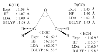
Figure 2: Comparison of HF/6-311G^∗∗(2d,2p), B3LYP/6-311G^∗∗(2d,2p), and LDA/6-311G^∗∗(2d,2p) optimized geometries with the experimental gas phase geometry from Ref. H47 . Note that the structure has $C_{2v}$ symmetry.

The first step towards calculating the electronic absorption spectrum of oxirane is the optimization of the geometry of the gas phase molecule. This was carried out using the HF method and DFT using the LDA and B3LYP functionals. The calculated results are compared in Fig. 2 with the known experimental values. It is seen that electron correlation included in DFT shortens bond lengths, bringing the DFT optimized geometries into considerably better agreement with the experimental geometries than are the HF optimized geometries. This better agreement between DFT and experiment also holds for bond angles. There is not much difference between the LDA and B3LYP geometries with the exception of the COC bond angle which is somewhat better described with the B3LYP than with the LDA functional.

Table 1: Principal oxirane singlet excitation energies (eV) and oscillator strengths (unitless).

TDHF	TDLDA	TDB3LYP	Expt.
9.14 (0.0007)	6.01 (0.0309)	6.69 (0.0266)	7.24(s)
9.26 (0.0050)	6.73 (0.0048)	7.14 (0.0060)	7.45(w)
9.36 (0.0635)	6.78 (0.0252)	7.36 (0.0218)	7.88(s), 7.89(s)
9.56 (0.0635)	7.61 (0.0035)	7.85 (0.0052)
9.90 (0.0478)	7.78 (0.0304)	8.37 (0.0505)
9.93 (0.0935)	8.13 (0.0014)	8.39 (0.0168)
8.15 (0.0405)	8.40 (0.0419)

Several experimental studies of the absorption spectrum of oxirane are available LD49 ; LW58 ; FAHP59 ; BRK+69 ; BBG+92 . The positions of the principal electronic excitations were identified early on but their assignment took a bit longer. The accepted interpretation is based on the study by Basch et al. BRK+69 who combined information from vacuum ultraviolet spectra, photoelectron spectra, and quantum chemical computations, and assigned the observed transitions to O($n$) $\rightarrow$ $3s$ and $3p$ Rydberg transitions. Let us see how this is reflected in our calculations.

While theoretical absorption spectra are often shifted with respect to experimental absorption spectra, we expect to find two strong absorptions in the low energy spectrum, separated from each other by about 0.65 eV. Vertical absorption spectra are calculated using TDHF, TDLDA, and TDB3LYP, all at the B3LYP-optimized geometry. The results are shown in Table 1. TDB3LYP is the method in best agreement with experiments, yielding two strong absorptions red-shifted from experiment by about 0.5 eV and separated by 0.67 eV. The TDLDA method is qualitatively similar, apart from a stronger red shift. In particular, the TDLDA method shows two strong absorptions red-shifted from experiment by about 1.1 eV and separated by 0.78 eV. In contrast, the TDHF spectrum is blue-shifted by about 2 eV and is otherwise of questionable value for interpreting the experimental spectrum. In what follows, we have decided to assign the lowest three absorptions using the results of our TDB3LYP calculations.

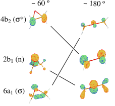
Figure 3: B3LYP MOs. Left: ring structure. Right: open structure.

This first involves an examination of the B3LYP molecular orbitals (MOs). These orbitals are shown in Fig. 3. The electronic configuration of the ring structure is,

$$\cdots[6a_{1}(\sigma)]^{2}[2b_{1}(n)]^{2}[7a_{1}(3s)]^{0}[4b_{2}(\sigma^{*})]^{0}\cdots\,.$$ (10)

The group theoretic MO labels ($a_{1}$, $a_{2}$, $b_{1}$, and $b_{2}$) correspond to representations of the $C_{2v}$ symmetry group. The additional labels, $\sigma$, $n$, and $\sigma^{*}$, show our chemical interpretation of the B3LYP orbitals and their correspondence with the MOs in the WH three-orbital model.

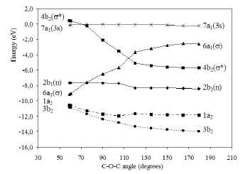
Figure 4: Walsh diagram for $C_{2v}$ ring opening calculated at the B3LYP level. To construct this diagram, the COC bond angle was varied and all other geometric parameters were relaxed within the constraint of $C_{2v}$ symmetry. The HOMO is the $2b_{1}$ orbital on the left hand side and the $4b_{2}$ orbital on the right hand side.

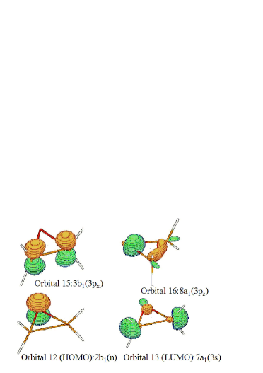
Figure 5: B3LYP MOs implicated in the principal UV absorptions.

Confirmation of the chemical nature of our B3LYP MOs was obtained by constructing a Walsh diagram for $C_{2v}$ ring opening. This graph of MO energies as a function of ring-opening angle ($\alpha$) is shown in Fig. 4. As the ring opens, the C($2p$) $6a_{1}(\sigma)$ bond breaks and so increases in energy. At the same time, the C($2p$) $4b_{2}(\sigma^{*})$ antibond becomes less antibonding and so decreases in energy. The O($2p$) lone pair $2b_{1}(n)$ is not involved in bonding and so maintains a roughly constant energy throughout the ring-opening process. Experimental information about occupied MOs is available from electron momentum spectroscopy (EMS) via the target Kohn-Sham approximation DCCS94 . The ordering of the B3LYP occupied orbitals is consistent with the results of a recent EMS study of oxirane WMWB99 . In particular, the two highest energy occupied orbitals are seen to have a dominant $p$-type character. The interpretation of the unoccupied orbitals is more problematic in that the B3LYP unoccupied orbitals in our calculations are not bound (i.e., have positive orbital energies). We are thus attempting to describe a continuum with a finite basis set. It is thus far from obvious that the unoccupied orbital energies will converge to anything meaningful as the finite basis set becomes increasingly complete. The Walsh diagram shows that the $4b_{2}(\sigma^{*})$ unoccupied orbital becomes bound for ring opening angles beyond about 80^∘. It is also rather localized and hence it makes sense to assign it some physical meaning. This is certainly consistent with previous HF studies using the STO-3G minimal basis set BSD79a and the more extensive 6-31G** basis sets HSS01 . Since our 6-311++G**(2d,2p) basis set is even larger, it is not too surprising that we find an additional unoccupied orbital, namely the $7a_{1}(3s)$ orbital shown in Fig. 5. Although apparently at least partially localized, this orbital remains unbound at all bond angles in the Walsh diagram and care should be taken not to overinterpret its physical nature. Nevertheless this $7a_{1}(3s)$ orbital intervenes in an important way in the interpretation of our calculated electronic absorption spectra and it is upon analysis of the spectra that we will be able to associate this orbital with the $3s$ Rydberg state.

One should also be conscious in using the calculated TDB3LYP absorption spectrum to assign the experimental gas phase UV spectrum that the TDDFT ionization continuum begins at minus the value of the HOMO orbital energy CJCS98 . The value of $-\epsilon_{\text{HOMO}}$ obtained in the different calculations is 6.40 eV with the LDA, 7.68 eV with the B3LYP hybrid functional, and 12.27 eV with HF. As expected from Koopmans’ theorem, the HF value of $-\epsilon_{\text{HOMO}}$ is in reasonable agreement with the experimental ionization potential of 10.57 eV NCK77 . The presence of a fraction of HF exchange in the B3LYP hybrid functional helps to explain why its value of $-\epsilon_{\text{HOMO}}$ lies between that of the pure DFT LDA and that of HF. As far as our TDB3LYP calculations are concerned, the value of $-\epsilon_{\text{HOMO}}$ means that assignment of experimental excitation energies higher than 7.7 eV should be avoided. Fortunately this still allows us to assign the first singlet excitation energies. Examination of the TDB3LYP coefficients yields the following assignments for the three principal UV absorption peaks:

6.69 eV $$: 1^{1}B_{1}[2b_{1}(n)\rightarrow 7a_{1}(3s)]$$ (11)

7.14 eV $$: 2^{1}B_{1}[2b_{1}(n)\rightarrow 8a_{1}(3p_{z})]$$ (12)

7.36 eV $$: 2^{1}A_{1}[2b_{1}(n)\rightarrow 3b_{1}(3p_{x})]\,.$$ (13)

Comparison with the experimental assignment of Basch et al. justifies the identification of these orbitals with the Rydberg orbitals $3s$, $3p_{z}$, and $3p_{x}$.

It is worth pointing out that the expected ${}^{1}[2b_{1}(n),4b_{2}(\sigma^{*})]$ excitation is of ${}^{1}A_{2}$ symmetry and as such corresponds to a spectroscopically forbidden transition. It is in any event fairly high in energy (9.77 eV with TDHF). The ${}^{1}[6a_{1}(\sigma),4b_{2}(\sigma^{*})]$ transition has ${}^{1}B_{2}$ symmetry and so is spectroscopically allowed, but is still found at fairly high energy in our calculations (8.15 eV with TDLDA, 8.37 with TDB3LYP, and 9.93 with TDHF).

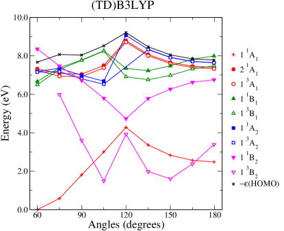
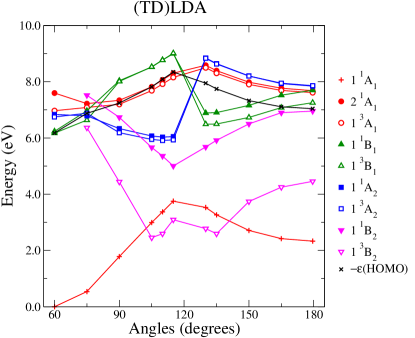
Figure 6: $C_{2v}$ ring opening curves: ground state ($1^{1}A_{1}$) curve calculated using the B3LYP (Gaussian) or the LDA (deMon2k) functional, lowest excited state curve of each symmetry ($2^{1}A_{1}$, $1^{3}A_{1}$, $1^{1}B_{1}$, $1^{3}B_{1}$, $1^{1}A_{2}$, $1^{3}A_{2}$, $1^{1}B_{2}$, and $1^{3}B_{2}$) calculated using the TDB3LYP (Gaussian) and the TDLDA (deMon2k) excitation energies added to the B3LYP and the LDA ground state energy, respectively. The energy zero has been chosen to be the ground state energy for the 60^∘ structure. Note that the “negative excitation energies” for the $1^{3}B_{2}$ state relative to the ground state are really imaginary excitation energies (see text). Also shown is the TDDFT ionization threshold at $-\epsilon_{\text{HOMO}}$.

V.2 $C_{2v}$ Ring-Opening

We now consider how DFT performs for describing the ground state and how well TDDFT performs for describing the lowest excited state of each symmetry for $C_{2v}$ ring-opening of oxirane. Comparisons are made against CASSCF and against high-quality DMC energies calculated at the same geometries. All geometries along the $C_{2v}$ pathway have been fully optimized at each O - C - O ring-opening angle ($\alpha$) using the B3LYP functional. The orbital energies as a function of ring opening angle have already been given in the Walsh diagram (Fig. 4).

Fig. 6 shows the TDB3LYP and TDLDA curves for the ground ($1^{1}A_{1}$) state and the lowest excited-states of each symmetry ($2^{1}A_{1}$, $1^{3}A_{1}$, $1^{1}B_{1}$, $1^{3}B_{1}$, $1^{1}A_{2}$, $1^{3}A_{2}$, $1^{1}B_{2}$, and $1^{3}B_{2}$). Several things are worth noting here. The first point is that, some of the differences between the TDB3LYP and TDLDA curves are apparent, not real, as the points for the two graphs were not calculated at exactly the same angles. In particular, the TDLDA misses the point at 120^∘ where we encountered serious convergence difficulties due to a quasidegeneracy of $\sigma$ and $\sigma^{*}$ orbitals (Fig. 4). Under these circumstances, the HOMO, which suffers from self-interaction errors, can lie higher than the self-interaction-free LUMO. As the program tries to fill the orbitals according to the usual aufbau principle, electron density sloshes on each iteration between the two orbitals making convergence impossible without special algorithms. The TDB3LYP calculations were found to be easier to converge, presumably because they have less self-interaction error.

The second point is that only deMon2k TDLDA calculations are reported here, although we have also calculated TDLDA curves using Gaussian and found similar results when both programs printed out the same information. Unfortunately, Gaussian did not always print out the lowest triplet excitation energy, so we prefer to report our more complete deMon2k results.

The third point is the presence of a triplet instability. This means that, going away from the equilibrium geometry, the square of the first triplet excitation energy decreases, becomes zero, and then negative. The exact meaning of triplet instabilities will be discussed further below. For now, note that we follow the usual practice for response calculations by indicating an imaginary excitation energy as a negative excitation energy. However it is important to keep in mind that a negative excitation energy in this context is only a common convention and not a physical reality. Incidentally, we presume that triplet instability is the source of the difficulty with the Gaussian output mentioned above–the associated coefficients become more complicated and Gaussian may have difficulty analyzing them.

A fourth and final point is that the TDDFT ionization threshold occurs at minus the value of the HOMO energy which is significantly underestimated with ordinary functionals such as the LDA and B3LYP CJCS98 . This artificially low ionization threshold is indicated in the two graphs in Fig. 6. In the TDB3LYP case, the TDDFT ionization threshold is high enough that it is not a particular worry. In the TDLDA case, the TDDFT ionization threshold is lower by about 1 eV. This may explain some of the quantitative differences between the high-lying TDB3LYP and TDLDA curves, although by and large the two calculations give results in reasonable qualitative, and even semi-quantitative, agreement.

We now wish to interpret the TDDFT curves. TDDFT excitations may be characterized in terms of single electron excitations from occupied to unoccupied MOs C95 . Unlike in HF, unoccupied and occupied orbitals in pure DFT (e.g., the LDA) see very similar potentials and hence the same number of electrons. This means that the orbitals are preprepared for describing electron excitations and that simple orbital energy differences are often a good first approximation to describing excitation energies. In the two-orbital model and pure DFT, the singlet, $\omega_{S}$, and triplet, $\omega_{T}$, TDDFT excitation energies for the transition from orbital $i$ to orbital $a$ are,

$$\omega_{S} = \sqrt{\left(\epsilon_{a}-\epsilon_{i}\right)\left[\left(\epsilon_{a}-\epsilon_{i}\right)+2(ia|2f_{H}+f_{xc}^{\uparrow,\uparrow}+f_{xc}^{\uparrow,\downarrow}|ai)\right]}$$

$$\omega_{T} = \sqrt{\left(\epsilon_{a}-\epsilon_{i}\right)\left[\left(\epsilon_{a}-\epsilon_{i}\right)+2(ia|f_{xc}^{\uparrow,\uparrow}-f_{xc}^{\uparrow,\downarrow}|ai)\right]}\,.$$ (14)

In the TDA, this becomes

$$\left(\omega_{S}\right)_{\text{TDA}} = \left(\epsilon_{a}-\epsilon_{i}\right)+(ia|2f_{H}+f_{xc}^{\uparrow,\uparrow}+f_{xc}^{\uparrow,\downarrow}|ai)$$

$$\left(\omega_{T}\right)_{\text{TDA}} = \left(\epsilon_{a}-\epsilon_{i}\right)+(ia|f_{xc}^{\uparrow,\uparrow}-f_{xc}^{\uparrow,\downarrow}|ai)\,,$$ (15)

from which it is clear from the sizes and signs of the integrals that,

$$\left(\omega_{T}\right)_{\text{TDA}}\leq\epsilon_{a}-\epsilon_{i}\leq\left(\omega_{S}\right)_{\text{TDA}}\,.$$ (16)

For Rydberg states the inequalities become near equalities because the overlap of orbitals $i$ and $a$ goes to zero. While no longer strictly valid, these general ideas are still good starting points for understanding results obtained with the hybrid functional B3LYP.

The frontier MOs shown in the Walsh diagram (Fig. 4) supplemented with the addition of the two additional Rydberg orbitals, $3b_{1}(3p_{x})$ and $5b_{2}(3p_{y})$, provides a useful model not only for interpreting the results of our TDDFT calculations, but also for constructing the active space necessary for the CASSCF calculations used to construct the QMC wavefunctions. Fig. 7 shows the results of our best QMC calculation and of the results of the CAS(4,6) calculation on which it is based. For the most part, the CAS and DMC curves differ quantitatively but not qualitatively. The exceptions are the $1^{3}A_{1}$ and $1^{1}B_{2}$ curves where the DMC results, which are significantly lower than the corresponding CAS(4,6) results at some geometries, contain important amounts of dynamic correlation not present at the CAS(4,6) level of calculation. In the remaining graphs (except for Fig. 9) we will suppress CAS(4,6) curves in favor of presenting only the higher quality DMC curves since these offer the better comparison with TDDFT.

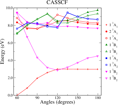
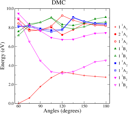
Figure 7: $C_{2v}$ ring opening curves calculated with CASSCF and DMC: curves for the lowest state of each symmetry ($1^{1}A_{1}$, $1^{3}A_{1}$, $1^{1}B_{1}$, $1^{3}B_{1}$, $1^{1}A_{2}$, $1^{3}A_{2}$, $1^{1}B_{2}$, and $1^{3}B_{2}$) are calculated using CAS(4,6) without state averaging, while the $2^{1}A_{1}$ is the result of adding the excitation energy from a state averaged calculation to the ground state $1^{1}A_{1}$ curve calculated without state averaging. The energy zero has been chosen to be the ground state energy for the 60^∘ structure. Note that the negative excitation energies for the $1^{3}B_{2}$ state relative to the ground state are really negative excitation energies. Numerical DMC energies are listed in Appendix B.

We now give a detailed comparison of our TDDFT results with DMC methods, dividing the states into three sets. The first set consists of states where double excitations (lacking in the TDDFT adiabatic approximation) are likely to be important. The second set consists of states which show the effects of triplet instabilities. And the third set consists of Rydberg excitations.

The states of $A_{1}$ symmetry are those most likely to be affected by the absence of double excitations. Although not shown here, we have constructed the two HF curves obtained by enforcing a double occupancy of either the $6a_{1}(\sigma)$ or the $4b_{2}(\sigma^{*})$ orbital. Both single determinants have ${}^{1}A_{1}$ symmetry. The two curves thus generated simply cross at about 120^∘. In the absence of configuration mixing, the ground state curve always follows the lower state and shows an important cusp at 120^∘. Introducing configuration mixing via a CASSCF calculation leads to an avoided crossing.

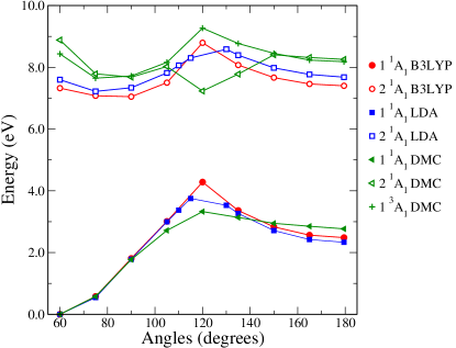
Figure 8: $C_{2v}$ ring opening curves: $1^{1}A_{1}$ and $2^{1}A_{1}$ states. Note that the $1^{3}A_{1}$ state has also been included at the DMC level of calculation.

Now, DFT is different from HF because DFT is exact when the functional $E_{xc}$ is exact while HF always remains an approximation. On the other hand, the Kohn-Sham equations of modern DFT resemble the HF equations and tend to inherit some of their faults when approximate functionals are used. Fig. 8 shows the comparable curves at the TDDFT and DMC levels. As expected, the unphysical cusp is absent in the $1^{1}A_{1}$ ground state curve at the DMC level of calculation. The unphysical cusp is present at both the B3LYP and LDA levels where significant divergences between the DFT and DMC calculations occur between about 100^∘ and 150^∘. However, this region is very much reduced compared to what we have observed to happen for the HF curve where significant divergences beginning at about 75^∘. This is consistent with the idea that even DFT with approximate functionals still includes a large degree of electron correlation.

As to the $2^{1}A_{1}$ excited state curve, only the DMC calculation shows an indication of an avoided crossing. The inclusion of the $1^{3}A_{1}$ excited state curve calculated at the DMC level helps to give a more complete understanding of the curve for this state. Below about 100^∘ and above about 150^∘, the $2^{1}A_{1}$ and $1^{3}A_{1}$ states have nearly the same energy, consistent with the idea that these correspond to the ${}^{1}[a_{1}(\sigma),a_{1}(3s)]$ Rydberg transition below 110^∘ and to the ${}^{1}[b_{2}(\sigma^{*}),b_{2}(3p_{z})]$ Rydberg transition above 150^∘. In between the ${}^{1}[a_{1}(\sigma)^{2},b_{2}(\sigma^{*})^{2}]$ two-electron valence excitation cuts across the ${}^{1}A_{1}$ manifold. The TDDFT calculations are qualitatively capable of describing these one-electron Rydberg excitations but not of describing the two-electron excitation in the bond-breaking region. As expected, the cusp in the DFT $1^{1}A_{1}$ ground state curve is simply reflected as cusps in the TDDFT $2^{1}A_{1}$ excited-state curve.

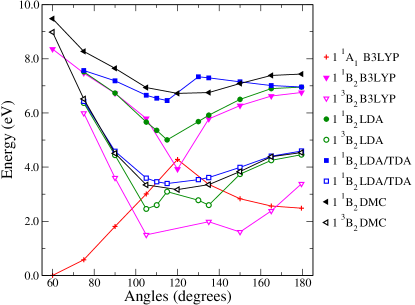
Figure 9: $C_{2v}$ ring opening curves: $1^{3}B_{2}$ and $1^{1}B_{2}$ states. Note that the ground state ($1^{1}A_{1}$) curve has only been shown for the B3LYP calculation since the LDA curve is nearly identical.

The only state which shows triplet instabilities is the $1^{3}B_{2}$ state. The TDLDA $1^{3}B_{2}$ energies are imaginary (even if designated as negative in Figs. 6 and 9) between about about 100^∘ and about 140^∘ while the TDB3LYP $1^{3}B_{2}$ energies are imaginary over a larger range, between about 90^∘ and 160^∘. Certainly, one way to understand how this can happen is through the formulae Eq. (14), but a better way to understand triplet instabilities is in terms of the fact that the quality of response theory energies depends upon having a high-quality ground state. Problems occur in TDDFT excitation energies because the functional $E_{xc}$ is only approximate.

Stability analysis and triplet instabilities have already been discussed in a general way in Sec. II where it was seen that no symmetry breaking is expected for a closed-shell singlet ground state when $E_{xc}$ is exact. However, symmetry breaking can occur when $E_{xc}$ is approximate. To deepen our understanding of triplet instabilities, let us look at a two-orbital model for the dissociation of the $\sigma$ bond in H₂, which is similar to the dissociation of the CC $\sigma$ bond in oxirane. Here we follow the argument in Ref. CGG+00 and consider the wave function,

$$\Psi_{\lambda}=|\sqrt{1-\lambda^{2}}\sigma+\lambda\sigma^{*},\sqrt{1-\lambda^{2}}\bar{\sigma}-\lambda\bar{\sigma}^{*}|\,,$$ (17)

which becomes $|s_{A},\bar{s}_{B}|$ as $\lambda\rightarrow 1/\sqrt{2}$. The corresponding energy expression is,

$$E_{\lambda}=E_{0}+2\lambda^{2}\frac{\omega_{T}^{2}}{\epsilon_{\sigma^{*}}-\epsilon_{\sigma}}+{\cal O}(\lambda^{3})\,.$$ (18)

This result suggests the more general result C01 that symmetry breaking will occur if and only if there is an imaginary triplet excitation energy ($\omega_{T}^{2}<0$). Certainly, one way to overcome the problem of triplet excitation energies is to improve the quality of the exchange-correlation functional. However, another way is to use the TDA. The reason is clear in HF theory where TDHF/TDA is the same as CIS, whose excited states are a rigorous upper bound to the true excitation energies. Therefore, not only will the excitations remain real but variational collapse will not occur. To our knowledge, there is no way to extend these ideas to justify the use of the TDA in the context of TDDFT calculations except by carrying out explicit calculations to show that the TDA yields improved PESs for TDDFT calculations. This was previously shown for H₂ CGG+00 and is evidently also true for oxirane judging from Fig. 9 where the TDLDA/TDA curve is remarkably similar to the DMC curve.

As shown in Fig. 9, triplet instabilities are often also associated with singlet near instabilities. In this case, the TDDFT $1^{1}B_{2}$ singlet excitation energies are much too low. The TDA brings the TDLDA curve into the same energetic region of space as the corresponding DMC curve, but still compared with the DMC curve the TDLDA TDA curve appears to be qualitatively incorrect after 120^∘ where it is seen to be decreasing, rather than increasing, in energy as the angle opens. This, in fact, is the behavior observed in the CAS(4,6) singlet calculation but is opposite to what happens in the more accurate DMC calculation.

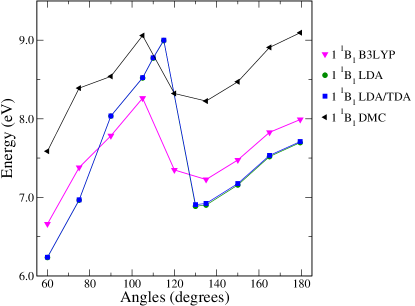
Figure 10: $C_{2v}$ ring opening curves: $1^{1}B_{1}$ state. The TDLDA and TDLDA/TDA curves are practically superimposed.

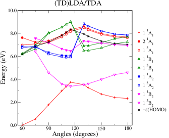
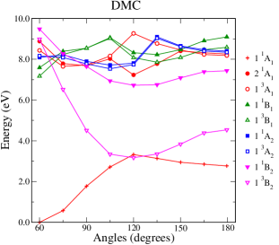
Figure 11: Comparison of TDLDA/TDA and DMC $C_{2v}$ ring opening curves.

The remaining $1^{1,3}B_{1}$ and $1^{1,3}A_{2}$ states are primarily Rydberg in nature with the corresponding singlets and triplets being energetically nearly degenerate. The graph for a single one of these states suffices to illustrate the general trend observed in the case of all four states. Fig. 10 shows what happens for the $1^{1}B_{1}$ states. All the curves have qualitatively the same form. This is particularly true for the TDB3LYP curve which closely resembles the DMC curve but shifted down by a little over one eV in energy. Notice also that the TDLDA and TDLDA/TDA curves are essentially superimposed. This is because,

$$\left(\omega_{S}\right)_{TDA}^{2}-\omega_{S}^{2} = (ia|2f_{H}+f_{xc}^{\uparrow,\uparrow}+f_{xc}^{\uparrow,\downarrow}|ai)^{2}$$

$$\left(\omega_{T}\right)_{TDA}^{2}-\omega_{T}^{2} = (ia|f_{xc}^{\uparrow,\uparrow}-f_{xc}^{\uparrow,\downarrow}|ai)^{2}\,.$$ (19)

For Rydberg states the overlap between orbitals $i$ and $a$ is very small and so the difference between full and TDA TDLDA calculations can be neglected. From Eq. (13) this also means that the Rydberg excitation energies also reduce to simple orbital energy differences.

Fig. 11 shows that the TDLDA/TDA yields, at least in this case, a mostly qualitatively reasonable description of photochemically important PESs as compared with high-quality QMC PESs. By this we only mean that corresponding TDLDA/TDA and QMC potential energy curves have typically the same overall form and are found at roughly similar energies. As discussed above, significant differences do remain in the shapes of some potential energy curves ($2^{1}A_{1}$ and $1^{1}B_{2}$) and the detailed energy ordering of the curves differs between the TDLDA/TDA and QMC results.

V.3 Con- and Disrotatory Ring Opening

Conrotatory and disrotatory potential energy surfaces were calculated using the simplifying assumption that each set of 4 atoms OCH₂ is constrained to lie in a plane. Our coordinate system is defined in Fig. 12. All other geometrical parameters were relaxed for the thermal reaction preserving $C_{s}$ and $C_{2}$ symmetry for the con and the dis path, respectively.

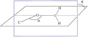
Figure 12: $(\alpha,\theta)$ coordinate system used in this paper.

V.3.1 Thermal Reaction

Fig. 13 shows the ground state ($S_{0}$) PES. In accordance with the WH model there appears to be a much lower energy barrier for con ring opening than for dis ring opening. Also shown is the lowest triplet state ($T_{1}$). It is clear that triplet instabilities occur along the disrotatory pathway as the CC $\sigma$ bond breaks. Remarkably, they do not occur along the conrotatory pathway in the LDA. (They should, of course, be absent when the exchange-correlation functional is exact.) Although triplet instabilities account for about 50% of the LDA surface, this fraction actually increases to 93% for the B3LYP functional where triplet instabilities occur along both the conrotatory and disrotatory reaction pathways. Finally, when the HF method is used triplet instabilities account for 100% of the PES. Perhaps because we forced the OCH₂ to lie in a single plane, triplet instabilities appear to be nearly everywhere in these last methods, potentially spelling trouble for mixed TDDFT/classical photodynamics calculations. We would thus like to caution against the use of hybrid functionals for this type of application. At the same time, we reiterate our recommendation to use the TDA because, of course, the TDLDA/TDA excited state PESs (Fig. 14) show no triplet instabilities.

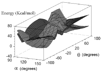
Figure 13: TDLDA $S_{0}$ (light grey) and $T_{1}$ (dark grey) PESs. Note that a “negative excitation energy” is just a convenient graphical trick for representing an imaginary excitation energy. Negative excitation energies correspond to triplet instabilities.

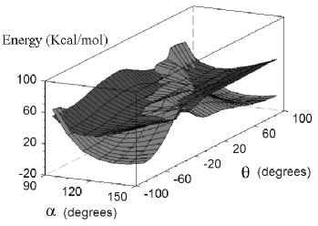
Figure 14: TDLDA/TDA $S_{0}$ (light grey) and $T_{1}$ (dark grey) PESs. In this case negative excitation energies are real, not imaginary, quantities.

V.3.2 Photochemical Reaction

In considering whether the WH model has any validity for describing con- versus disrotatory rotation for photochemical ring opening in oxirane, we are immediately faced with the problem that there are a large number of excited states with similar energies which cross each other (Fig. 7). Provisionally, we have decided to assume that state symmetry is conserved and so to look only at one PES, namely the $1^{1}B_{1}S_{1}$ surface (which we shall simply refer to as $S_{1}$) which begins as the ${}^{1}[2b_{1}(n)\rightarrow 7a_{1}(3s)]$ excitation for the closed cycle and then evolves as the molecular geometry changes. In so doing, we are following the spirit of simple WH theory which makes maximum use of symmetry. Turning back to this theory (Fig. 1) and thinking of excitation to a Rydberg state as analogous to electron removal, it suffices to remove an electron from the $n$ orbital of the thermal WH diagram, thereby giving the $\sigma^{2}n^{1}$ configuration, to have an idea of what might be the relative importance of the con and dis mechanisms for the $S_{1}$ surface. In this case the con mechanism leads to the energetically nearest-neighbor single excitation, $\sigma\rightarrow n$, and the dis mechanism leads to the nearest-neighbor single excitation, $\sigma\rightarrow\sigma^{*}$. Since both mechanisms correspond to nearest-neighbor excitation, no particular preference is a priori expected for one mechanism over the other. The ground ($S_{0}$) and excited state singlet ($S_{1}$) surfaces calculated with the TDLDA/TDA are shown in Fig. 15. Indeed the simple WH theory appears to be confirmed in that the $S_{1}$ surface is remarkably flat.

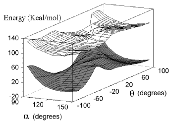
Figure 15: TDLDA/TDA $S_{0}$ (light grey) and $S_{1}$ (white) potential energy surfaces.

Unfortunately this analysis is far too simplistic. In particular, Kasha’s rule K50 tells us that the first excited triplet ($T_{1}$) or singlet ($S_{1}$) states are the most likely candidates for the initiation of a photochemical reaction, where now $T_{1}$ and $S_{1}$ are the globally lowest states and not necessarily the lowest state of a given symmetry. This is based upon the idea that relaxation of higher excited states is rapid. Such relaxation is due to environmental effects or vibronic coupling which need not preserve the symmetry of the electronic state. Hence $S_{1}$ at one geometry is not necessarily $S_{1}$ at another geometry. Indeed looking again at the DMC curves in Fig. 7, it is easy to believe that the molecule will eventually arrive in the $1^{1}B_{2}(\sigma,\sigma^{*})$ state during ring opening and that, because the $\sigma$ orbital is higher in energy than the $\sigma^{*}$ orbital at this geometry (Fig. 4), that the usual WH argument will still predict a preference for the dis mechanism.

Again we are falling into a trap imposed by the use of symmetry. Excitation, for example, from the $2b_{1}(n)$ orbital (Fig. 3) into the $8a_{1}(3p_{z})$ Rydberg orbital (Fig. 5) might lead to preferential CO, rather than CC, bond breaking to the extent that ring opening augments the valence CO($\sigma*$) character of the target orbital T07 . The difficulty of predicting a priori such behavior is part of what motivates us to move towards dynamics as a better tool for photochemical modeling.

VI Conclusion

In this paper, we have examined the potential energy curves and surfaces for the symmetric ring opening of oxirane to assess possible difficulties which might be encountered when using TDDFT in photodynamics simulations of its photochemistry. Our TDDFT calculations provided useful insight helpful in constructing the active space needed for more accurate CASSCF and still more accurate DMC calculations. It is indeed worth noting that identifying active spaces is probably one of the more common uses of TDDFT in photochemical studies. Here, we summarize our main conclusions obtained by comparing our TDDFT and DMC results.

Oxirane does not seem to be a molecule where charge transfer excitations are important. The artificially low ionization threshold typical in TDDFT for most functionals is still high enough for the B3LYP functional so as not to pose a serious problem. Even for the LDA functional, where the TDDFT ionization threshold is lower, the shapes of the excited-state Rydberg curves seem to be qualitatively correct even if they should not be considered quantitative.

Problems do show up as the CC $\sigma$ bond breaks. By far, the most severe problem encountered is the presence of triplet instabilities and singlet near instabilities, where the excited-state PES takes an unphysical dive in energy towards the ground state. In the case of the triplet, the excitation energy may even become imaginary, indicating that the ground state energy could be further lowered by allowing the Kohn-Sham orbitals to break symmetry. Although this problem is very much diminished compared to that seen in the HF ground state, it is still very much a problem as seen for example in the 2D surfaces of the con and disrotatory ring opening of oxirane.

It is difficult to overstate the gravity of the triplet instability problem for the use of TDDFT in photodynamics simulations. One should not allow symmetry breaking as it is an artifact which should not occur when the exchange-correlation functional is exact. Moreover, there may be more than one way to lower the molecular energy by breaking symmetry, and searching for the lowest energy symmetry broken solution can be time consuming. Finally, the assignment of excited states using broken symmetry orbitals is far from evident. On the whole, it thus seems better to avoid the problem by using the TDA to decouple (at least partially) the quality of the excited-state PES from that of the ground state PES. Our calculations show that this works remarkably well for the $1^{3}B_{2}$ curve along the $C_{2v}$ pathway, in comparison with good DMC results. The $1^{1}B_{2}$ state, which appeared to collapse in energy without the TDA in the region of bond breaking, is also restored to a more reasonable range of energies. For this reason, we cannot even imagine carrying out photochemical simulations with TDDFT without the use of the TDA. Or, to put it more bluntly, the TDA, which is often regarded as an approximation on conventional TDDFT calculations, gives better results than does conventional TDDFT when it comes to excited-states PESs in situations where bond breaking occurs.

The TDA is unable to solve another problem which occurs as the CC $\sigma$ bond breaks, namely the presence of an unphysical cusp on the ground state curve (or surface). This cusp is there because of the difficulty of approximate density functionals to describe a biradical structure with a single determinantal wave function. The cusp is also translated up onto the excited-state curves because of the way that PESs are constructed in TDDFT. However the problem is very much diminished compared to that seen in HF because of the presence of some correlation in DFT even when the exchange-correlation functional is approximate. The ultimate solution to the cusp problem is most likely some sort of explicit incorporation into TDDFT of two- and higher-electron excitations. Among the methods proposed for doing just this are dressed TDDFT or polarization propagator corrections CZMB04 ; MZCB04 ; C05 and spin-flip TDDFT SHK03 ; SK03 ; WZ04 .

Our examination of the con- and disrotatory ring-opening pathways revealed another important point which has nothing to do with TDDFT. This is that the manifold of excited state PESs is too complicated to interpret easily. The best way around this is to move from a PES interpretation to a pathway interpretation of photochemistry, and the best way to find the pathways moving along and between adiabatic PESs seems to be to carry out dynamics. For now, it looks as though the use of TDDFT/TDA in photodynamics simulations may suffice to describe the principal photochemical processes in oxirane. On-going calculations T07 do indeed seem to confirm this assertion in so far as trajectories have been found in good agreement with the accepted Gomer-Noyes mechanism GN50 ; IIT73 .

Appendix A Photochemistry of Oxiranes

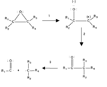
Figure 16: Typical reactions of alkyl oxiranes.

The generic structure of oxiranes is shown as the starting point in the chemical reactions in Figs. 16 and 17. When R₁, R₂, R₃, and R₄ are hydrogens or alkyl groups, then the prefered reaction is CO cleavage both photochemically and thermally (Step 1, Fig. 16). In particular it is estimated that the CO rupture energy is about 52 kcal/mol while the CC rupture energy is 5-7 kcal/mol higher BSD79a . Since the molecule is not symmetric along the CO ring-opening pathway, the WH model does not apply. Photochemical CO ring opening may be followed by alkyl migration AWR+04 (Step 2, Fig. 16). In the particular case of oxirane itself (R₁=R₂=R₃=R₄=H), hydrogen migration is followed by breaking of the CC single bond (Step 3, Fig. 16). This is the Gomer-Noyes mechanism GN50 which was confirmed experimentally by Ibuki, Inasaki, and Takesaki IIT73 .

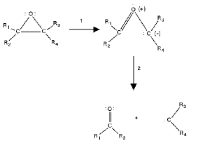
Figure 17: Typical reactions of aryl oxiranes.

In contrast, cyano and aryl substitutions favor CC bond breaking (Step 1, Fig. 17) to form what is often refered to as a 1,3-dipolar species or a carbonyl ylide. This is the case where there may be sufficient symmetry that the WH model applies. The photochemistry of phenyl and phenyl substituted oxiranes has been reviewed in Refs. H77 ; HRS+80 ; P87 and on pages 565-566 of Ref. T91 . Evidence for carbonyl ylides goes back to at least the 1960s when Ullman and Milks investigated the tautomerization of 2,3-diphenylindenone oxide UM62 ; UM64 and Linn and Benson investigated the ring-opening reaction of tetracyanoethylene oxide LB65 ; L65 . Finding cases where the WH model applies and where its predictions can be verified turns out to be not straightforward, particularly in the photochemical case. There are several reasons for this. First of all, too much asymmetry should be avoided in order to assure the applicability of the WH orbital symmetry conservation rule and so avoid passing directly onto carbene formation (Step 2, Fig. 17). Secondly, the substituted oxirane should include groups which are bulky enough to confer the structural rigidity needed to avoid premature radiationless relaxation, but not bulky enough to favor carbene formation. The predictions of the WH model have been found to hold for cis- and trans-1,2-diphenyloxirane MP84 while carbene formation dominates for tetraphenyl oxirane TABG80 .

Appendix B Supplementary Material

Benchmark quality diffusion Monte Carlo (DMC) energies calculated at the geometries given in Table 7 are reported here for the ground state ($1^{1}A_{1}$, Tables 2 and 3) and the lowest excited state of each symmetry ($2^{1}A_{1}$, Table 3; $1^{3}A_{1}$, Table 2; $1^{1}B_{1}$, $1^{3}B_{1}$, Table 4; $1^{1}A_{2}$, $2^{3}A_{2}$, Table 5; and $1^{1}B_{2}$, $1^{3}B_{2}$, Table 6). We set the zero of the energy to coincide with the DMC $1^{1}A_{1}$ energy at 60^∘ and report the statistical error on the energy in parenthesis. Note that the negative value of the $1^{1}A_{1}$ SA-DMC energy at 60^∘ is statistically compatible with zero. We hope that these DMC data will encourage further developing and testing of improved TDDFT algorithms suitable for addressing the problems mentioned in this article.

Table 2: $A_{1}$ DMC energies as a function of COC ring-opening angle along the $C_{2v}$ ring-opening pathway.

$A_{1}$ DMC Energies and statistical error in Hartree
$\angle$ COC (∘)	$1^{1}A_{1}$	$1^{3}A_{1}$
60.	0.0000 (0.0009)	0.3099 (0.0010)
75.	0.0212 (0.0009)	0.2811 (0.0010)
90.	0.0651 (0.0010)	0.2836 (0.0009)
105.	0.0998 (0.0010)	0.2998 (0.0010)
120.	0.1222 (0.0009)	0.3406 (0.0011)
135.	0.1153 (0.0009)	0.3223 (0.0009)
150.	0.1083 (0.0009)	0.3106 (0.0010)
165.	0.1048 (0.0010)	0.3025 (0.0010)
179.5	0.1017 (0.0010)	0.3007 (0.0010)

Table 3: ${}^{1}A_{1}$ SA-DMC energies as a function of COC ring-opening angle along the $C_{2v}$ ring-opening pathway.

${}^{1}A_{1}$ SA-DMC Energies and statistical error in Hartree
$\angle$ COC (∘)	$1^{1}A_{1}$	$2^{1}A_{1}$
60.	-0.0018 (0.0009)	0.3246 (0.0009)
75.	0.0254 (0.0010)	0.2904 (0.0009)
90.	0.0694 (0.0010)	0.2865 (0.0010)
105.	0.1011 (0.0010)	0.2962 (0.0009)
120.	0.1263 (0.0009)	0.2699 (0.0010)
135.	0.1196 (0.0010)	0.2902 (0.0010)
150.	0.1103 (0.0010)	0.3109 (0.0011)
165.	0.1054 (0.0010)	0.3063 (0.0010)
179.5	0.1037 (0.0010)	0.3054 (0.0010)

Table 4: $B_{1}$ DMC energies as a function of COC ring-opening angle along the $C_{2v}$ ring-opening pathway.

$B_{1}$ DMC Energies and statistical error in Hartree
$\angle$ COC (∘)	$1^{1}B_{1}$	$1^{3}B_{1}$
60.	0.2788 (0.0010)	0.2636 (0.0010)
75.	0.3083 (0.0009)	0.3026 (0.0010)
90.	0.3138 (0.0010)	0.3140 (0.0009)
105.	0.3329 (0.0010)	0.3316 (0.0010)
120.	0.3058 (0.0010)	0.2970 (0.0010)
135.	0.3023 (0.0010)	0.2887 (0.0010)
150.	0.3113 (0.0010)	0.2972 (0.0010)
165.	0.3274 (0.0010)	0.3111 (0.0011)
179.5	0.3343 (0.0010)	0.3155 (0.0010)

Table 5: $A_{2}$ DMC energies as a function of COC ring-opening angle along the $C_{2v}$ ring-opening pathway.

$A_{2}$ DMC Energies and statistical error in Hartree
$\angle$ COC (∘)	$1^{1}A_{2}$	$1^{3}A_{2}$
60.	0.2972 (0.0010)	0.3001 (0.0009)
75.	0.3021 (0.0010)	0.2971 (0.0009)
90.	0.2901 (0.0010)	0.2857 (0.0010)
105.	0.2835 (0.0010)	0.2769 (0.0010)
120.	0.2870 (0.0010)	0.2843 (0.0010)
135.	0.3344 (0.0010)	0.3319 (0.0011)
150.	0.3179 (0.0010)	0.3165 (0.0010)
165.	0.3111 (0.0010)	0.3088 (0.0010)
179.5	0.3086 (0.0010)	0.3066 (0.0010)

Table 6: $B_{2}$ DMC energies as a function of COC ring-opening angle along the $C_{2v}$ ring-opening pathway.

$B_{2}$ DMC Energies and statistical error in Hartree
$\angle$ COC (∘)	$1^{1}B_{2}$	$1^{3}B_{2}$
60.	0.3484 (0.0009)	0.3301 (0.0010)
75.	0.3040 (0.0010)	0.2395 (0.0010)
90.	0.2810 (0.0010)	0.1657 (0.0010)
105.	0.2549 (0.0011)	0.1229 (0.0009)
120.	0.2470 (0.0011)	0.1165 (0.0010)
135.	0.2481 (0.0010)	0.1232 (0.0009)
150.	0.2604 (0.0010)	0.1410 (0.0010)
165.	0.2718 (0.0010)	0.1611 (0.0009)
179.5	0.2733 (0.0010)	0.1667 (0.0010)

Table 7: Oxirane $C_{2v}$ geometries obtained at different COC ring opening angles with all other parameters optimized at the B3LYP level.

$C_{2v}$ geometries
$\angle$ COC (∘)	$\angle$ HCH (∘)	$\angle$ HCOC (∘)	$R(\mbox{CH})$ (Å)	$R(\mbox{CO})$ (Å)
60.	115.52	111.317	1.08375	1.44558
75.	118.69	105.214	1.08311	1.36333
90.	122.04	97.339	1.08131	1.34639
105.	122.28	84.096	1.08311	1.35811
120.	118.06	109.402	1.08576	1.38032
135.	119.88	105.829	1.08353	1.33439
150.	121.78	101.409	1.08154	1.30455
165.	123.27	96.054	1.08009	1.28694
179.5	123.86	90.207	1.07954	1.28114