Microscopic origin of granular ratcheting

Abstract

Numerical simulations of assemblies of grains under cyclic loading exhibit “granular ratcheting”: a small net deformation occurs with each cycle, leading to a linear accumulation of deformation with cycle number. We show that this is due to a curious property of the most frequently used models of the particle-particle interaction: namely, that the potential energy stored in contacts is path-dependent. There exist closed paths that change the stored energy, even if the particles remain in contact and do not slide. An alternative method for calculating the tangential force removes granular ratcheting.

I Introduction

Granular ratcheting refers to the slow, linear accumulation of strain in a granular sample under cyclic loading. Several versions of this phenomena have been identified. The first variant to be found occurs when the loaded sample reaches the critical state once per cycle. The mechanism is easily understood: the material flows while it is in the critical state, giving rise to a deformation that accumulates with cycle number. However, ratcheting can also appear even when the sample never reaches the critical state Festag . In the following, we discuss exclusively this second type of ratcheting.

Ratcheting in the absence of a critical state has also been observed in numerical simulations Fernando ; Ramon ; Ramon2 ; RamonItaly . This is a very promising development, for one has access to all the quantities in numerical simulations, and it is usually possible to identify the origin of the phenomena. Once this has been done, one can then ask if the cause of the phenomena in the simulations is related to the cause in the experiments.

Numerical studies have already provided many clues to granular ratcheting. The important role of sliding contacts has been pointed out Fernando , granular ratcheting has been delimited from other possible behaviors Ramon , and the influence of various parameters has been studied Ramon2 ; RamonItaly . One finding of these studies is that granular ratcheting is a quasi-static phenomena. Specifically, if one lets the frequency of the oscillating force tend to zero while keeping all other parameters the same, the deformation per cycle approaches a constant.

What is still missing is an understanding of granular ratcheting on the micro-mechanical level: How exactly does the phenomenon arise from interaction of individual particles? Is it possible to modify the particle interaction law to eliminate ratcheting? What is the simplest system needed to produce ratcheting? We answer these questions in this paper.

In Sec. II we show that ratcheting can be obtained with only 16 particles. Ratcheting occurs if a single contact becomes sliding. Previously, ratcheting was linked to the presence of sliding contacts, but this is the first time that it is shown that only a single contact is necessary. We also show that the application of unconventional boundary conditions can lead to ratcheting even when there are no sliding contacts. In Sec. III, we show how granular ratcheting arises from the way tangential forces are calculated. In Sec. IV.1 we present an alternative method that does not exhibit ratcheting. Finally, in the appendix, we show how stiffness matrix theory can illuminate some aspects of the problem.

II Description of granular ratcheting

II.1 Model definition

In this section, we present a very brief description of granular ratcheting, since more complete discussions already exist Ramon2 . Granular ratcheting is observed in biaxial or triaxial tests, where a granular sample is enclosed in a test chamber, and subjected to a uniform pressure and a cyclic load. We consider here exclusively the two dimensional version of these experiments, often called the “biaxial box”, where a granular sample composed of disks is enclosed in a rectangular box of dimensions $L_{x}\times L_{y}$, with forces $F_{x}$ and $F_{y}$ exerted on the walls. The forces are

$$F_{x}=P_{0}L_{y},\quad F_{y}=L_{x}\left[P_{0}+q(t)\right],$$ (1)

where $P_{0}$ is the pressure exerted on the sample, and $q(t)$ is a periodic function, usually sinusoidal. In the simulations presented here, $q(t)=\Delta\sigma(1-\cos\omega t)$. One usually uses deviatoric strain

$$\gamma=\frac{L_{y}}{L_{y0}}-\frac{L_{x}}{L_{x0}},$$ (2)

to characterize the deformation. (Here $L_{x0}$ and $L_{y0}$ are the lengths of the system at the beginning of the simulation.)

We use a common numerical model of granular materials: grains are represented by disks who repel each other when they overlap. Thus whenever two disks touch each other, they exert a repulsive force $F_{n}$ at the point of contact, directed normal to the particle surfaces. $F_{n}$ is an increasing function of the overlap $D_{n}$. If the surfaces of two touching disks move relative to each other in the tangential direction, a second force $F_{t}$ arises, directed tangent to the particle surfaces. $F_{n}$ and $F_{t}$ are called the normal and tangential components of the contact force. In addition to these forces, some damping forces are included to remove energy injected by the loading.

The contact force is subjected to two constraints, namely

$$F_{n}\geq 0,\quad\mu F_{n}\geq|F_{t}|.$$ (3)

The first condition excludes cohesion, and the second is the Coulomb friction law. The constant $\mu$ is the Coulomb friction coefficient. Contacts where $|F_{t}|=\mu F_{n}$ are called sliding contacts, and those where $|F_{t}|<\mu F_{n}$ are called non-sliding.

All studies of granular ratcheting use this model, except sometimes polygons are used instead of disks Fernando .

II.2 Ratcheting with sixteen particles

If one wishes to approximate the continuum-like behavior of soils, simulations with large numbers of particles are necessary. Therefore, granular ratcheting has been studied in assemblies of hundreds or thousands of particles. In this paper, however, we wish simply to discover the origin of the phenomena, so it is useful to consider small numbers of particles. In this section, we study an assembly of sixteen particles that exhibits granular ratcheting. The normal force is taken to be proportional to the overlap area, as in Ref. Ramon2 .

Figure 1: Stress-strain curve of the system with $16$ particles discussed in Sec. II.2.

Figure 2: Accumulated strain for the system shown in Fig. 1.

In Fig. 1 we show a plot of $\gamma$ vs $q$ for a biaxial test performed on sixteen circular particles. In the first cycle, $\gamma$ increases to about $0.008$. During subsequent cycles, the system appears to trace out a four-sided polygon in the $q$-$\gamma$ plane. However, the path is not quite a polygon, because the system does not quite return to its starting point after one cycle, but to one where $\gamma$ is slightly larger. This is made obvious in Fig. 2, where $\gamma$ is plotted at $t=nT$, were $T$ is the period of the cyclic loading, and $n=0,1,2\ldots$. A small, linear increase of $\gamma$ with cycle number is visible. This is granular ratcheting.

During one cycle, all the contacts remain non-sliding, except for one, which becomes sliding twice per cycle. This single contact is responsible for granular ratcheting, for if we inhibit sliding at this contact by increasing $\mu$, granular ratcheting stops. However, we show below that ratcheting can also occur without sliding contacts with slightly different boundary conditions.

Figure 3: A sketch of the sliding contact’s trajectory in its $(F_{n},F_{t})$ plane. The diagonal dotted lines show the Coulomb condition given in Eq. (3).

In Fig. 3, we show the trajectory of the sliding contact in its $(F_{n},F_{t})$ plane. The equalities $|F_{t}|=\mu F_{n}$ are also shown on the graph, and form a cone, with the vertex at the origin. The conditions in Eq. (3) mean that $(F_{n},F_{t})$ must always lie within this cone. As one can see, the ratcheting contact’s trajectory is a trapezoid, with the four corners labeled $A$, $B$, $C$, and $D$. The two parallel line segments correspond to the change in force when all contacts are non-sliding. Line segments $BC$ and $DA$ lie on the sides of the cone $|F_{t}|=\mu F_{n}$, and correspond to times when the contact is sliding with $F_{t}=\mu F_{n}$ or $F_{t}=-\mu F_{n}$ respectively. The trajectory is not quite a trapezoid, because after one cycle, the point does not return to $A$, but arrives at $A^{\prime}$, a bit closer to the origin than, but very close to, $A$. After the following cycle, the system has again shifted towards the origin by the same amount. This shift has its origin in the tiny displacement that occurs with each cycle - the sliding contact is gradually opening.

Figure 4: Trajectories of selected non-sliding contacts in the system shown in Fig. 1.

The non-sliding contacts in the packing also trace out trapezoids, but their edges do not intersect the cone $|F_{t}|=\mu F_{n}$. Some examples are shown in Fig. 4. The corners of these trapezoids correspond to the times when the sliding contact begins or stops sliding. When all contacts remain non-sliding, the trajectories are no longer trapezoids, but straight lines: under loading, each contact force moves on a straight line, and under unloading, it simply retraces its path. The reason for this is given in the appendix.

II.3 Ratcheting without sliding contacts

Figure 5: Strain per cycle under elliptic cyclic loading [see Eqs. (4) and (5)]. The circles are the observed points, and the line is a fit of the form $\Delta\gamma=A\sin\phi$. The simulations were done with 16 particles. Sliding contacts were surpressed by setting $\mu=\infty$.

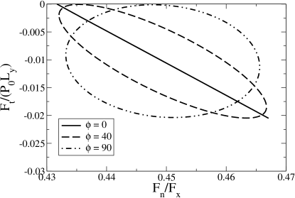
Figure 6: Trajectory of a contact in the $(F_{n},F_{t})$ plane under elliptic cyclic loading, for different values of the phase shift $\phi$ (given in degrees).

When the force on both walls is varied cyclically:

$$F_{x}=L_{y}\left[P_{0}+q_{x}(t)\right],\quad F_{y}=L_{x}\left[P_{0}+q_{y}(t)\right],$$ (4)

ratcheting can occur without sliding contacts. We carried out simulations of a small ($16$ particles) system with Eq. (4), with

$$q_{x}(t)=\Delta\sigma(1-\cos\omega t+\phi),\quad q_{y}(t)=\Delta\sigma(1-\cos\omega t).$$ (5)

Note the presence of a phase shift $\phi$ between $F_{x}$ and $F_{y}$. We call this form of loading elliptic cyclic loading, because ellipses are traced out in the $(F_{x},F_{y})$ plane. During these simulations, sliding was suppressed by setting $\mu=\infty$. The results are shown in Fig. 5. The strain $\Delta\gamma$ per cycle is proportional to $\sin\phi$. If one traces out the path of $q_{x}(t),q_{y}(t)$ in the $q_{x},q_{y}$ plane, then one obtains an ellipse whose area is proportional to $\sin\phi$. Tracing out any contact in the $F_{n},F_{t}$ plane also yields an ellipse proportional to $\sin\phi$. Some examples are shown in Fig. 6. This suggests that ratcheting is related to the area enclosed by trajectories in the $(F_{n},F_{t})$ plane.

II.4 Sign of the strain

Ratcheting with small numbers of particles has another distinguishing property: the strain accumulation can be either positive or negative. Note that in Eq. (1), the average imposed force does not correspond to an isotropic pressure, because $q(t)\geq 0$. The pressure exerted by the walls on the top and bottom of the sample are larger than at the side walls. Thus one expects the sample to be gradually flattened, with the top and bottom walls moving toward each other, while the side walls are pushed apart. This corresponds to $\gamma<0$ in Eq. (2). A series of $100$ different ratcheting simulations with $16$ particles were performed, differing from each other only in the initial condition. Of these $100$ simulations, $71$ exhibited unambiguously ratcheting. Of these $71$ cases ratcheting, $51$ had $\gamma<0$ as expected, but the remaining $20$ had $\gamma>0$.

On the other hand, when the sample size is larger, one has $\gamma<0$ whenever there is ratcheting. A second series of $25$ simulations, this time with $400$ particles, yields $18$ unambiguously ratcheting simulations, all with $\gamma<0$. The range of $\gamma$ observed is also much smaller than for $16$ particles. These results suggest that the strain accumulated by a large sample is some kind of average over strain accumulated by the small regions composing it. In these small regions, there can be either negative or positive strain, but after averaging, these fluctuations are smoothed out, so a large sample has a quite predictable behavior.

Previous studies of granular ratcheting always considered large numbers of particles, so this was never noticed.

III Origin of Ratcheting

III.1 Particle interaction model

We now turn our attention from the description of granular ratcheting to its cause. We will consider a non-sliding contact between two particles subjected to cyclic external forces. To facilitate the analysis, we assume that $F_{n}$ is linear in the overlap distance. One imagines that when two grains first touch, two springs are created, one in the tangential and the other in the normal direction. Both springs obey Hooke’s law so that the normal and tangential contact forces are proportional to the spring elongations $D_{n}$, $D_{t}$:

$$F_{n}=-K_{n}D_{n},\quad F_{t}=-K_{t}D_{t},$$ (6)

where $K_{n}$ and $K_{t}$ are the spring constants. Here, $F_{n}>0$ is interpreted as pushing the particles apart, and $D_{n}<0$ occurs when the particles overlap. Eq. (6) holds only for touching $D_{n}<0$ particles, so $F_{n}>0$ in accord with Eq. (3). On the other hand, $D_{t}$ can have either sign, corresponding to the two opposite tangential directions (up and down in Fig. 7).

The springs are stretched by the relative motion of the particles, as long this does not violate any of the conditions in Eq. (3). When the contact is non-sliding, one has

$$\frac{dD_{n}}{dt}=V_{n},\quad\frac{dD_{t}}{dt}=V_{t},$$ (7)

where $V_{n}$ and $V_{t}$ are just the relative velocities at the point of contact:

$$V_{n} = (\mathbf{v}_{i}-\mathbf{v}_{j})\cdot\mathbf{n},$$ (8)

$$V_{t} = (\mathbf{v}_{i}-\mathbf{v}_{j})\cdot\mathbf{t}-r_{i}\omega_{i}-r_{j}\omega_{j},$$ (9)

where $\mathbf{v}_{i}$, $\omega_{i}$, and $r_{i}$ are the velocity, angular velocity and radius of particle $i$, and $i$ and $j$ label the touching particles. The unit vector $\mathbf{n}$

$$\mathbf{n}=\frac{\mathbf{x}_{i}-\mathbf{x}_{j}}{|\mathbf{x}_{i}-\mathbf{x}_{j}|}$$ (10)

points from particle $j$ toward particle $i$, and $\mathbf{t}$ is a tangent vector. If the two-dimensional space is assumed to be embedded in a three dimensional one, $\mathbf{t}$ can be defined as $\mathbf{t}=\mathbf{z}\times\mathbf{n}$, as shown in Fig. 7. The forces $F_{n}$ and $F_{t}$ are then directed along $\mathbf{n}$ and $\mathbf{t}$ respectively. Note that the signs in Eq. (9) depend on the choice of $\mathbf{n}$, $\mathbf{t}$, and the meaning of positive and negative $D_{t}$. In Fig. 7, $D_{t}>0$ means points attached to particle $i$ move upward relative to points attached to particle $j$.

Figure 7: Definitions for particle interaction laws. The unit vector $\mathbf{n}$ defined in Eq. (10) points from particle $j$ toward particle $i$, and $\mathbf{t}=\mathbf{z}\times\mathbf{n}$, where the $z$ axis points out of the page.

If a contact opens, then $F_{n}=F_{t}=0$ in accord with the first condition of Eq. (3). If two separated particles come together again, there is no memory of the previous contact.

The second condition in Eq. (3) is enforced by setting

$$D_{t}=\pm\mu\frac{K_{n}}{K_{t}}D_{n}$$ (11)

whenever using Eq. (7) would lead to a violation of Eq. (3).

Sliding contacts are accounted for by modifying Eq. (7), but we do not need to consider this in detail, since sliding is not needed for ratcheting to occur, as shown in Sec. II.3.

Note that no damping has been included in Eq. (6). This is because ratcheting is a quasi-static phenomenon. As the frequency of the cyclic loading becomes very long, the deformation per cycle approaches a constant. In the limit of an infinitely long cycle, the particle velocities vanish. Any damping will also vanish, since it is proportional to the velocities. Since ratcheting exists in the limit of infinitely long cycles, one does not need to consider damping in order to understand granular ratcheting. Damping is always included in simulations to model the loss of energy when grains collide or slide against one another.

The model that has been described above has been in use for almost thirty years Cundall79 . It has been used in many different studies, and considered to be well understood. Nevertheless, we show that this model contains an approximation that generates granular ratcheting.

III.2 Path dependent potential energy

Granular ratcheting occurs because the model described in Sec. (III.1) yields a path-dependent potential energy. Here, we are referring to the potential energy stored in a contact when two particles overlap. It models the elastic energy stored when two grains are pushed together. If the force pushing two particles together is suddenly released, this potential energy is converted into kinetic energy, and the particles will separate. When they separate, the highest possible kinetic energy they can attain is

$$E=\frac{1}{2}(K_{n}D_{n}^{2}+K_{t}D_{t}^{2}).$$ (12)

Thus Eq. (12) gives the potential energy stored in the contact.

Figure 8: The origin of granular ratcheting. This figure shows two touching disks. The lower disk is fixed, and the upper disk moves without rotating, its center tracing out the closed path $A\to B\to C\to D\to A$. The contact forces return to their initial state only if the upper particle stops at $A^{\prime}$ instead of proceeding to $A$.

We now show that this energy can be changed if the particles execute a closed path relative to one another. Consider the path shown in Fig. 8. This figure shows a single contact between two particles. Let the lower particle be fixed, and let the contact between the two grains be always non-sliding. The point $A$ marks the center of the upper particle, which is then moved so that it traces out the path: $A\to B\to C\to D\to A$. Neither particle rotates. Even though the path is closed, the length $D_{t}$ of the tangential spring is changed.

Figure 9: Spring lengths $D_{n}$, $D_{t}$ for the cycle sketched in Fig. 8. Initially, $D_{t}=0$ and $D_{n}<0$. As the upper disk moves from $A$ to $B$, $D_{n}$ decreases. Then $D_{t}$ increases as the upper disk moves from $B$ to $C$. When it arrives at $D$, $F_{n}$ has returned to its original value. However, upon closing the cycle (returning to $A$), $F_{t}$ does not return to its initial value.

The changes in $D_{n}$ and $D_{t}$ during this cycle are sketched in Fig. 9. The segments $AB$ and $CD$ change only the normal spring length $D_{n}$, whereas the arcs $BC$ and $DA$ change only the tangential spring length $D_{t}$. Segments $AB$ and $CD$ are of equal length, so at the end of the cycle, $D_{n}$ has returned to its initial value. However, arc $BC$ is shorter than arc $DA$ because it lies closer to the center of the lower particle. Therefore, $D_{t}$ does not return to its original value, because Eq. (9) implies that the change in the tangential spring length depends only on the distance moved, irrespective of the distance between the touching particles. Thus a cycle that returns the particles to their initial positions can modify the potential energy. The potential energy of a contact does not depend only on the coordinates of the grains, but also on the past relative movements.

To see why this leads to granular ratcheting, note that $D_{t}$ determines not only the potential energy, but also the tangential force. Thus, when the particle executes the cycle shown in Fig. 8, and returns to $A$, the contact force has also been modified.

Now let us consider a packing of particles, subjected to quasi-static cyclic loading. At the beginning of the loading cycle, the packing is in static equilibrium, so that the net force on each particle vanishes. As the external load is varied, the contact forces and the particle positions must also change. After one loading cycle, the external load has returned to its initial value. If all the particles return to their initial positions and all the contact forces to their initial values, then there is no deformation of the sample, and thus no ratcheting. On the other hand, if the contact forces have not returned to their initial values, the packing will no longer be in force equilibrium, and some deformation must occur.

III.3 The role of sliding contacts

Figure 10: A cycle where the lower particle is fixed and the upper particle traces out a convex polygon. If the trajectory is given in polar coordinates with the origin being the center $O$ of the lower particle, points $A$ and $B$ are where the angular coordinate takes on its maximum and minimum values.

The explanation of ratcheting presented here makes no reference to sliding contacts. Yet earlier studies identified sliding contacts as a requirement for ratcheting. To understand the role of sliding contacts, it is necessary to consider a more general motion, such as the one shown in Fig. 10, where the upper particle traces out a convex polygon. The trajectories of the non-sliding contacts shown in Fig. 4 are possible examples. Again let us use polar coordinates, with the origin placed at $O$. The path of the upper particle will now be given by $r(t)$ and $\theta(t)$, where $t$ is time. We identify two points, labeled $A$ and $B$ in the figure, where $\theta(t)$ attains its maximum and minimum values. At any time, the tangential velocity is given by

$$V_{t}=r\frac{d\theta}{dt},$$ (13)

and so the total change of the tangential spring, as the particle moves from $A$ to $B$ is

$$\Delta D_{t}(A\to B)=\int_{t_{A}}^{t_{B}}r(t)\frac{d\theta}{dt}\,dt=\int_{\theta_{A}}^{\theta_{B}}r_{AB}(\theta)\,d\theta,$$ (14)

where $r_{AB}(\theta)$ gives the trajectory that the particle follows from $A$ to $B$. The change in $D_{t}$ on the return trip is

$$\Delta D_{t}(B\to A)=\int_{\theta_{B}}^{\theta_{A}}r_{BA}(\theta)\,d\theta,$$ (15)

where $r_{BA}(\theta)$ is the path followed from $B$ back to $A$. The total change in length of the tangential spring is obtained by adding Eqs. (14) and (15) together:

$$\Delta D_{t}=\int_{\theta_{A}}^{\theta_{B}}\left[r_{AB}(\theta)-r_{BA}(\theta)\right]d\theta.$$ (16)

If the particles are very stiff, then the deformations are small: $|\theta_{A}-\theta_{B}|\ll 1$ and $|r_{AB}-r_{BA}|\ll r_{i}+r_{j}$. Then Eq. (16) can be written

$$\Delta D_{t}=\frac{a}{r_{i}+r_{j}},$$ (17)

where $a$ is the area enclosed by the trajectory of upper particle.

Now the role of the sliding contacts becomes clear. If there are no sliding contacts, then the trajectories are straight lines, and $r_{AB}(\theta)=r_{BA}(\theta)$ for all $\theta_{B}\leq\theta\leq\theta_{A}$, and $a=0$. Thus there is no change in $D_{t}$ if the particles return to their original positions, and ratcheting does not occur. On the other hand, the presence of sliding contacts guarantees that $a\neq 0$, so the particles cannot return to their original positions, and ratcheting occurs. The reason why sliding contacts are required to obtain trajectories that enclose a non-zero area is explained in Sec. A.

IV Angular Molecular Dynamics

IV.1 Algorithm

IV.1.1 Definition of the tangential spring

To confirm our explanation of granular ratcheting, we show how it can be eliminated by using a new method of calculating the tangential forces where the potential energy is path-independent. To do so, we retain Eq. (12), but define $D_{n}$ and $D_{t}$ in such a way that they depend only on the coordinates of the particles. For the spring in the normal direction, this is straightforward. If the particle positions are given, the overlapping distance can be used as the normal spring length:

$$D_{n}=r_{i}+r_{j}-\left|\mathbf{x}_{i}-\mathbf{x}_{j}\right|.$$ (18)

where $\mathbf{x}_{i}$ and $\mathbf{x}_{j}$ are the positions of the touching particles and $r_{i}$ and $r_{j}$ their radii.

Figure 11: The definition of the tangential spring. Its length is equal to the arc length $AC$ plus the arc length $DB$. Points $A$ and $B$ are defined when the two particles first touch. They are carried by the rigid body motion of the particles. Points $C$ and $D$ are defined by the intersection of the the line connecting the centers (horizontal line) with the particle surfaces.

For the tangential spring, the point of first contact must be stored. Let us imagine that when two particles first touch, a spot is painted on each particle, marking the point where they touch. Let these points be called $A$ and $B$. The points of first contact are fixed to the particle surfaces, and thus carried with the subsequent solid-body motion of the particles. To determine the tangential spring length at a later time, one first determines the current points of contact $C$ and $D$. These points are defined by the intersection of the particle surfaces with the line connecting the centers. The tangential spring length is the length of the arc $AC$, plus the length of the arc $DB$, as shown in Fig. 11.

Figure 12: Definition of rolling distance. It is the average of the distance $AC$ and the distance $BD$. The points are defined as in Fig. 11.

One useful side effect of calculating the tangential springs in this way is that one can easily obtain the distance the particles roll relative to one another. If two particles touch, and then roll without sliding, the points $A$ through $D$ will be as sketched in Fig. 12. The distance rolled is the length of the arc $AC$ or $BD$ (see Fig. 12). Note that this measure of the rolling is objective, because it is based on points fixed on the particles themselves, and is thus independent of any solid-body motion imposed on the two particles.

Each point of a circle can be assigned an angle, obtained by measuring the angle between the $x$-axis and a line determined by the point in question and the center of the circle. In this way one can assign the angles $\theta_{A}$, $\theta_{B}$, $\theta_{C}$, and $\theta_{D}$ to the points $A$, $B$, $C$, $D$, and arc lengths can now be calculated by subtracting angles. Thus the arc length $AC$ is $r_{i}(\theta_{A}-\theta_{C})$. Note that the arc length has a sign, which is necessary for distinguishing between rolling and sliding. Note also that $DB$ is $r_{j}(\theta_{B}-\theta_{D})$ since angles are measured with respect to particle $j$ and not $i$.

Now we can write the tangential spring length as

$$D_{t}=r_{j}(\theta_{C}-\theta_{A})+r_{i}(\theta_{D}-\theta_{B}),$$ (19)

where we adopt the convention that $D_{t}$ increasing means that point $A$ in Fig. 11 moves upward (i.e., $\theta_{A}$ decreases), and $B$ moves downward (i.e., $\theta_{B}$ decreases). The rolling distance is

$$D_{\mathrm{roll}}=\frac{r_{j}(\theta_{C}-\theta_{A})-r_{i}(\theta_{D}-\theta_{B})}{2}$$ (20)

IV.1.2 Direct implementation

The most obvious way to implement this algorithm is to calculate the angles $\theta_{A}$ through $\theta_{D}$, and then use Eq. (19) to calculate the spring length.

The angles $\theta_{A}$ and $\theta_{B}$ can be found by integrating the equations $\dot{\theta}_{A}=\omega_{j}$, $\dot{\theta}_{B}=\omega_{i}$. But it may be more economical to assign an angular coordinate $\theta_{i}(t)$ to each particle $i$. When the particle positions are updated, $\theta_{i}$ can be updated as well, using $\dot{\theta}_{i}=\omega_{i}$. Then at the time $t_{*}$ of first contact, one stores $\theta_{i}(t_{*})$, and $\Delta\theta_{i}=\theta_{i}(t_{*})-\theta_{n}$, where $\theta_{n}$ is the angle of the point of first contact at time $t_{*}$. Then at any later time $t$:

$$\theta_{A}=\theta_{i}(t)-\theta_{i}(t_{*})+\Delta\theta_{i}.$$ (21)

The angles $\theta_{C}$ and $\theta_{D}$ are calculated at each time step from the positions of the particles. Writing $n_{x}$ and $n_{y}$ for the two components of $\mathbf{n}$,

$$\theta_{C}=\left\{\begin{array}[]{cc}\tan^{-1}n_{x}/n_{y},&n_{x}>0,\\ \pi-\tan^{-1}n_{x}/n_{y}&n_{x}<0.\end{array}\right.$$ (22)

Then $\theta_{C}$ is moved into the correct interval by adding or subtracting $2\pi$. Then one uses $\theta_{D}=\theta_{C}\pm\pi$. In this way, both the rotation and translation of the particles is taken into account.

If a contact slides, one moves the points $A$ and $B$ along the particle surfaces so that Eq. (11) is satisfied. In a similar way, one could move these points to set $D_{\mathrm{roll}}=0$ while leaving $D_{t}$ unchanged.

IV.1.3 Implementation through integration

An alternative way of implementing this algorithm is to modify the existing Cundall-Strack algorithm. A few minor modifications are necessary to obtain an algorithm with a potential energy given in Eq. (12) which is path-independent, with $D_{t}$ defined as in Eq. (19).

To do this, first express $\dot{D}_{t}$ and $\dot{D}_{\mathrm{roll}}$ in terms of the motion of the particles. To do this, we need

$$\dot{\mathbf{n}}=\frac{\left(\mathbf{v}_{i}-\mathbf{v}_{j}\right)\cdot\mathbf{t}}{|\mathbf{x}_{i}-\mathbf{x}_{j}|}\mathbf{t}.$$ (23)

where the tangent vector is $\mathbf{t}=\mathbf{z}\times\mathbf{n}$ as in Fig. 7. Then Eqs. (19), (21), and (22) give

$$\dot{D}_{t}=-r_{i}\omega_{i}-r_{j}\omega_{j}+\alpha(\mathbf{v}_{i}-\mathbf{v}_{j})\cdot\mathbf{t},$$ (24)

where we have defined

$$\alpha=\frac{r_{i}+r_{j}}{|\mathbf{x}_{i}-\mathbf{x}_{j}|}$$ (25)

Note that the first of these is equivalent to Eq. (7) and (9) only when $\alpha=1$ or $|\mathbf{x}_{i}-\mathbf{x}_{j}|=r_{i}+r_{j}$, i.e. when the particles are just touching. The usual implementation of the Cundall and Strack model, therefore, contains an approximation, namely $\alpha\approx 1$. Normally one chooses a stiffness high enough so that this approximation is reasonable, but it nevertheless has an effect on the simulation results.

In the same way, one can obtain a rolling velocity from Eq. (20):

$$\dot{D}_{\mathrm{roll}}=-r_{i}\omega_{i}+r_{j}\omega_{j}+\frac{r_{i}-r_{j}}{|\mathbf{x}_{i}-\mathbf{x}_{j}|}(\mathbf{v}_{i}-\mathbf{v}_{j})\cdot\mathbf{t},$$ (26)

To obtain the equations of motion, one cannot simply use Eq. (6). To guarantee conservation of energy, one defines the Lagrangian Goldstein

$$L=T-V$$ (27)

where $T$ is the kinetic energy of a system, and $V$ is the potential energy. In our case, we consider the two touching particles whose kinetic energy is

$$T=\frac{1}{2}m_{i}\left(\dot{x}_{i}^{2}+\dot{y}_{i}^{2}\right)+\frac{1}{2}m_{j}\left(\dot{x}_{j}^{2}+\dot{y}_{j}^{2}\right)+\frac{1}{2}I_{i}\dot{\theta}_{i}^{2}+\frac{1}{2}I_{j}\dot{\theta}_{j}^{2}.$$ (28)

The potential energy $V$ is given by Eq. (12). The equations of motion are then given by

$$\frac{d}{dt}\left(\frac{\partial L}{\partial\dot{q}}\right)-\frac{\partial L}{\partial q}=0,$$ (29)

where $q$ is one of the coordinates of the grains $x_{i},y_{i},\theta_{i},x_{j},y_{j},\theta_{j}$. Applying this equation yields

$$m_{i,j}\mathbf{\ddot{x}}_{i,j} = \pm K_{n}D_{n}\mathbf{\hat{n}}\pm\alpha K_{t}D_{t}\mathbf{\hat{t}},$$ (30)

$$I_{i,j}\ddot{\theta}_{i,j} = K_{t}D_{t}r_{i,j}.$$ (31)

Note that these differ from Eq. (6) by the presence of the factor $\alpha$ in the tangential force. This same factor appears in Eq. (24). This means that this new method can be implemented simply by inserting this factor in the appropriate places in the program.

IV.2 Results

We have compared the traditional Cundall-Strack algorithm used in Secs. II.3 and II.4 with the the two different implementations of the angle-based algorithm discussed in Sec. IV.1.

IV.2.1 Simulation Parameters

In all cases, the initial condition was generated by placing grains on a lattice in a square domain. The radii are uniformly distributed within the interval $r_{\mathrm{max}}[0.7,1]$, where $r_{\mathrm{max}}$ is chosen so that the desired number of particles will fit in the domain.

Two walls of the domain are fixed, and the other two are movable. A force proportional to wall length is applied to the movable walls, and they compress the particles at uniform stress into a packing. During this time of compression, the particles are smooth (friction ratio $\mu=0$). Once this compression is complete, one sets $\mu=0.2$, and imposes cyclic loading as described above.

The system of units for the simulation is given by the initial length $L$ of the system, the (two-dimensional) pressure $p$ applied during compression, and the density $\rho$ of the particles. In these units, the stiffness of the particles is $K_{n}=K_{t}=100p$. The unit of time is $\tau=\sqrt{m/p}$. One cycle lasts $10\tau$. At least $100$ cycles were performed in all simulations.

The position of the movable walls are recorded at the time of minimum force during each cycle. By comparing these values from one cycle to the next, an accumulation of strain can be detected. To determine whether a sample ratchets, the following procedure was applied. First, the first $29$ cycles were neglected to eliminate transients. Then $L_{x0}$ and $L_{y0}$ were defined by the positions of the walls at the beginning of the thirtieth cycle. Next, the strain $\gamma$, defined in Eq. (2) was calculated for each subsequent cycle. Finally, we checked whether $\gamma$ increases linearly with cycle number $N$. This was done by fitting a line to the observed $(\gamma,N)$, and calculating the root mean square deviation of the observed points from the fit. If this number was smaller than the slope, the simulation was judged to exhibit ratcheting. Otherwise, it was considered non-ratcheting.

IV.2.2 Ratcheting in small systems

We subjected $100$ different small packings ($16$ particles) to cyclic loading as described above. With the unmodified Cundall-Strack algorithm, $71$ simulations exhibited ratcheting. The deformation per cycle $\Delta\gamma$ varied over a wide range: $10^{-12}<|\Delta\gamma|<10^{-6}$, with a geometric mean of $8\times 10^{-9}$. Both positive and negative values were observed: $-10^{-6}<\Delta\gamma<4\times 10^{-7}$.

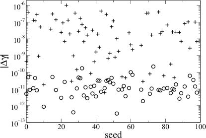
Figure 13: Deformation per cycle for all ratcheting simulations. $100$ different configurations were generated using different random number seeds.

When the Cundall-Strack algorithm is modified as described in Sec. IV.1.3, $62$ still simulations exhibit ratcheting, but at a much lower amplitude. One observes $10^{-13}<|\Delta\gamma|<2.5\times 10^{-10}$ with a geometric mean of $1.1\times 10^{-11}$. These results are summarized in Fig. 13. One sees that the use of the corrected equations leads to a $10^{4}$-fold reduction of granular ratcheting.

Figure 14: Dependence of ratcheting on time step. Crosses: original algorithm. Circles: corrected algorithm. The time step is given in multiples of $\sqrt{K/m_{\mathrm{min}}}$, where $m_{\mathrm{min}}$ is the smallest particle in the simulation.

The remaining granular ratcheting is due to integration errors. This can be shown by taking a single initial condition, and changing the time step. Typical results are shown in Fig. 14. With the original Cundall-Strack algorithm, ratcheting is independent of the time step. When it is modified, then the ratcheting deformation is proportional to the time step.

Finally, when the method described in Sec. IV.1 is implemented by direct calculation of angles, no simulations ratchet. $28$ of the simulations exhibit a constant strain with $|\gamma|<10^{-14}$ for every cycle. Note that such small deformations are not even visible on Figs. 13 and 14. The others exhibit a variety of other behaviors that will be discussed in the next section.

IV.2.3 New behaviors in small systems

Figure 15: Strain as a function of cycle number for a simulation with outliers.

Once ratcheting has been removed or reduced, new behaviors come to the foreground. The most common of these are outliers. The strain is independent of cycle number, except for occasional cycles. An example is shown in Fig. 15.

Figure 16: A configuration that causes outliers. The arrow shows the motion of the rattler. The normal forces are shown by the lines connecting particle centers. The tangential forces are shown by lines perpendicular to the normal forces. Note that the rattler does not participate in the force network.

A closer inspection of these simulations reveals that these outliers are due to “rattlers”: particles without contacts. Since there is no gravity, rattlers float inside cages in the packing. Occasionally, they collide with walls of their cage. These collisions coincide with the outlying points. Once the collision is past, the packing returns to its initial state, and the rattler floats off toward another part of its cage. The packing that produced Fig. 15 is shown in Fig. 16. The rattler is found in the upper center of the packing. It moves within a cage formed by five particles and the upper wall. The outlying points in Fig. 15 coincide with collisions between the rattler and its cage. However, not all collisions leave a trace in Fig. 15; the amplitude registered in Fig. 15 probably strongly depends on the time within the cycle where the collision takes place.

Figure 17: Accumulated strain $\gamma$ versus cycle number for a simulation performed with the angle based method of calculating tangential forces. The strain is periodic. This arises when the rattler is confined in a very small cage.

The frequency of collisions with the cage can vary widely. Sometimes only one point out of $70$ is perturbed. In other cases, every point can be considered as an outlier. Another thing that can happen when the rattler’s cage is small is that it can be driven in the cage by the motion of the surrouding particles in a periodic way. This leads to a periodic dependence of $\gamma$ on $N$, as shown in Fig. 17.

Rattler-induced outliers exist also in the original Cundall and Strack method. When on inspects the $29$ non-ratcheting simulations, one finds that $25$ of them have perturbations due to rattlers.

Another effect that rattlers can cause is a sudden step in the strain. This occurs when the particles forming the cage have only weak contact forces. The rattler can induce a sudden step in the strain by provoking a small re-arrangement of these particles.

One way to reduce the effect of the rattlers is to apply a weak gravitational field so that they can no longer float slowly from one side of their cage to another. When this is done, outliers still exist, but the perturbations they introduce are much smaller – $O(10^{-12})$ instead of $O(10^{-7})$.

Another phenomenon is “shakedown”, which has already been investigated Ramon . In “shakedown”, the accumulated strain per cycle decreases each cycle. In Fig.18, we show an example. The time required to reach a level of negligible strain accumulation is variable. In Fig. 18, strain is still accumulating, even after $1000$ cycles. In other simulations, shakedown occurs after very few simulations.

Figure 18: Accumulated strain $\gamma$ versus cycle number for a simulation performed with the angle based method of calculating tangential forces. This sample exhibits shake down.

IV.2.4 Large systems

To study these phenomena in larger systems, a series of $25$ simulations with $400$ particles was carried out. With the original Cundall–Strack method, ratcheting is observed, with a much narrower range of strain accumulation, as discussed in Sec. II.4. When either of the modifications proposed in Sec. IV.1 is used, outliers dominate the stress - cycle graphs. This is probably because as the packing becomes large, the probability of having a rattler approaches unity. When a weak gravitational field is applied, the phenomena of “shakedown” dominates.

V Conclusions

We have uncovered the cause of granular ratcheting. It is due to a potential energy that depends not only on the particle positions, but also on their past trajectories. As a granular assembly is subjected to cyclic loading, it is impossible to return both the particle positions and the contact forces to their initial values, so a small deformation occurs with each cycle. It follows that granular ratcheting can be eliminated by defining a potential energy depending only on the current particle positions. This was confirmed by extensive numerical simulations using two different implementations of this idea.

This result suggests that contact modeling should focus on the potential energy as the fundamental quantity, and then use Eq. (29) to obtain the forces. In contrast, the most common approach taken in the literature is to directly postulate forces based on physical grounds, without considering the potential energy.

One possible criticism of this work is that it is only concerned with disks, whereas ratcheting has been found in packings of polygons. The motion of disks is much simper to analyze, because the rotation of the disks is uncoupled from the translation. In polygons, this is no longer true. But all that is required is that the potential energy be path dependent. One common force law, used in granular ratcheting studies Fernando is to assume that the force between polygons is proportional to the overlap area. This force law has been shown to violate energy conservation Thorsten . Thus it seems likely that the explanation of granular ratcheting presented here also applies to ratcheting of packings of polygons.

At a detailed level, the numerical mechanism cannot be the same as the physical one. Numerical granular ratcheting is a consequence of the way the tangential spring is stretched. In experiments, the contacts between the particles are not governed by the stretching of springs. Indeed, if two touching particles can be considered as making up a single elastic body, then force and position cycles will coincide, as there is a potential energy.

However, the results of this paper do show that granular ratcheting in the experiments will occur if force and position cycles are not equal. In principle, this could be checked by examining a single contact under cyclic loading. Such an experiment would be difficult to do, since very small relative displacements must be measured. And it must also be mentioned that the idea of two contacting particles acting as if they were welded together at the contact surface is itself an idealization. There may be zones of slip at the contact (even when the contact as a whole does not slide), and this may give rise to a complicated behavior when the contact is subjected to cyclic loading. Another possibility is that fluid could coat the surfaces of the touching particles, possibly lubricating them. Or abrasion at the contact point could generate very tiny particles trapped between the two touching surfaces. These particles could act like fault gouge gouge on a very small scale, facilitating a relative tangential motion. All of these effects may lead to a history dependent potential energy, and thus to granular ratcheting through the mechanism discussed in this paper.

Appendix A Stiffness Matrix Theory

The section presents a very brief review of stiffness matrix theory. This theory applies to granular packings under quasi-static loading, and thus is applicable to granular ratcheting. We explain below how this theory explains certain key properties of packing under cyclic loading, namely,

• why particle trajectories are straight lines when there are no sliding contacts, and the forcing is given by Eq. (1),

• why this is no longer true when there are sliding contacts, and

• why the forcing given in Eq. (4) generates particle trajectories with a non-zero area.

A.1 Introduction to stiffness matrix theory

In stiffness matrix theory one , the behavior of the packing is piece-wise linear. Thus time can be divided into intervals $[t_{i},t_{i+1}]$ during which the velocities of the particles are linearly related to the change in forces:

$$\frac{d\mathbf{f}_{\mathrm{ext}}}{dt}=\mathbf{kv},$$ (32)

where $\mathbf{f}_{\mathrm{ext}}$ represents the external forces ($F_{x}$ and $F_{y}$ for the biaxial box), $\mathbf{v}$ contains the velocities of the particles and walls, and $\mathbf{k}$ is called the stiffness matrix. It relates the velocities (or displacement increments) of the particles to the change in the force exerted on each particle by its neighbors.

The motion is only piece-wise linear because the stiffness matrix $\mathbf{k}$ depends on the status (sliding or not) of each contact. Whenever a contact status changes, $\mathbf{k}$ also changes. Therefore, the times $\{t_{i}\}$ which define the intervals of linearity are the times when one or more contacts change status.

Eq. (32) holds when the forcing is quasi-static, and the particles are quasi-rigid. Quasi-static forcing means that the time scale associated with the forcing is much longer than the time the packing needs to react. Particles can be said to be quasi-rigid if their stiffness is much greater than the confining pressure. Note that these two assumptions are related: if the particles are very stiff, the speed of sound is very high, and the packing can quickly react to changes in the external load.

A.2 Application to biaxial test

If one considers a biaxial test, with the forcing given by Eq. (1), then only the entries of $\mathbf{f}_{\mathrm{ext}}$ corresponding to the walls are non-zero, because no external forces are applied to the particles. Furthermore, in Eq. (32), only those components associated with varying forces survive differentiation by time. Thus Eq. (32) becomes

$$\frac{dq}{dt}\mathbf{L}_{x}=\mathbf{kv},$$ (33)

where $\mathbf{L}_{x}$ is a vector, all of whose components are zero, except the $y$ component of the force on the upper and lower walls. All other components of $\mathbf{f}_{\mathrm{ext}}$ are either zero or constant.

One would like to invert $\mathbf{k}$ and bring it onto the left hand side of the equation. But $\mathbf{k}$ is singular because there are certain collective motions that do not change the spring lengths, and hence do not change the forces. One example is the uniform motion of all particles. They do not move relative to one other, and provoke no change in force. Let $\mathbb{B}$ be the set of all such motions. We can be sure that the left hand side of Eq. (33) is orthogonal to every member of $\mathbb{B}$, for if it were not, the packing would be unstable one .

Now define the matrix $\mathbf{\hat{k}}$ that will act like an inverse of $\mathbf{k}$. It is defined by

$$\mathbf{kx}=\mathbf{f}\mbox{ and }\mathbf{x}\perp\mathbb{B}\;\Rightarrow\;\mathbf{\hat{k}f}=\mathbf{x}.$$ (34)

This equation gives the result of applying $\mathbf{\hat{k}}$ for $3N-\dim\mathbb{B}$ linearly independent vectors. To fully determine $\mathbf{\hat{k}}$, we must say how it acts on the other $\dim\mathbb{B}$ dimensions of $\mathbb{R}^{3N}$. Let $\mathbb{F}$ be the range of $\mathbf{k}$. Then:

$$\mathbf{\hat{k}f}=0,\mbox{ for }\mathbf{f}\perp\mathbb{F}.$$ (35)

This determines $\mathbf{\hat{k}}$. Note that $\mathbf{\hat{k}k}$ is a projector that removes $\mathbb{B}$.

Using this in Eq. (33), one can write:

$$\mathbf{v}=\frac{dq}{dt}\mathbf{\hat{k}L}_{x},$$ (36)

which can be integrated:

$$\mathbf{x}=\mathbf{x}_{0}+q(t)\mathbf{\hat{k}L}_{x}.$$ (37)

Here $\mathbf{x}$ is a vector containing the positions of the particles and walls. Eq. (37 shows that the position of each particle moves back and forth on a line defined by the appropriate components of $\mathbf{\hat{k}L}_{x}$. So no area is traced out by position cycles, and ratcheting does not occur.

But if there are sliding contacts, then $\mathbf{k}$ does not remain constant. Recall that $\mathbf{k}$ changes whenever a contact changes status. Thus when a contact starts or stops sliding, the relation between $\mathbf{v}$ and $\mathbf{f}_{\mathrm{ext}}$ changes, and the particle motion changes direction. This is what we saw in Fig. 4.

Another way to get paths that are not lines is add another term to the left hand side of Eq. (33). When we use the forcing given in Eq. (4) and (5), then Eq. (33) becomes

$$\frac{dq_{x}}{dt}\mathbf{L}_{x}+\frac{dq_{y}}{dt}\mathbf{L}_{y}=\mathbf{kv},$$ (38)

and thus the motion is

$$\mathbf{x}=\mathbf{x}_{0}+q_{x}(t)\mathbf{\hat{k}L}_{x}+q_{y}(t)\mathbf{\hat{k}L}_{y}.$$ (39)

Thus if the forcing traces out an area in the $(q_{x},q_{y})$ plane, than each contact traces out a proportional area in the relative position plane. This, together with Eq. 17, explains the result in Fig. 5.