Optimal Causal Inference:
Estimating Stored Information and Approximating Causal Architecture

Abstract

We introduce an approach to inferring the causal architecture of stochastic dynamical systems that extends rate distortion theory to use causal shielding—a natural principle of learning. We study two distinct cases of causal inference: optimal causal filtering and optimal causal estimation.

Filtering corresponds to the ideal case in which the probability distribution of measurement sequences is known, giving a principled method to approximate a system’s causal structure at a desired level of representation. We show that, in the limit in which a model complexity constraint is relaxed, filtering finds the exact causal architecture of a stochastic dynamical system, known as the causal-state partition. From this, one can estimate the amount of historical information the process stores. More generally, causal filtering finds a graded model-complexity hierarchy of approximations to the causal architecture. Abrupt changes in the hierarchy, as a function of approximation, capture distinct scales of structural organization.

For nonideal cases with finite data, we show how the correct number of underlying causal states can be found by optimal causal estimation. A previously derived model complexity control term allows us to correct for the effect of statistical fluctuations in probability estimates and thereby avoid over-fitting.

Natural systems compute intrinsically and produce information. This organization, often only indirectly accessible to an observer, is reflected to varying degrees in measured time series. Nonetheless, this information can be used to build models of varying complexity that capture the causal architecture of the underlying system and allow one to estimate its information processing capabilities. We investigate two cases. The first is when a model builder wishes to find a more compact representation than the true one. This occurs, for example, when one is willing to incur the cost of a small increase in error for a large reduction in model size. The second case concerns the empirical setting in which only a finite amount of data is available. There one wishes to avoid over-fitting a model to a particular data set.

I Introduction

Time series modeling has a long and important history in science and engineering. Advances in dynamical systems over the last half century led to new methods that attempt to account for the inherent nonlinearity in many natural phenomena (Berge et al., 1986; Guckenheimer and Holmes, 1983; Wiggins, 1988; Devaney, 1989; Lieberman and Lichtenberg, 1993; Ott, 1993; Strogatz, 1994). As a result, it is now well known that nonlinear systems produce highly correlated time series that are not adequately modeled under the typical statistical assumptions of linearity, independence, and identical distributions. One consequence, exploited in novel state-space reconstruction methods (Packard et al., 1980; Takens, 1981; Fraser, 1991), is that discovering the hidden structure of such processes is key to successful modeling and prediction (Crutchfield and McNamara, 1987; Casdagli and Eubank, 1992; Sprott, 2003; Kantz and Schreiber, 2006). In an attempt to unify the alternative nonlinear modeling approaches, computational mechanics Crutchfield and Young (1989) introduced a minimal representation—the $\epsilon$-machine—for stochastic dynamical systems that is an optimal predictor and from which many system properties can be directly calculated. Building on the notion of state introduced in Ref. Packard et al. (1980), a system’s effective states are those variables that causally shield a system’s past from its future—capturing, in the present, information from the past that predicts the future.

Following these lines, here we investigate the problem of learning predictive models of time series with particular attention paid to discovering hidden variables. We do this by using the information bottleneck method (IB) (Tishby et al., 1999) together with a complexity control method discussed by Ref. (Still and Bialek, 2004), which is necessary for learning from finite data. Ref. Shalizi and Crutchfield (2002) lays out the relationship between computational mechanics and the information bottleneck method. Here, we make the mathematical connection for times series, introducing a new method.

We adapt IB to time series prediction, resulting in a method we call optimal causal filtering (OCF) . Since OCF, in effect, extends rate-distortion theory (Shannon, 1948) to use causal shielding, in general it achieves an optimal balance between model complexity and approximation accuracy. The implications of these trade-offs for automated theory building are discussed in Ref. (Still and Crutchfield, 2007).

We show that in the important limit in which prediction is paramount and model complexity is not restricted, OCF reconstructs the underlying process’s causal architecture, as previously defined within the framework of computational mechanics (Crutchfield and Young, 1989; Crutchfield, 1994; Crutchfield and Shalizi, 1999). This shows that, in effect, OCF captures a source’s hidden variables and organization. The result gives structural meaning to the inferred models. For example, one can calculate fundamental invariants—such as, symmetries, entropy rate, and stored information—of the original system.

To handle finite-data fluctuations, OCF is extended to optimal causal estimation (OCE). When probabilities are estimated from finite data, errors due to statistical fluctuations in probability estimates must be taken into account in order to avoid over-fitting. We demonstrate how OCF and OCI work on a number of example stochastic processes with known, nontrivial correlational structure.

II Causal States

Assume that we are given a stochastic process ${\rm P}(\stackrel{{\scriptstyle\leftrightarrow}}{{{X}}})$—a joint distribution over a bi-infinite sequence $\stackrel{{\scriptstyle\leftrightarrow}}{{{X}}}=\stackrel{{\scriptstyle\leftarrow}}{{{X}}}\stackrel{{\scriptstyle\rightarrow}}{{{X}}}$ of random variables. The past, or history, is denoted $\stackrel{{\scriptstyle\leftarrow}}{{{X}}}=\ldots{X}_{-3}{X}_{-2}{X}_{-1}$, while $\stackrel{{\scriptstyle\rightarrow}}{{{X}}}={X}_{0}{X}_{1}{X}_{2}\ldots$ denotes the future . Here, the random variables ${X}_{t}$ take on discrete values ${x}\in\mathcal{A}=\{1,2,\ldots,k\}$ and the process as a whole is stationary. The following assumes the reader is familiar with information theory and the notation of Ref. (Cover and Thomas, 2006).

Within computational mechanics, a process ${\rm P}(\stackrel{{\scriptstyle\leftrightarrow}}{{{X}}})$ is viewed as a communication channel that transmits information from the past to the future, storing information in the present—presumably in some internal states, variables, or degrees of freedom Crutchfield et al. (2009). One can ask a simple question, then: how much information does the past share with the future? A related and more demanding question is how we can infer a predictive model, given the process. Many authors have considered such questions. Refs. (Crutchfield and Feldman, 2003; Crutchfield and Shalizi, 1999; Shalizi and Crutchfield, 2002; Bialek et al., 2006) review some of the related literature.

The effective, or causal, states $\bm{\mathcal{S}}$ are determined by an equivalence relation ${\stackrel{{\scriptstyle\leftarrow}}{{{x}}}}\sim{\stackrel{{\scriptstyle\leftarrow}}{{{x}}}}^{\prime}$ that groups all histories together which give rise to the same prediction of the future (Crutchfield and Young, 1989; Crutchfield and Shalizi, 1999). The equivalence relation partitions the space ${\stackrel{{\scriptstyle\leftarrow}}{{\rm{\bf{X}}}}}$ of histories and is specified by the set-valued function:

$$\epsilon({\stackrel{{\scriptstyle\leftarrow}}{{{x}}}})=\{{\stackrel{{\scriptstyle\leftarrow}}{{{x}}}}^{\prime}:{\rm P}(\stackrel{{\scriptstyle\rightarrow}}{{{X}}}|{\stackrel{{\scriptstyle\leftarrow}}{{{x}}}})={\rm P}(\stackrel{{\scriptstyle\rightarrow}}{{{X}}}|{\stackrel{{\scriptstyle\leftarrow}}{{{x}}}}^{\prime})\}$$ (1)

that maps from an individual history to the equivalence class $\sigma\in\bm{\mathcal{S}}$ containing that history and all others which lead to the same prediction ${\rm P}(\stackrel{{\scriptstyle\rightarrow}}{{{X}}}|{\stackrel{{\scriptstyle\leftarrow}}{{{x}}}})$ of the future. A causal state $\sigma$ includes: (i) a label $\sigma\in\bm{\mathcal{S}}$; (ii) a set of histories $\stackrel{{\scriptstyle\leftarrow}}{{{X}}}_{\sigma}=\{{\stackrel{{\scriptstyle\leftarrow}}{{{x}}}}:{\rm P}(\stackrel{{\scriptstyle\rightarrow}}{{{X}}}|{\stackrel{{\scriptstyle\leftarrow}}{{{x}}}})={\rm P}(\stackrel{{\scriptstyle\rightarrow}}{{{X}}}|\sigma)\}\subset{\stackrel{{\scriptstyle\leftarrow}}{{\rm{\bf{X}}}}}$; and (iii) a future conditional distribution ${\rm P}(\stackrel{{\scriptstyle\rightarrow}}{{{X}}}|\sigma)$ given the state (Crutchfield and Young, 1989; Crutchfield and Shalizi, 1999).

Any alternative model, called a rival ${\cal R}$, gives a probabilistic assignment ${\rm P}({\cal R}|{\stackrel{{\scriptstyle\leftarrow}}{{{x}}}})$ of histories to its states $\rho\in\bm{{\cal R}}$. Due to the data processing inequality, a model can never capture more information about the future than shared between past and future:

$$I[{\cal R};\stackrel{{\scriptstyle\rightarrow}}{{{X}}}]\leq I[\stackrel{{\scriptstyle\leftarrow}}{{{X}}};\stackrel{{\scriptstyle\rightarrow}}{{{X}}}]~{},$$ (2)

where $I[V,W]$ denotes the mutual information between random variables $V$ and $W$ (Cover and Thomas, 2006). The quantity ${\bf E}=I[\stackrel{{\scriptstyle\leftarrow}}{{{X}}};\stackrel{{\scriptstyle\rightarrow}}{{{X}}}]$ has been studied by several authors and given different names, such as (in chronological order) convergence rate of the conditional entropy (del Junco and Rahe, 1979), excess entropy (Crutchfield and Packard, 1983), stored information Shaw (1984), effective measure complexity (Grassberger, 1986), past-future mutual information (Li, 1991), and predictive information (Bialek and Tishby, 1999), amongst others. For a review see Ref. (Crutchfield and Feldman, 2003) and references therein.

The causal states $\sigma\in\bm{\mathcal{S}}$ are distinguished by the fact that the function $\epsilon(\cdot)$ gives rise to a deterministic assignment of histories to states:

$${\rm P}(\sigma|{\stackrel{{\scriptstyle\leftarrow}}{{{x}}}})=\delta_{\sigma,\epsilon({\stackrel{{\scriptstyle\leftarrow}}{{{x}}}})}~{},$$ (3)

and, furthermore, by the fact that their future conditional probabilities are given by

$${\rm P}(\stackrel{{\scriptstyle\rightarrow}}{{{X}}}|\sigma)={\rm P}(\stackrel{{\scriptstyle\rightarrow}}{{{X}}}|{\stackrel{{\scriptstyle\leftarrow}}{{{x}}}})~{},$$ (4)

for all ${\stackrel{{\scriptstyle\leftarrow}}{{{x}}}}$ such that $\epsilon({\stackrel{{\scriptstyle\leftarrow}}{{{x}}}})=\sigma$. As a consequence, the causal states, considered as a random variable $\mathcal{S}$, capture the full predictive information

$$I[\mathcal{S};\stackrel{{\scriptstyle\rightarrow}}{{{X}}}]=I[\stackrel{{\scriptstyle\leftarrow}}{{{X}}};\stackrel{{\scriptstyle\rightarrow}}{{{X}}}]={\bf E}~{}.$$ (5)

More to the point, they causally shield the past and future—the past and future are independent given the causal state: ${\rm P}(\stackrel{{\scriptstyle\leftarrow}}{{{X}}},\stackrel{{\scriptstyle\rightarrow}}{{{X}}}|\mathcal{S})={\rm P}(\stackrel{{\scriptstyle\leftarrow}}{{{X}}}|\mathcal{S}){\rm P}(\stackrel{{\scriptstyle\rightarrow}}{{{X}}}|\mathcal{S})$.

The causal-state partition has, out of all equally predictive partitions, called prescient rivals $\widehat{{\cal R}}$ Crutchfield et al. (2010), the smallest entropy, ${C_{\mu}}[{\cal R}]=H[{\cal R}]$:

$$H[\widehat{{\cal R}}]\geq H[\mathcal{S}]~{},$$ (6)

known as the statistical complexity, ${C_{\mu}}:=H[\mathcal{S}]$. This is amount of historical information a process stores: A process communicates ${\bf E}$ bits from the past to the future by storing ${C_{\mu}}$ bits in the present. ${C_{\mu}}$ is one of a process’s key properties; the other is its entropy rate (Cover and Thomas, 2006). Finally, the causal states are unique and minimal sufficient statistics for prediction of the time series (Crutchfield and Young, 1989; Crutchfield and Shalizi, 1999).

III Constructing Causal Models of Information Sources

Continuing with the communication channel analogy above, models, optimal or not, can be broadly considered to be a lossy compression of the original data. A model captures some regularity while making some errors in describing the data. Rate distortion theory (Shannon, 1948) gives a principled method to find a lossy compression of an information source such that the resulting model is as faithful as possible to the original data, quantified by a distortion function. The specific form of the distortion function determines what is considered to be “relevant”—kept in the compressed representation—and what is “irrelevant”—can be discarded. Since there is no universal distortion function, it has to be assumed ad hoc for each application. The information bottleneck method (Tishby et al., 1999) argues for explicitly keeping the relevant information, defined as the mutual information that the data share with a desired relevant variable (Tishby et al., 1999). With those choices, the distortion function can be derived from the optimization principle, but the relevant variable has to be specified a priori.

In time series modeling, however, there is a natural notion of relevance: the future data. For stationary time series, moreover, building a model with low generalization error is equivalent to constructing a model that accurately predicts future data from past data. These observations lead directly to an information-theoretic specification for reconstructing time series models: First, introduce general model variables ${\cal R}$ that can store, in the present moment, the information transmitted from the past to the future. Any set of such variables specifies a stochastic partition of ${\stackrel{{\scriptstyle\leftarrow}}{{\rm{\bf{X}}}}}$ via a probabilistic assignment rule ${\rm P}({\cal R}|{\stackrel{{\scriptstyle\leftarrow}}{{{x}}}})$. Second, require that this partition be maximally predictive. That is, it should maximize the information $I[{\cal R};\stackrel{{\scriptstyle\rightarrow}}{{{X}}}]$ that the variables ${\cal R}$ contain about the future $\stackrel{{\scriptstyle\rightarrow}}{{{X}}}$. Third, the so-constructed representation of the historical data should be a summary, i.e., it should not contain all of the historical information, but rather, as little as possible while still capturing the predictive information. The information kept about the past—$I[\stackrel{{\scriptstyle\leftarrow}}{{{X}}};{\cal R}]$, the coding rate—measures the model complexity or bit cost. Intuitively, one wants to find the most predictive model at fixed complexity or, vice versa, the least complex model at fixed prediction accuracy. These criteria are equivalent, in effect, to causal shielding.

Writing this intuition formally reduces to the information bottleneck method, where the relevant information is information about the future. The constrained optimization problem one has to solve is:

$$\max_{{\rm P}({\cal R}|\stackrel{{\scriptstyle\leftarrow}}{{{X}}})}\left\{I[{\cal R};\stackrel{{\scriptstyle\rightarrow}}{{{X}}}]-\lambda I[\stackrel{{\scriptstyle\leftarrow}}{{{X}}};{\cal R}]\right\}~{},$$ (7)

where the parameter $\lambda$ controls the balance between prediction and model complexity. The linear trade-off that $\lambda$ represents is an ad hoc assumption Shalizi and Crutchfield (2002). Its justification is greatly strengthened in the following by the rigorous results showing it leads to the causal states and the successful quantitative applications.

The optimization problem of Eq. (7) is solved subject to the normalization constraint: $\sum_{\cal R}{\rm P}({\cal R}|{\stackrel{{\scriptstyle\leftarrow}}{{{x}}}})=1$, for all ${\stackrel{{\scriptstyle\leftarrow}}{{{x}}}}\in{\stackrel{{\scriptstyle\leftarrow}}{{\rm{\bf{X}}}}}$. It then has a family of solutions (Tishby et al., 1999), parametrized by the Lagrange multiplier $\lambda$, that gives the following optimal assignments of histories ${\stackrel{{\scriptstyle\leftarrow}}{{{x}}}}$ to states $\rho\in{\cal R}$:

$${\rm P}_{\mathrm{opt}}(\rho|{\stackrel{{\scriptstyle\leftarrow}}{{{x}}}})=\frac{{\rm P}(\rho)}{Z({\stackrel{{\scriptstyle\leftarrow}}{{{x}}}},\lambda)}\exp{\left(-\frac{1}{\lambda}\mathcal{D}\left({{\rm P}(\stackrel{{\scriptstyle\rightarrow}}{{{X}}}|{\stackrel{{\scriptstyle\leftarrow}}{{{x}}}})}||{{\rm P}(\stackrel{{\scriptstyle\rightarrow}}{{{X}}}|\rho)}\right)\right),}$$ (8)

with

$${\rm P}(\stackrel{{\scriptstyle\rightarrow}}{{{X}}}|\rho) = \frac{1}{{\rm P}(\rho)}\sum_{{\stackrel{{\scriptstyle\leftarrow}}{{{x}}}}\in{\stackrel{{\scriptstyle\leftarrow}}{{\rm{\bf{X}}}}}}{\rm P}(\stackrel{{\scriptstyle\rightarrow}}{{{X}}}|{\stackrel{{\scriptstyle\leftarrow}}{{{x}}}}){\rm P}(\rho|{\stackrel{{\scriptstyle\leftarrow}}{{{x}}}}){\rm P}({\stackrel{{\scriptstyle\leftarrow}}{{{x}}}})~{}\mathrm{and}$$ (9)

$${\rm P}(\rho) = \sum_{{\stackrel{{\scriptstyle\leftarrow}}{{{x}}}}\in{\stackrel{{\scriptstyle\leftarrow}}{{\rm{\bf{X}}}}}}{\rm P}(\rho|{\stackrel{{\scriptstyle\leftarrow}}{{{x}}}}){\rm P}({\stackrel{{\scriptstyle\leftarrow}}{{{x}}}})~{},$$ (10)

where $\mathcal{D}\left({P}||{Q}\right)$ is the information gain (Cover and Thomas, 2006) between distributions $P$ and $Q$. In the solution it plays the role of an “energy”, effectively measuring how different the predicted and true futures are. The more distinct, the more information one gains about the probabilistic development of the future from the past. That is, high energy models make predictions that deviate substantially from the process.

These self-consistent equations are solved iteratively (Tishby et al., 1999) using a procedure similar to the Blahut-Arimoto algorithm (Arimoto, 1972; Blahut, 1972). A connection to statistical mechanics is often drawn, and the parameter $\lambda$ is identified with a (pseudo) temperature that controls the level of randomness; see, e.g., Ref. (Rose et al., 1990). This is useful to guide intuition and, for example, has inspired deterministic annealing (Rose, 1998).

We are now ready for the first observation.

Proposition 1.

In the low-temperature regime ($\lambda\rightarrow 0$) the assignments of pasts to states become deterministic and are given by:

$${\rm P}_{\mathrm{opt}}(\rho|{\stackrel{{\scriptstyle\leftarrow}}{{{x}}}}) = \delta_{\rho,\eta({\stackrel{{\scriptstyle\leftarrow}}{{{x}}}})}~{},~{}\mathrm{where}$$ (11)

$$\eta({\stackrel{{\scriptstyle\leftarrow}}{{{x}}}}) = {\rm arg}\min_{\rho}\mathcal{D}\left({{\rm P}(\stackrel{{\scriptstyle\rightarrow}}{{{X}}}|{\stackrel{{\scriptstyle\leftarrow}}{{{x}}}})}||{{\rm P}(\stackrel{{\scriptstyle\rightarrow}}{{{X}}}|\rho)}\right)~{}.$$ (12)

Proof.

Define the quantity

$$D(\rho)= \mathcal{D}\left({{\rm P}(\stackrel{{\scriptstyle\rightarrow}}{{{X}}}|{\stackrel{{\scriptstyle\leftarrow}}{{{x}}}})}||{{\rm P}(\stackrel{{\scriptstyle\rightarrow}}{{{X}}}|\rho)}\right)$$

$$-\mathcal{D}\left({{\rm P}(\stackrel{{\scriptstyle\rightarrow}}{{{X}}}|{\stackrel{{\scriptstyle\leftarrow}}{{{x}}}})}||{{\rm P}(\stackrel{{\scriptstyle\rightarrow}}{{{X}}}|\eta({\stackrel{{\scriptstyle\leftarrow}}{{{x}}}}))}\right)~{}.$$ (13)

$D(\rho)$ is positive, by definition Eq. (12) of $\eta({\stackrel{{\scriptstyle\leftarrow}}{{{x}}}})$. Now, write

$${\rm P}_{\mathrm{opt}}(\eta({\stackrel{{\scriptstyle\leftarrow}}{{{x}}}})|{\stackrel{{\scriptstyle\leftarrow}}{{{x}}}})=\left(1+\sum_{\rho\neq\eta({\stackrel{{\scriptstyle\leftarrow}}{{{x}}}})}\frac{{\rm P}(\rho)}{{\rm P}(\eta({\stackrel{{\scriptstyle\leftarrow}}{{{x}}}}))}\exp{\left[-\frac{D(\rho)}{\lambda}\right]}\right)^{-1}.$$ (14)

The sum in the r.h.s. tends to zero, as $\lambda\rightarrow 0$, assuming that ${\rm P}(\eta({\stackrel{{\scriptstyle\leftarrow}}{{{x}}}}))>0$. Via normalization, the assignments become deterministic. ∎

IV Optimal Causal Filtering

We now establish the procedure’s fundamental properties by connecting the solutions it determines to the causal representations defined previously within the framework of computational mechanics. The resulting procedure transforms the original data to a causal representation and so we call it optimal causal filtering (OCF).

Note first that for deterministic assignments we have $H[{\cal R}|\stackrel{{\scriptstyle\leftarrow}}{{{X}}}]=0$. Therefore, the information about the past becomes $I[\stackrel{{\scriptstyle\leftarrow}}{{{X}}};{\cal R}]=H[{\cal R}]$ and the objective function simplifies to

$$F_{\rm det}[{\cal R}]=I[{\cal R};\stackrel{{\scriptstyle\rightarrow}}{{{X}}}]-\lambda H[{\cal R}]~{}.$$ (15)

Lemma 1.

Within the subspace of prescient rivals, the causal-state partition maximizes $F_{\rm det}[\widehat{{\cal R}}]$.

Proof.

This follows immediately from Eqs. (5) and (6). They imply that

$$F_{\rm det}[\widehat{{\cal R}}] = I[\mathcal{S};\stackrel{{\scriptstyle\rightarrow}}{{{X}}}]-\lambda H[\widehat{{\cal R}}]$$ (16)

$$\leq I[\mathcal{S};\stackrel{{\scriptstyle\rightarrow}}{{{X}}}]-\lambda H[\mathcal{S}]$$

$$= F_{\rm det}[\mathcal{S}]~{}.$$

∎

The causal-state partition is the model with the largest value of the OCF objective function, because it is fully predictive at minimum complexity. We also know from Prop. 1 that in the low-temperature limit ($\lambda\rightarrow 0$) OCF recovers a deterministic mapping of histories to states. We now show that this mapping is exactly the causal-state partition of histories.

Theorem 1.

OCF finds the causal-state partition of ${\stackrel{{\scriptstyle\leftarrow}}{{\rm{\bf{X}}}}}$ in the low-temperature limit, $\lambda\rightarrow 0$.

Proof.

The causal-state partition, Eq. (1), always exists, and implies that there are groups of histories with

$${\rm P}(\stackrel{{\scriptstyle\rightarrow}}{{{X}}}|{\stackrel{{\scriptstyle\leftarrow}}{{{x}}}})={\rm P}(\stackrel{{\scriptstyle\rightarrow}}{{{X}}}|\epsilon({\stackrel{{\scriptstyle\leftarrow}}{{{x}}}}))~{}.$$ (17)

We then have, for all ${\stackrel{{\scriptstyle\leftarrow}}{{{x}}}}\in\stackrel{{\scriptstyle\leftarrow}}{{{X}}}$,

$$\mathcal{D}\left({{\rm P}(\stackrel{{\scriptstyle\rightarrow}}{{{X}}}|{\stackrel{{\scriptstyle\leftarrow}}{{{x}}}})}||{{\rm P}(\stackrel{{\scriptstyle\rightarrow}}{{{X}}}|\epsilon({\stackrel{{\scriptstyle\leftarrow}}{{{x}}}})}\right)=0~{},$$ (18)

and, hence,

$$\epsilon({\stackrel{{\scriptstyle\leftarrow}}{{{x}}}})={\rm arg}\min_{\rho}\mathcal{D}\left({{\rm P}(\stackrel{{\scriptstyle\rightarrow}}{{{X}}}|{\stackrel{{\scriptstyle\leftarrow}}{{{x}}}})}||{{\rm P}(\stackrel{{\scriptstyle\rightarrow}}{{{X}}}|\rho)}\right)~{}.$$ (19)

Therefore, we can identify $\epsilon({\stackrel{{\scriptstyle\leftarrow}}{{{x}}}})=\eta({\stackrel{{\scriptstyle\leftarrow}}{{{x}}}})$ in Eq. (12), and so the assignment of histories to the causal states is recovered by OCF:

$${\rm P}_{\rm opt}(\rho|{\stackrel{{\scriptstyle\leftarrow}}{{{x}}}})=\delta_{\rho,\epsilon({\stackrel{{\scriptstyle\leftarrow}}{{{x}}}})}~{}.$$ (20)

∎

Note that we have not restricted the size of the set $\bm{{\cal R}}$ of model states. Recall also that the causal-state partition is unique (Crutchfield and Shalizi, 1999). The Lemma establishes that OCF does not find prescient rivals in the low-temperature limit. The prescient rivals are suboptimal in the particular sense that they have smaller values of the objective function. We now establish that this difference is controlled by the model size with proportionality constant $\lambda$.

Corollary 1.

Prescient rivals are suboptimal in OCF. The value of the objective function evaluated for a prescient rival is smaller than that evaluated for the causal-state model. The difference $\Delta F_{\rm det}[\widehat{{\cal R}}]=F_{\rm det}[\mathcal{S}]-F_{\rm det}[\widehat{{\cal R}}]$ is given by:

$$\Delta F_{\rm det}[\widehat{{\cal R}}]=\lambda\left({C_{\mu}}[\widehat{{\cal R}}]-{C_{\mu}}[\mathcal{S}]\right)\geq 0~{}.$$ (21)

Proof.

$$\Delta F_{\rm det}[\widehat{{\cal R}}] =F_{\rm det}[\mathcal{S}]-F_{\rm det}[\widehat{{\cal R}}]$$ (22)

$$=I[\mathcal{S};\stackrel{{\scriptstyle\rightarrow}}{{{X}}}]-I[\widehat{{\cal R}};\stackrel{{\scriptstyle\rightarrow}}{{{X}}}]-\lambda H[\mathcal{S}]+\lambda H[\widehat{{\cal R}}]$$ (23)

$$=\lambda\left({C_{\mu}}[\widehat{{\cal R}}]-{C_{\mu}}[\mathcal{S}]\right)~{}.$$ (24)

Moreover, Eq. (6) implies that $\Delta F_{\rm det}\geq 0$. ∎

So, we see that for $\lambda=0$, causal states and all other prescient rival partitions are degenerate. This is to be expected as at $\lambda=0$ the model-complexity constraint disappears. Importantly, this means that maximizing the predictive information alone, without the appropriate constraint on model complexity does not suffice to recover the causal-state partition.

V Examples

We study how OCF works on a series of example stochastic processes of increasing statistical sophistication. We compute the optimal solutions and visualize the trade-off between predictive power and complexity of the model by tracing out a curve similar to a rate-distortion curve (Arimoto, 1972; Blahut, 1972): For each value of $\lambda$, we evaluate both the model’s coding rate $I[\stackrel{{\scriptstyle\leftarrow}}{{{X}}};{\cal R}]$ and its predicted information $I[{\cal R};\stackrel{{\scriptstyle\rightarrow}}{{{X}}}]$ at the optimal solution and plot them against each other. The resulting curve in the information plane (Tishby et al., 1999) separates the feasible from the infeasible region: It is possible to find a model that is more complex at the same prediction error, but not possible to find a less complex model than that given by the optimum. In analogy to a rate-distortion curve, we can read off the maximum amount of information about the future that can be captured with a model of fixed complexity. Or, conversely, we can read off the smallest representation at fixed predictive power.

The examples in this and the following sections are calculated by solving the self-consistent Eqs. (8) to (10) iteratively at each value of $\lambda$. To trace out the curves, a deterministic annealing (Rose, 1998) scheme is implemented, lowering $\lambda$ by a fixed annealing rate. Smaller rates cost more computational time, but allow one to compute the rate-distortion curve in greater detail, while larger rates result in a rate-distortion curve that gets evaluated in fewer places and hence looks coarser. In examples, naturally, one can only work with finite length past and future sequences: $\stackrel{{\scriptstyle\leftarrow}}{{{x}}}\stackrel{{\scriptstyle{K}}}{{}}$ and $\stackrel{{\scriptstyle\rightarrow}}{{{x}}}\stackrel{{\scriptstyle{L}}}{{}}$, where $K$ and $L$ give their lengths, respectively.

V.1 Periodic limit cycle: A predictable process

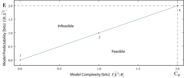
Figure 1: Model predictability $I[{\cal R};\stackrel{{\scriptstyle\rightarrow}}{{{X}}}\stackrel{{\scriptstyle{L}}}{{}}]$ versus model complexity (size) $I[\stackrel{{\scriptstyle\leftarrow}}{{{X}}}\stackrel{{\scriptstyle{K}}}{{}};{\cal R}]$ trade-off under OCF for the exactly predictable period-$4$ process: $(0011)^{\infty}$. Monitored in the information plane. The horizontal dashed line is the full predictive information (${\bf E}=I[\stackrel{{\scriptstyle\leftarrow}}{{{X}}}\stackrel{{\scriptstyle{3}}}{{}};\stackrel{{\scriptstyle\rightarrow}}{{{X}}}\stackrel{{\scriptstyle{2}}}{{}}]=2$ bits) and the vertical dashed line is the block entropy ($H[\stackrel{{\scriptstyle\leftarrow}}{{{X}}}\stackrel{{\scriptstyle{3}}}{{}}]=2$ bits), which is also the statistical complexity ${C_{\mu}}$. The data points represent solutions at various $\lambda$. Lines connect them to help guide the eye only. Histories of length $K=3$ were used, along with futures of length $L=2$. In this and the following information plane plots, the integer labels $N_{c}$ indicate the first point at which the effective number of states used by the model equals $N_{c}$.

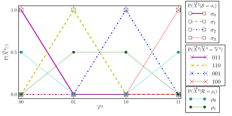
Figure 2: Morphs ${\rm P}(\stackrel{{\scriptstyle\rightarrow}}{{{X}}}\stackrel{{\scriptstyle{2}}}{{}}|\cdot)$ for the period-$4$ process: The $2$-state approximation (circles) compared to the $\delta$-function morphs for the $4$ causal states (boxes). The morphs ${\rm P}(\stackrel{{\scriptstyle\rightarrow}}{{{X}}}\stackrel{{\scriptstyle{2}}}{{}}|\sigma)$ for the two-state approximation are $(1/2,0,0,1/2)$ and $(0,1/2,1/2,0)$ and for the four-state case $(1,0,0,0)$, $(0,1,0,0)$, $(0,0,1,0)$, and $(0,0,0,1)$. Histories of length $K=3$ were used, along with futures of length $L=2$ (crosses).

We start with an example of an exactly periodic process, a limit cycle oscillation. It falls in the class of deterministic and time reversible processes, for which the rate-distortion curve can be computed analytically—it lies on the diagonal (Still and Crutchfield, 2007). We demonstrate this with a numerical example. Figure 1 shows how OCF works on a period-four process: $(0011)^{\infty}$. (See Figs. 1 and 2.) There are exactly two bits of predictive information $I[\stackrel{{\scriptstyle\leftarrow}}{{{X}}};\stackrel{{\scriptstyle\rightarrow}}{{{X}}}]$ to be captured about future words of length two (dotted horizontal line). This information describes the phase of the period-four cycle. To capture those two bits, one needs exactly four underlying causal states and a model complexity of ${C_{\mu}}=2$ bits (dotted vertical line).

The curve is the analog of a rate-distortion curve, except that the information plane swaps the horizontal and vertical axes—the coding rate and distortion axes. (See Ref. (Still and Crutchfield, 2007) for the direct use of the rate-distortion curve.) The value of $I[{\cal R};\stackrel{{\scriptstyle\rightarrow}}{{{X}}}\stackrel{{\scriptstyle{2}}}{{}}]$ (the “distortion”), evaluated at the optimal distribution, Eq. (8), is plotted versus $I[\stackrel{{\scriptstyle\leftarrow}}{{{X}}}\stackrel{{\scriptstyle{3}}}{{}};{\cal R}]$ (the “code rate”), also evaluated at the optimum. Those are plotted for different values of $\lambda$ and, to trace out the curve, deterministic annealing is implemented. At large $\lambda$, we are in the lower left of the curve—the compression is extreme, but no predictive information is captured. A single state model, a fair coin, is found as expected. As $\lambda$ decreases (moving to the right), the next distinct point on the curve is for a two-state model, which discards half of the information. This comes exactly at the cost of one predictive bit. Finally, OCF finds a four-state model that captures all of the predictive information at no compression. The numbers next to the curve indicate the first time that the effective number of states increases to that value.

The four-state model captures the two bits of predictive information. But compressed to one bit (using two states), one can only capture one bit of predictive information. The information curve falls onto the diagonal—a straight line that is the worst case for possible beneficial trade-offs between prediction error and model complexity (Still and Crutchfield, 2007).

In Fig. 2, we show the best two-state model compared to the full (exact) four-state model. One of the future conditional probabilities captures zero probability events of “odd” $\{01,10\}$ words, assigning equal probability to the “even” $\{00,11\}$ words. The other one captures zero probability events of even words, assigning equal probability to the odd words. This captures the fundamental determinism of the process: an odd word never follows an even word and vice versa. The overall result illustrates how the actual long-range correlation in the completely predictable period-$4$ sequence is represented by a smaller stochastic model. While in the four-state model the future conditional probabilities are $\delta$-functions, in the two-state approximate model they are mixtures of those $\delta$-functions. In this way, OCF converts structure to randomness when approximating underlying states with a compressed model; cf. the analogous trade-off discussed in Ref. (Crutchfield and Feldman, 2003).

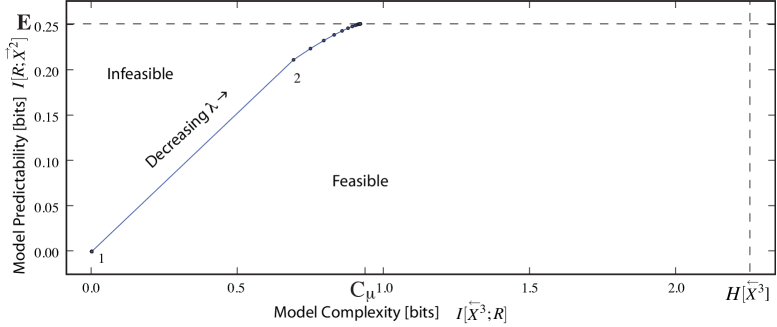
Figure 3: OCF’s behavior monitored in the information plane—$I[{\cal R};\stackrel{{\scriptstyle\rightarrow}}{{{X}}}\stackrel{{\scriptstyle{2}}}{{}}]$ versus $I[\stackrel{{\scriptstyle\leftarrow}}{{{X}}}\stackrel{{\scriptstyle{3}}}{{}};{\cal R}]$—for the Golden Mean Process. The correct two-state model is found. Histories of length $K=3$ were used, along with futures of length $L=2$. The horizontal dashed line is the full predictive information ${\bf E}\approx I[\stackrel{{\scriptstyle\leftarrow}}{{{X}}}\stackrel{{\scriptstyle{3}}}{{}};\stackrel{{\scriptstyle\rightarrow}}{{{X}}}\stackrel{{\scriptstyle{2}}}{{}}]=I[\mathcal{S};\stackrel{{\scriptstyle\rightarrow}}{{{X}}}\stackrel{{\scriptstyle{2}}}{{}}]\approx 0.25$ bits which, as seen, is an upper bound on $I[{\cal R};\stackrel{{\scriptstyle\rightarrow}}{{{X}}}\stackrel{{\scriptstyle{2}}}{{}}]$. The exact value is ${\bf E}=I[\stackrel{{\scriptstyle\leftarrow}}{{{X}}};\stackrel{{\scriptstyle\rightarrow}}{{{X}}}]=0.2516$ bits Ellison et al. (2009). Similarly, the vertical dashed line is the block entropy $H[\stackrel{{\scriptstyle\leftarrow}}{{{X}}}\stackrel{{\scriptstyle{3}}}{{}}]\approx 2.25$ bits which is an upper bound on the retrodictive information $I[\stackrel{{\scriptstyle\leftarrow}}{{{X}}}\stackrel{{\scriptstyle{3}}}{{}};{\cal R}]$. The statistical complexity ${C_{\mu}}\approx 0.92$ bits, also an upper bound, is labeled. The annealing rate was $0.952$.

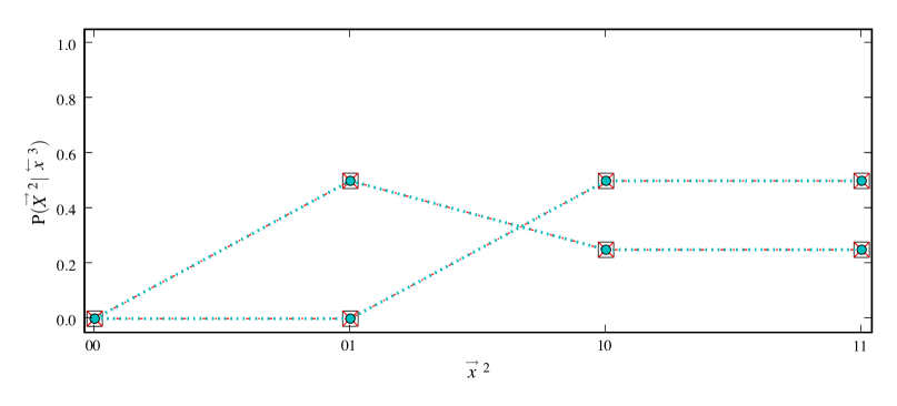
Figure 4: Future conditional probabilities ${\rm P}(\stackrel{{\scriptstyle\rightarrow}}{{{X}}}\stackrel{{\scriptstyle{2}}}{{}}|\cdot)$ conditioned on causal states $\sigma\in\bm{\mathcal{S}}$ (boxes) and on the OCF reconstructed states $\rho\in\bm{{\cal R}}$ (circles) for the Golden Mean Process. As an input to OCF, future conditional probabilities $P(\stackrel{{\scriptstyle\rightarrow}}{{{X}}}\stackrel{{\scriptstyle{2}}}{{}}|\stackrel{{\scriptstyle\leftarrow}}{{{x}}}\stackrel{{\scriptstyle{3}}}{{}})$ calculated from histories of length $K=3$ were used (crosses).

V.2 Golden Mean Process: A Markov chain

The Golden Mean (GM) Process is a Markov chain of order one. As an information source, it produces all binary strings with the restriction that there are never consecutive $0$s. The GM Process generates $0$s and $1$s with equal probability, except that once a $0$ is generated, a $1$ is always generated next. One can write down a simple two-state Markov chain for this process; see, e.g., Ref. (Crutchfield and Feldman, 2003).

Figures 3 and 4 demonstrate how OCF reconstructs the states of the GM process. Figure 3 shows the behavior of OCF in the information plane. At very high temperature ($\lambda\rightarrow\infty$, lower left corner of the curve) compression dominates over prediction and the resulting model is most compact, with only one effective causal state. However, it contains no information about the future and so is a poor predictor. As $\lambda$ decreases (moving right), OCF reconstructs increasingly more predictive and more complex models. The curve shows that the information about the future, contained in the optimal partition, increases (along the vertical axis) as the model increases in complexity (along the horizontal axis). There is a transition to two effective states: the number $2$ along the curve denotes the first occurrence of this increase. As $\lambda\rightarrow 0$, prediction comes to dominate and OCF finds a fully predictive model, albeit one with the minimal statistical complexity, out of all possible state partitions that would retain the full predictive information. The model’s complexity—${C_{\mu}}\approx 0.92$ bits—is 41% of the maximum, which is given by the entropy of all possible pasts of length $3$: $H[\stackrel{{\scriptstyle\leftarrow}}{{{X}}}\stackrel{{\scriptstyle{3}}}{{}}]\approx 2.25$ bits. The remainder (59%) of the information is nonpredictive and has been filtered out by OCF. Figure 4 shows the future conditional probabilities, associated with the partition found by OCF, as $\lambda\rightarrow 0$, corresponding to ${\rm P}(\stackrel{{\scriptstyle\rightarrow}}{{{X}}}\stackrel{{\scriptstyle{2}}}{{}}|\rho)$ (circles). These future conditional probabilities overlap with the true (but not known to the algorithm) causal-state future conditional probabilities ${\rm P}(\stackrel{{\scriptstyle\rightarrow}}{{{X}}}\stackrel{{\scriptstyle{2}}}{{}}|\sigma)$ (boxes) and so demonstrate that OCF finds the causal-state partition.

V.3 Even Process: A hidden Markov chain

Now, consider a hidden Markov process: the Even Process (Crutchfield and Feldman, 2003), which is a stochastic process whose support (the set of allowed sequences) is a symbolic dynamical system called the Even system. The Even system generates all binary strings consisting of blocks of an even number of $1$s bounded by $0$s. Having observed a process’s sequences, we say that a word (finite sequence of symbols) is forbidden if it never occurs. A word is an irreducible forbidden word if it contains no proper subwords which are themselves forbidden words. A system is sofic if its list of irreducible forbidden words is infinite. The Even system is one such sofic system, since its set $\mathcal{F}$ of irreducible forbidden words is infinite: $\mathcal{F}=\{01^{2n+1}0,n=0,1,\ldots\}$. Note that no finite-order Markovian source can generate this or, for that matter, any other strictly sofic system (Crutchfield and Feldman, 2003). The Even Process then associates probabilities with each of the Even system’s sequences by choosing a $0$ or $1$ with fair probability after generating either a $0$ or a pair of $1$s. The result is a measure sofic process—a distribution over a sofic system’s sequences.

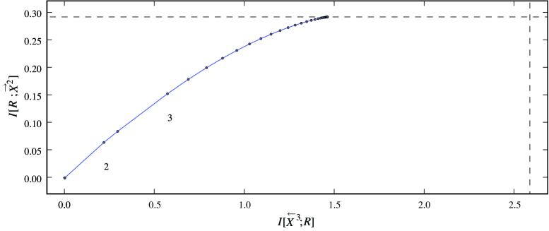
Figure 5: OCF’s behavior inferring the Even Process: monitored in the information plane—$I[{\cal R};\stackrel{{\scriptstyle\rightarrow}}{{{X}}}\stackrel{{\scriptstyle{2}}}{{}}]$ versus $I[\stackrel{{\scriptstyle\leftarrow}}{{{X}}}\stackrel{{\scriptstyle{3}}}{{}};{\cal R}]$. Histories of length $K=3$ were used, along with futures of length $L=2$. The horizontal dashed line is the full predictive information $I[\stackrel{{\scriptstyle\leftarrow}}{{{X}}}\stackrel{{\scriptstyle{3}}}{{}};\stackrel{{\scriptstyle\rightarrow}}{{{X}}}\stackrel{{\scriptstyle{2}}}{{}}]\approx 0.292$ bits which, as seen, is an upper bound on the estimates $I[{\cal R};\stackrel{{\scriptstyle\rightarrow}}{{{X}}}\stackrel{{\scriptstyle{2}}}{{}}]$. Similarly, the vertical dashed line is the block entropy $H[\stackrel{{\scriptstyle\leftarrow}}{{{X}}}\stackrel{{\scriptstyle{3}}}{{}}]\approx 2.585$ bits which is an upper bound on the retrodictive information $I[\stackrel{{\scriptstyle\leftarrow}}{{{X}}}\stackrel{{\scriptstyle{3}}}{{}};{\cal R}]$.

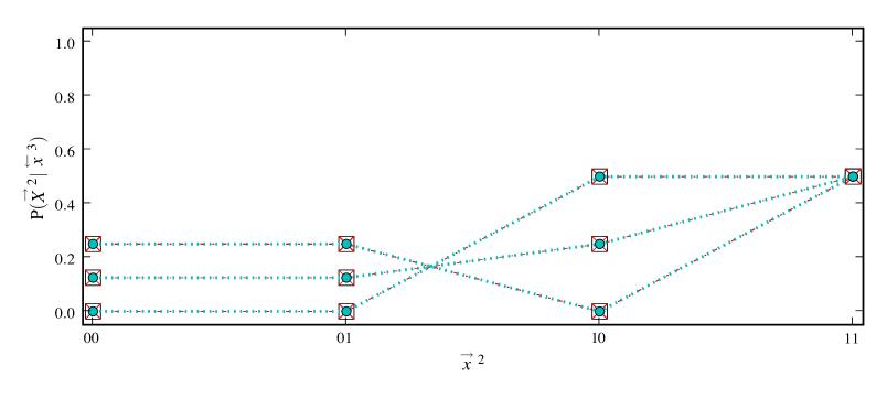
Figure 6: Future future conditional probabilities ${\rm P}(\stackrel{{\scriptstyle\rightarrow}}{{{X}}}\stackrel{{\scriptstyle{2}}}{{}}|\cdot)$ conditioned on causal states $\sigma\in\mathcal{S}$ (boxes) and on the OCF-reconstructed states $\rho\in{\cal R}$ (circles) for the Even Process. As an input to OCF, future conditional probabilities $P(\stackrel{{\scriptstyle\rightarrow}}{{{X}}}\stackrel{{\scriptstyle{2}}}{{}}|\stackrel{{\scriptstyle\leftarrow}}{{{x}}}\stackrel{{\scriptstyle{3}}}{{}})$ calculated from histories of length $K=3$ were used (crosses).

As in the previous example, for large $\lambda$, OCF applied to the Even Process recovers a small, one-state model with poor predictive quality; see Fig. 5. As $\lambda$ decreases there are transitions to larger models that capture increasingly more information about the future. (The numbers along the curve again indicate the points of first transition to more states.) With a three-state model OCF captures the full predictive information at a model size of 56% of the maximum. This model is exactly the causal-state partition, as can be seen in Fig. 6 by comparing the future conditional probabilities of the OCF model (circles) to the true underlying causal states (boxes), which are not known to the algorithm.

The correct $\epsilon$-machine model of the Even Process has four causal states: two transient and two recurrent. At the finite past and future lengths used here, OCF picks up only one of the transient states and the two recurrent states. It also assigns probability to all three. This increases the effective state entropy ($H[{\cal R}]\approx 1.48$ bits) above the statistical complexity (${C_{\mu}}=0.92$ bits) which is only a function of the two recurrent states, since asymptotically ($K\rightarrow\infty$) the transient states have zero probability.

There is an important lesson in this example for general time-series modeling, not just OCF. Correct inference of even finite-state, but measure-sofic processes requires using hidden Markov models. Related consequences of this, and one resolution, are discussed at some length for estimating “nonhidden” Markov models of sofic processes in Ref. Strelioff et al. (2007).

V.4 Random Random XOR: A structurally complex process

The previous examples demonstrated our main theoretical result: In the limit in which it becomes crucial to make the prediction error very small, at the expense of the model size, the OCF algorithm captures all of the structure inherent in the process by recovering the causal-state partition.

However, if we allow (or prefer) a model with some finite prediction error, then we can make the model substantially smaller. We have already seen what happens in the worst case scenario, for a periodic process. There, each predictive bit costs exactly one bit in terms of model size. However, for highly structured processes, there exist situations in which one can compress the model substantially at essentially no loss in terms of predictive power. (This is called causal compressibility (Still and Crutchfield, 2007).) The Even Process is an example of such an information source: The statistical complexity $H[\mathcal{S}]$ of the causal-state partition is smaller than the total available historical information—the entropy of the past $H[\stackrel{{\scriptstyle\leftarrow}}{{{X}}}\stackrel{{\scriptstyle{K}}}{{}}]$.

Now, we study a process that requires keeping all of the historical information to be maximally predictive, which is the same as stating ${C_{\mu}}({\cal R})=H[\stackrel{{\scriptstyle\leftarrow}}{{{X}}}\stackrel{{\scriptstyle{K}}}{{}}]$. (Precisely, we mean given the finite past and future lengths we use.) Nonetheless, there is a systematic ordering of models of different size and different predictive power given by the rate-distortion curve, as we change the parameter $\lambda$ that controls how much of the future fluctuations the model considers to be random; i.e., which fluctuations are considered indistinguishable. Naturally, the trade-off, and therefore the shape of the rate-distortion curve, depends on and reflects the source’s organization.

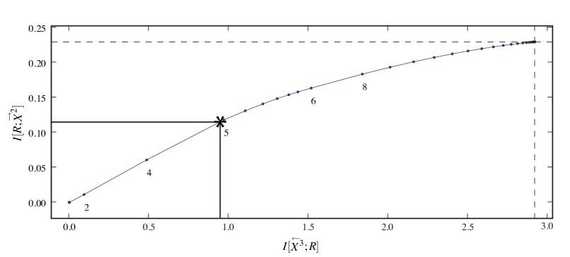
Figure 7: Prediction versus structure trade-off under OCF for the random-random XOR (RRXOR) process, as monitored in the information plane. As above, the horizontal dashed line is the predictive information ($\approx 0.230$ bits) and the vertical dashed line is the block entropy ($\approx 2.981$ bits). Histories of length $K=3$ were used, along with futures of length $L=2$. The asterisk and lines correspond to the text: they serve to show how the predictive power and the complexity of the best four state model, the future conditional probabilities of which are depicted in Fig. 9.

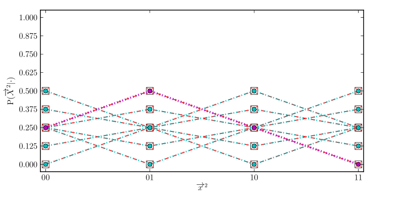
Figure 8: Future conditional probabilities ${\rm P}(\stackrel{{\scriptstyle\rightarrow}}{{{X}}}\stackrel{{\scriptstyle{2}}}{{}}|\cdot)$ for the RRXOR process: the $8$-state approximation (circles) finds the causal states (boxes). For example, the heavier dashed line (purple) shows ${\rm P}(\stackrel{{\scriptstyle\rightarrow}}{{{X}}}\stackrel{{\scriptstyle{2}}}{{}}|\rho)=(1/4,1/2,1/4,0)$. Histories of length $K=3$ were used, along with futures of length $L=2$.

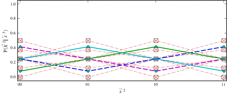
Figure 9: Morphs ${\rm P}(\stackrel{{\scriptstyle\rightarrow}}{{{X}}}\stackrel{{\scriptstyle{2}}}{{}}|\cdot)$ for the RRXOR process: the $4$-state approximation (circles and colored lines: state 1 - cyan/full, 2 - green/full, 3 - blue/dashed, 4 - purple/dashed) compared to causal states (boxes). Histories of length $K=3$ were used, along with futures of length $L=2$.

As an example, consider the random-random XOR (RRXOR) process which consists of two successive random symbols chosen to be $0$ or $1$ with equal probability and a third symbol that is the logical Exclusive-OR (XOR) of the two previous. The RRXOR process can be represented by a hidden Markov chain with five recurrent causal states, but having a very large total number of causal states. There are $36$ causal states, most ($31$) of which describe a complicated transient structure (Crutchfield and Feldman, 2003). As such, it is a structurally complex process that an analyst may wish to approximate with a smaller set of states.

Figure 7 shows the information plane, which specifies how OCF trades off structure for prediction error as a function of model complexity for the RRXOR process. The number of effective states (again first occurrences are denoted by integers along the curve) increases with model complexity. At a history length of $K=3$ and future length of $L=2$, the process has eight underlying causal states, which are found by OCF in the $\lambda\rightarrow 0$ limit. The corresponding future conditional probability distributions are shown in Fig. 8.

The RRXOR process has a structure that does not allow for substantial compression. Fig. 7 shows that the effective statistical complexity of the causal-state partition is equal to the full entropy of the past: ${C_{\mu}}({\cal R})=H[\stackrel{{\scriptstyle\leftarrow}}{{{X}}}\stackrel{{\scriptstyle{3}}}{{}}]$. So, at $L=3$, unlike the Even and Golden Mean Processes, the RRXOR process is not compressible. With half (4) of the number of states, however, OCF reconstructs a model that is only 33% as large, while capturing 50% of the information about the future. The corresponding conditional future probabilities of the (best) four-state model are shown in Fig. 9. They are mixtures of pairs of the eight causal states.

The rate-distortion curve informs the modeler about the (best possible) efficiency of predictive power to model complexity: $I[{\cal R};\stackrel{{\scriptstyle\rightarrow}}{{{X}}}]/I[\stackrel{{\scriptstyle\leftarrow}}{{{X}}};{\cal R}]$. This is useful, for example, if there are constraints on the maximum model size or, vice versa, on the minimum prediction error. For example, if we require a model of RRXOR to be 90% informative about the future, then we can read off the curve that this can be achieved at 70% of the model complexity. Generally, as $\lambda$ decreases, phase transitions occur to models with a larger number of effective states (Rose, 1998).

VI Optimal Causal Estimation: Finite-data fluctuations

In real world applications, we do not know a process’s underlying probability density, but instead must estimate it from a finite time series that we are given. Let that time series be of length $T$ and let us estimate the joint distribution of pasts (of length $K$) and futures (of length $L$) via a histogram calculated using a sliding window. Altogether we have $M=T-(K+L-1)$ observations. The resulting estimate $\widehat{{\rm P}}(\stackrel{{\scriptstyle\leftarrow}}{{{X}}}\stackrel{{\scriptstyle{K}}}{{}};\stackrel{{\scriptstyle\rightarrow}}{{{X}}}\stackrel{{\scriptstyle{L}}}{{}})$ will deviate from the true ${\rm P}(\stackrel{{\scriptstyle\leftarrow}}{{{X}}}\stackrel{{\scriptstyle{K}}}{{}};\stackrel{{\scriptstyle\rightarrow}}{{{X}}}\stackrel{{\scriptstyle{L}}}{{}})$ by $\Delta(\stackrel{{\scriptstyle\leftarrow}}{{{X}}}\stackrel{{\scriptstyle{K}}}{{}},\stackrel{{\scriptstyle\rightarrow}}{{{X}}}\stackrel{{\scriptstyle{L}}}{{}})$. This leads to an overestimate of the mutual information : $\widehat{I}[\stackrel{{\scriptstyle\leftarrow}}{{{X}}}\stackrel{{\scriptstyle{K}}}{{}};\stackrel{{\scriptstyle\rightarrow}}{{{X}}}\stackrel{{\scriptstyle{L}}}{{}}]\geq I[\stackrel{{\scriptstyle\leftarrow}}{{{X}}}\stackrel{{\scriptstyle{K}}}{{}};\stackrel{{\scriptstyle\rightarrow}}{{{X}}}\stackrel{{\scriptstyle{L}}}{{}}]$. Evaluating the objective function at this estimate may lead one to capture variations that are due to the sampling noise and not to the process’s underlying structure; i.e., OCF may over-fit. That is, the underlying process may appear to have a larger number $N_{c}$ of causal states than the true number.

Following Ref. (Still and Bialek, 2004), we argue that this effect can be counteracted by subtracting from $\widehat{F}[{\cal R}]$ a model-complexity control term that approximates the error we make by calculating the estimate $\widehat{F}[{\cal R}]$ rather than the true $F[{\cal R}]$. If we are willing to assume that $M$ is large enough, so that the deviation $\Delta(\stackrel{{\scriptstyle\leftarrow}}{{{X}}}\stackrel{{\scriptstyle{K}}}{{}},\stackrel{{\scriptstyle\rightarrow}}{{{X}}}\stackrel{{\scriptstyle{L}}}{{}})$ is a small perturbation, then the error can be approximated by (Still and Bialek, 2004, Eq. (5.8)):

$${\cal E}(N_{c})=\frac{k^{L}-1}{2\ln(2)}\frac{N_{c}}{M}~{},$$ (25)

in the low-temperature regime, $\lambda\rightarrow 0$. Recall that $k^{L}$ is the total number of possible futures for alphabet size $k$. The optimal number $N_{c}^{*}$ of hidden states is then the one for which the largest amount of mutual information is shared with the future, corrected by this error:

$$N_{c}^{*}:={\rm arg}\max_{N_{c}}~{}\widehat{I}[\stackrel{{\scriptstyle\leftarrow}}{{{X}}}\stackrel{{\scriptstyle{K}}}{{}};\stackrel{{\scriptstyle\rightarrow}}{{{X}}}\stackrel{{\scriptstyle{L}}}{{}}]_{\lambda\rightarrow 0}^{\rm corrected}(N_{c})~{},$$ (26)

with

$$\widehat{I}[\stackrel{{\scriptstyle\leftarrow}}{{{X}}}\stackrel{{\scriptstyle{K}}}{{}};\stackrel{{\scriptstyle\rightarrow}}{{{X}}}\stackrel{{\scriptstyle{L}}}{{}}]_{\lambda\rightarrow 0}^{\rm corrected}(N_{c})=\widehat{I}[\stackrel{{\scriptstyle\leftarrow}}{{{X}}}\stackrel{{\scriptstyle{K}}}{{}};\stackrel{{\scriptstyle\rightarrow}}{{{X}}}\stackrel{{\scriptstyle{L}}}{{}}]_{\lambda\rightarrow 0}(N_{c})-{\cal E}(N_{c})~{}.$$ (27)

This correction generalizes OCF to optimal causal estimation (OCE), a procedure that simultaneously accounts for the trade-off between structure, approximation, and sample fluctuations.

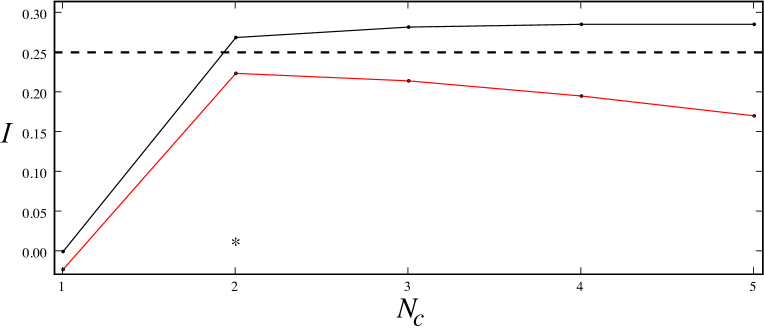
Figure 10: Information $I$ captured about the future versus the number $N_{c}$ of reconstructed states, with statistics estimated from length $T=100$ time series sample from the Golden Mean Process. Upper line: plotted on the vertical axis is $\widehat{I}[{\cal R};\stackrel{{\scriptstyle\rightarrow}}{{{X}}}\stackrel{{\scriptstyle{2}}}{{}}]_{\lambda\rightarrow 0}$ (not corrected); lower line: plotted on the vertical axis is the quantity $\widehat{I}[{\cal R};\stackrel{{\scriptstyle\rightarrow}}{{{X}}}\stackrel{{\scriptstyle{2}}}{{}}]_{\lambda\rightarrow 0}^{\rm corrected}$, which is the retained predictive information, but corrected for estimation errors due to finite sample size. The dashed line indicates the actual upper bound on the predictive information $I[\stackrel{{\scriptstyle\leftarrow}}{{{X}}}\stackrel{{\scriptstyle{K}}}{{}};{\cal R}]$, for comparison. This value is not known to the algorithm, it is computed from the true process statistics. Histories of length $K=3$ and futures of length $L=2$ were used. The asterisk denotes the optimal number ($N_{c}=2$) of effective states.

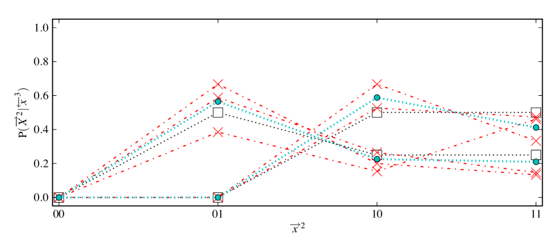
Figure 11: OCE’s best two-state approximated future conditional probabilities (circles) for the Golden Mean Process. Compared to true (unknown) future conditional probabilities (squares). The OCE inputs are the estimates of $\widehat{{\rm P}}(\stackrel{{\scriptstyle\rightarrow}}{{{X}}}\stackrel{{\scriptstyle{2}}}{{}}|\stackrel{{\scriptstyle\leftarrow}}{{{x}}}\stackrel{{\scriptstyle{3}}}{{}})$ (crosses).

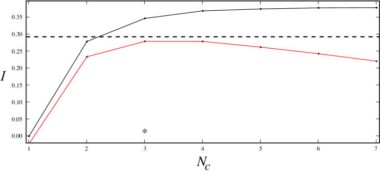
Figure 12: Information $I$ captured about the future versus the number $N_{c}$ of reconstructed states, with statistics estimated from length $T=100$ time series sample from the Even Process. Upper line: $\widehat{I}[{\cal R};\stackrel{{\scriptstyle\rightarrow}}{{{X}}}\stackrel{{\scriptstyle{2}}}{{}}]_{\lambda\rightarrow 0}$, not corrected; lower line: $\widehat{I}[{\cal R};\stackrel{{\scriptstyle\rightarrow}}{{{X}}}\stackrel{{\scriptstyle{2}}}{{}}]_{\lambda\rightarrow 0}^{\rm corrected}$, corrected for estimation error due to finite sample size. The dashed line indicates the actual upper bound on the predictive information, for comparison. This value is not known to the algorithm, it is computed from the true process statistics. Histories of length $K=3$ and futures of length $L=2$ were used. The asterisk denotes the optimal number ($N_{c}=3$) of effective states.

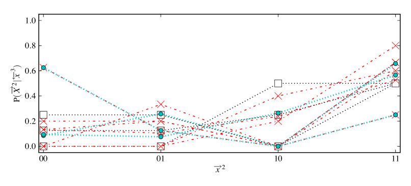
Figure 13: OCE’s best three-state approximated future conditional probabilities (circles) for the Even Process (d). Compared to true (unknown) future conditional probabilities (squares). The OCE inputs are the estimates of $\widehat{{\rm P}}(\stackrel{{\scriptstyle\rightarrow}}{{{X}}}\stackrel{{\scriptstyle{2}}}{{}}|\stackrel{{\scriptstyle\leftarrow}}{{{x}}}\stackrel{{\scriptstyle{3}}}{{}})$ (crosses).

We illustrate OCE on the Golden Mean and Even Processes studied in Sec. V. With the correct number of underlying states, they can be predicted at a substantial compression. Figures 10 and 12 show the mutual information $I[{\cal R};\stackrel{{\scriptstyle\rightarrow}}{{{X}}}\stackrel{{\scriptstyle{2}}}{{}}]$ versus the number $N_{c}$ of inferred states, with statistics estimated from time series of lengths $T=100$. The graphs compare the mutual information $\widehat{I}[{\cal R};\stackrel{{\scriptstyle\rightarrow}}{{{X}}}\stackrel{{\scriptstyle{2}}}{{}}]_{\lambda\rightarrow 0}$ evaluated using the estimate $\widehat{{\rm P}}(\stackrel{{\scriptstyle\rightarrow}}{{{X}}}\stackrel{{\scriptstyle{2}}}{{}};\stackrel{{\scriptstyle\leftarrow}}{{{X}}}\stackrel{{\scriptstyle{3}}}{{}})$ (upper curve) to the corrected information $\widehat{I}[{\cal R};\stackrel{{\scriptstyle\rightarrow}}{{{X}}}\stackrel{{\scriptstyle{2}}}{{}}]_{\lambda\rightarrow 0}^{\rm corrected}$ calculated by subtracting the approximated error Eq. (25) with $k^{L}=4$ and $M=96$ (lower curve).

We see that the corrected information curves peak at, and thereby, select models with two states for the Golden Mean Process and three states for the Even Process. This corresponds with the true number of causal states, as we know from above (Sec. V) for the two processes. The true statistical complexity for both processes is ${C_{\mu}}\approx 0.91830$, while those estimated via OCE are ${C_{\mu}}\approx 0.93773$ and ${C_{\mu}}\approx 1.30262$, respectively. (Recall that the overestimate for the latter was explained in Sec. V.3.)

Figures 11 and 13 show the OCE future conditional probabilities corresponding to the (optimal) two- and three-state approximations, respectively. The input to OCE are the future conditional probabilities given the histories $\widehat{{\rm P}}(\stackrel{{\scriptstyle\rightarrow}}{{{X}}}\stackrel{{\scriptstyle{2}}}{{}}|\stackrel{{\scriptstyle\leftarrow}}{{{x}}}\stackrel{{\scriptstyle{3}}}{{}})$ (crosses), which are estimated from the full historical information. Those future conditional probabilities are corrupted by sampling errors due to the finite data set size and differ from the true future conditional probabilities (squares).

Compare the OCE future conditional probabilities (circles) to the true future conditional probabilities (squares), calculated with the knowledge of the causal states. (The latter, of course, is not available to the OCE algorithm.) In the case of the GM Process, OCE approximates the correct future conditional probabilities. For the Even Process there is more spread in the estimated OCE future conditional probabilities. Nonetheless, OCE reduced the fluctuations in its inputs and corrected in the direction of the true underlying future conditional probabilities.

VII Conclusion

We analyzed an information-theoretic approach to causal modeling in two distinct cases: (i) optimal causal filtering (OCF), where we have access to the process statistics and desire to capture the process’s structure up to some level of approximation, and (ii) optimal causal estimation (OCE), in which, in addition, finite-data fluctuations need to be traded-off against approximation error and structure. The objective function used in both cases follows from very simple first principles of information processing and causal modeling: a good model should minimize prediction error at minimal model complexity. The resulting principle of using small, predictive models follows from minimal prior knowledge that, in particular, makes no structural assumptions about a process’s architecture: Find variables that do the best at causal shielding.

OCF stands in contrast with other approaches. Hidden Markov modeling, for example, assumes a set of states and an architecture (Rabiner and Juang, 1986). OCF finds these states from the given data. In minimum description length modeling, to mention another contrast, the model complexity of a stochastic source diverges (logarithmically) with the data set size (Rissanen, 1989), as happens even when modeling the ideal random process of a fair coin. OCF, however, finds the simplest (smallest) models.

Our main result is that OCF reconstructs the causal-state partition, a representation previously known from computational mechanics that captures a process’s causal architecture and that allows important system properties, such as entropy rate and stored information, to be calculated (Crutchfield and Shalizi, 1999). This result is important as it gives a structural meaning to the solutions of the optimization procedure specified by the causal inference objective function. We have shown that in the context of time series modeling, where there is a natural relevant variable (the future), the IB approach (Tishby et al., 1999) recovers the unique minimal sufficient statistic—the causal states—in the limit in which prediction is paramount to compression. Altogether, this allows us to go beyond plausibility arguments for the information-theoretic objective function that have been used. We showed that this way (OCI) of phrasing the causal inference problem in terms of causal shielding results in a representation that is a sufficient statistic and minimal and, moreover, reflects the structure of the process that generated the data. OCI does so in a way that is meaningful and well grounded in physics and nonlinear dynamics. The optimal solutions to balancing prediction and model complexity take on meaning—asymptotically, they are the causal states.

The results also contribute to computational mechanics: The continuous trade-off allows one to extend the deterministic history-to-state assignments that computational mechanics introduced to “soft” partitions of histories. The theory gives a principled way of constructing stochastic approximations of the ideal causal architecture. The resulting approximated models can be substantially smaller and so will be useful in a number of applications.

Finally, we showed how OCF can be adapted to correct for finite-data sampling fluctuations and so not over-fit. This reduces the tendency to see structure in noise. OCE finds the correct number of hidden causal states. This renders the method useful for application to real data.

References

- Berge et al. (1986) P. Berge, Y. Pomeau, and C. Vidal, Order within chaos (Wiley, New York, 1986).
- Guckenheimer and Holmes (1983) J. Guckenheimer and P. Holmes, Nonlinear Oscillations, Dynamical Systems, and Bifurcations of Vector Fields (Springer-Verlag, New York, 1983).
- Wiggins (1988) S. Wiggins, Global Bifurcations and Chaos: analytical methods (Springer-Verlag, New York, 1988).
- Devaney (1989) R. L. Devaney, An Introduction to Chaotic Dynamical Systems (Addison-Wesley, Redwood City, California, 1989).
- Lieberman and Lichtenberg (1993) A. J. Lieberman and M. A. Lichtenberg, Regular and Chaotic Dynamics (Springer-Verlag, New York, 1993), 2nd ed.
- Ott (1993) E. Ott, Chaos in Dynamical Systems (Cambridge University Press, New York, 1993).
- Strogatz (1994) S. H. Strogatz, Nonlinear Dynamics and Chaos: with applications to physics, biology, chemistry, and engineering (Addison-Wesley, Reading, Massachusetts, 1994).
- Packard et al. (1980) N. H. Packard, J. P. Crutchfield, J. D. Farmer, and R. S. Shaw, Phys. Rev. Let. 45, 712 (1980).
- Takens (1981) F. Takens, in Symposium on Dynamical Systems and Turbulence, edited by D. A. Rand and L. S. Young (Springer-Verlag, Berlin, 1981), vol. 898, p. 366.
- Fraser (1991) A. Fraser, in Information Dynamics, edited by H. Atmanspacher and H. Scheingraber (Plenum, New York, 1991), vol. Series B: Physics Vol. 256 of NATO ASI Series, p. 125.
- Crutchfield and McNamara (1987) J. P. Crutchfield and B. S. McNamara, Complex Systems 1, 417 (1987).
- Casdagli and Eubank (1992) M. Casdagli and S. Eubank, eds., Nonlinear Modeling, SFI Studies in the Sciences of Complexity (Addison-Wesley, Reading, Massachusetts, 1992).
- Sprott (2003) J. C. Sprott, Chaos and Time-Series Analysis (Oxford University Press, Oxford, UK, 2003), 2nd ed.
- Kantz and Schreiber (2006) H. Kantz and T. Schreiber, Nonlinear Time Series Analysis (Cambridge University Press, Cambridge, UK, 2006), 2nd ed.
- Crutchfield and Young (1989) J. P. Crutchfield and K. Young, Phys. Rev. Let. 63, 105 (1989).
- Tishby et al. (1999) N. Tishby, F. Pereira, and W. Bialek, in Proceedings of the 37th Annual Allerton Conference, edited by B. Hajek and R. S. Sreenivas (University of Illinois, 1999), pp. 368–377.
- Still and Bialek (2004) S. Still and W. Bialek, Neural Computation 16(12), 2483 (2004).
- Shalizi and Crutchfield (2002) C. R. Shalizi and J. P. Crutchfield, Advances in Complex Systems 5, 1 (2002).
- Shannon (1948) C. E. Shannon, Bell Sys. Tech. J. 27 (1948), reprinted in C. E. Shannon and W. Weaver The Mathematical Theory of Communication, University of Illinois Press, Urbana, 1949.
- Still and Crutchfield (2007) S. Still and J. P. Crutchfield (2007), arxiv.org: 0708.0654 [physics.gen-ph].
- Crutchfield (1994) J. P. Crutchfield, Physica D 75, 11 (1994).
- Crutchfield and Shalizi (1999) J. P. Crutchfield and C. R. Shalizi, Physical Review E 59, 275 (1999).
- Cover and Thomas (2006) T. M. Cover and J. A. Thomas, Elements of Information Theory (Wiley-Interscience, New York, 2006), 2nd ed.
- Crutchfield et al. (2009) J. P. Crutchfield, C. J. Ellison, and J. R. Mahoney, Phys. Rev. Lett. 103, 094101 (2009).
- Crutchfield and Feldman (2003) J. P. Crutchfield and D. P. Feldman, CHAOS 13, 25 (2003).
- Bialek et al. (2006) W. Bialek, R. R. de Ruyter van Steveninck, and N. Tishby, in Proceedings of the International Symposium on Information Theory (2006), pp. 659–663.
- del Junco and Rahe (1979) A. del Junco and M. Rahe, Proc. AMS 75, 259 (1979).
- Crutchfield and Packard (1983) J. P. Crutchfield and N. H. Packard, Physica 7D, 201 (1983).
- Shaw (1984) R. Shaw, The Dripping Faucet as a Model Chaotic System (Aerial Press, Santa Cruz, California, 1984).
- Grassberger (1986) P. Grassberger, Intl. J. Theo. Phys. 25, 907 (1986).
- Li (1991) W. Li, Complex Systems 5, 381 (1991).
- Bialek and Tishby (1999) W. Bialek and N. Tishby, Predictive information (1999), URL arXiv:cond-mat/9902341v1.
- Crutchfield et al. (2010) J. P. Crutchfield, C. J. Ellison, J. R. Mahoney, and R. G. James, CHAOS p. in press (2010).
- Arimoto (1972) S. Arimoto, IEEE Transactions on Information Theory IT-18 pp. 14–20 (1972).
- Blahut (1972) R. E. Blahut, IEEE Transactions on Information Theory IT-18 pp. 460–473 (1972).
- Rose et al. (1990) K. Rose, E. Gurewitz, and G. C. Fox, Phys. Rev. Lett. 65, 945 (1990).
- Rose (1998) K. Rose, Proc. of the IEEE 86, 2210 (1998).
- Ellison et al. (2009) C. J. Ellison, J. R. Mahoney, and J. P. Crutchfield, J. Stat. Phys. 136, 1005 (2009).
- Strelioff et al. (2007) C. C. Strelioff, J. P. Crutchfield, and A. Hübler, Phys. Rev. E 76, 011106 (2007).
- Rabiner and Juang (1986) L. R. Rabiner and B. H. Juang, IEEE ASSP Magazine January (1986).
- Rissanen (1989) J. Rissanen, Stochastic Complexity in Statistical Inquiry (World Scientific, Singapore, 1989).
- Still (2009) S. Still, Euro. Phys. Lett. 85, 28005 (2009).
- Ay and Crutchfield (2005) N. Ay and J. P. Crutchfield, J. Stat. Phys. 210, 659 (2005).