Resonance phenomena in discrete systems with bichromatic input signal

Abstract

We undertake a detailed numerical study of the twin phenomenon of stochastic and vibrational resonance in a discrete model system in the presence of bichromatic input signal. A two parameter cubic map is used as the model that combines the features of both bistable and threshold settings. Our analysis brings out several interesting results, such as, the existence of a cross over behavior from vibrational to stochasic resonance and the possibility of using stochastic resonance as a filter for the selective detection/transmission of the component frequencies in a composite signal. The study also reveals a fundamental difference between the bistable and threshold mechanisms with respect to amplification of a multi signal input.

1 Introduction

During the last two decades, investigation of signal processing in nonlinear systems in the presence of noise has revealed several interesting phenomena, the most important being stochastic resonance(SR)[1]. It can roughly be considered as the optimisation of certain system performance by noise. The interest in the study of nonlinear noisy systems has increased due to the applications in the modelling of a great variety of phenomena of relevance in physics,chemistry and lifesciences[1-3].

In SR, the response of a nonlinear system to a weak input signal is significantly increased with appropriate tuning of the noise intensity[1]. When a subthreshold signal $I(t)$ is input to a nonlinear system $g$ together with a noise $\zeta(t)$, if the filtered output $O(t)\equiv g(I(t)+\zeta(t))$ shows enhanced response that contains the information content of $I(t)$, then SR is said to be realised in the system. The mechanism first used by Benzi, Nicolis etc [4,5] to explain natural phenomena is now being used for a large variety of interesting applications like modelling biological and ecological systems [6], lossless communication purposes etc [7]. Apart from these, it has opened up a vista of many related resonance phenomena [8] which are equally challenging from the point of view of intense research. The most important among these, which closely resembles SR, is the vibrational resonance (VR) [9], where a high frequency forcing plays the role of noise and amplify the response to a low frequency signal in bistable systems. In VR, analogous to SR, the system response shows a bell shaped resonant form as a function of the amplitude of the high frequency signal. In this work, we try to capture numerically some interesting and novel aspects of SR and VR, using a simple discrete model, namely, a two parameter bimodal cubic map.

In the early stages of the development of SR, most of the studies were done using a dynamical setup with bistability, modelled by a double well potential. Here SR is realised due to the shuttling between the two stable states at the frequency of the subthreshold signal with the help of noise. Thus if the potential is

$$V(X)=-aX^{2}/2+bX^{4}/4$$ (1)

in the presence of a signal and noise, the dynamics can be modelled by an overdamped oscillator

$$\dot{X}=aX-bX^{3}+ZSin\omega t+E\zeta(t)$$ (2)

If $C_{th}$ is the threshold at which deterministic switching (with noise amplitude $E=0$) is possible, then well to well switching due to SR occurs when

$$-C_{th}>(ZSin\omega t+E\zeta(t))>C_{th}$$ (3)

that is, twice in one period of the signal $T=2\pi/\omega$.

The characterisation of SR in this case is most commonly done by computing the signal to noise ratio (SNR) from the power spectrum of the output as

$$SNR=10log_{10}(S/N)dB$$ (4)

where $N$ is the average background noise around the signal $S$. If SR occurs in the system, then the SNR goes through a maximum giving a bell shaped curve as $E$ is tuned.

SR has also been observed in systems with a single stable state with an escape scenerio. These threshold systems, in the simplest case, can be modelled by a piecewise linear system or step function

$$g(u)=-1\hskip 12.0ptu<C_{th}$$

$$\hskip 22.0pt=+1\hskip 12.0ptu>C_{th}$$

The escape with the help of noise is followed by resetting to the monostable state. In this case, a quantitative characterisation is possible directly from the output, but only in terms of probabilities. If $t_{n}$ are the escape times, the inter spike interval (ISI) is defined as $T_{n}=t_{n+1}-t_{n}$ and $m(T_{n})$ is the number of times the same $T_{n}$ occurs. For SR to be realised in the system, the probability $p_{n}=m(T_{n})/N$ ($N$ is the total number of escapes) has to be maximum corresponding to the signal period $T$ at an optimum noise amplitude.

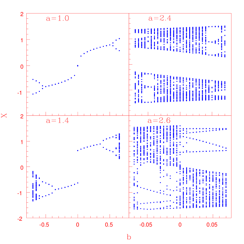
Figure 1: The bifurcation structure of the cubic map given in eq.(5) corresponding to four values of the parameter $a$, to show the bistability in periodic and chaotic attractors with the basin boundary at $X=0$. It is clear that the bistability just begins at $a=1.0$ and ends at $a=2.6$. Note that the range of $b$ values for bistability is different for periodic and chaotic attractors.

In the case of VR, the high frequency forcing takes the role of noise to boost the subthreshold signal. The system is then under the action of a two frequency signal, one of low frequency and the other of high frequency, with or without the presence of noise. Most of the studies in VR also have been done using the standard model of overdamped bistable oscillators [10]. But recently, VR has been shown to occur in a spatially extended system of coupled noisy oscillators [11] and two coupled anharmonic oscillators [12] in the bistable setup. In the threshold setup, VR has been shown to occur only in one system, namely, in the numerical simulation of the FitzHugh-Nagumo (FHN) model in the excitable regime along with the experimental confirmation using an electronic circuit [13]. Here we show for the first time the occurance of VR in a discrete system, both in bistable and threshold setups.

There are situations where SR and VR are to be optimised by adapting to or designing the dynamics of the system. This is especially relevant in natural systems where the noise is mostly from the environmental background and therefore not viable to fine tuning. Similarly, depending on the context or application, the nature of the signal can also be different, such as, periodic, aperiodic, digital, composite etc. The classical SR deals with the detection of a single subthreshold signal immersed in noise. However, in many practical situations, a composite signal consisting of two harmonic components in the presence of background noise is encountered, as for example, in biological systems for the study of planktons and human visual cortex [14], in laser physics [15] and in accoustics [16]. Studies involving such bichromatic signals are also relevant in communication, since one can address the question of the carrier signal itself amplifying the modulating signal. Moreover, two frequency signals are commonly used in multichannel optical communication systems based on wave length division multiplexing (WDM) [17]. But only very few studies of SR have been carried out using the bichromatic signals to date [18-21], each of them pertaining to some specific dynamical setups and with continuous systems. This is one of the motivations for us to undertake a detailed numerical analysis of SR and VR with such signals using a discrete model. It is a discretised version of the overdamped bistable oscillator, but with the added feature of an inherent escape mode also. Hence it can function in both setups, bistable and threshold, as a stochastic resonator.

There are many situations, especially in the biological context, such as, host-parasite model, virus-immune model etc., where discrete systems model the time developments directly. They can behave differently, especially in the presence of high frequency modulation and background noise. The benefit of high frequency forcing has been studied in the response of several biological phenomena[22]. High frequency stimulation treatments in Parkinson’s disease and other disorders in neuronal activity have also been reported[23]. Moreover, it is also known that optimum high frequency modulation improves processing of low frequency signal even in systems without bistability where noise can induce the required structure[11]. Thus a study of resonance phenomena in discrete systems can lead to qualitatively different results having potential practical applications. We do observe some novel features which have not been reported so far for continuous systems.

Our paper is organised as follows: In §2, the model system used for the analysis is introduced. In §3, we study SR in the model numerically with bichromatic signal treating it as a bistable system. Numerical and analytical results of VR in the bistable setup are presented in §4. §5 discusses SR and VR with the cubic map as a threshold system. Results and discussions are given given in §6.

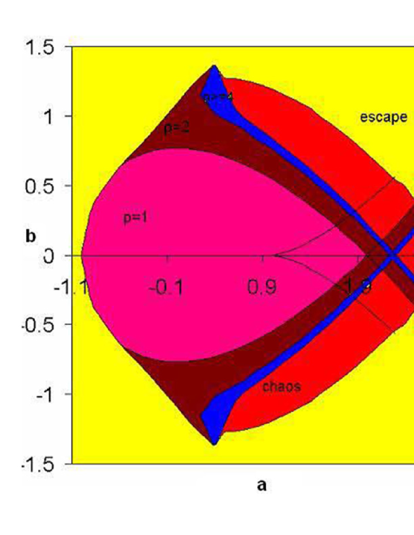
Figure 2: Parameter space plot in $(a,b)$ plane for the cubic map given by eq.(5). Regions of periodic attractors with period 1(p=1), period 2(p=2) etc. and that of chaotic attractors and escape are shown in different colours. Region within the quadrilaterals $(a>1.0)$ corresponding to $p=1,p=2$ and chaos represent the respective bistable regions.

2 The model system

The model used for our analysis is a two parameter cubic map given by

$$X_{n+1}=f(X_{n})=b+aX_{n}-X_{n}^{3}$$ (5)

It is a discrete version of the Duffing’s double well potential and is the simplest possible nonlinear discrete system that combines the desirable features of bistable and threshold setups. Hence it is extremely useful in the study of resonance phenomena caused by noise or high frequency signal. Similar systems in the continuous cases include the FHN model[23] for neuronal firing with two widely different time scales.

The system has been studied in great detail both analytically and numerically and has been shown to possess a rich variety of dynamical properties including bistability [24]. In particular, if $a_{1}$ is the value of the parameter at which $f^{\prime}(X_{i},a_{1},b)=1$, then for $a>a_{1}$, there is a window in $b$, where bistability is observed. The bistable attractors are clearly separated with $X>0$ being the basin of one and $X<0$ that of the other. It is found that for $a$ in the range $1.0<a<2.6$, the system has periodic states and chaotic states. As $a$ increases from $1.0$, the periodicity of the bistable attractors keep on doubling while the width of the window around $b$ decreases correspondingly. For $a=2.4$, two chaotic attractors co-exist in a very narrow window around $b$. For $a<1.0$, the system has a monostable period 1 state and for $a>2.6$, there is merging of the chaotic states followed by escape. All these can be clearly seen from Fig.1 where bifurcation structure of the cubic map corresponding to four $a$ values are shown. A detailed stability analysis fixes the different asymptotic behavior in its parameter plane $(a,b)$ as shown in Fig.2. Regions of periodicities $(p=1,p=2)$ etc., chaos and escape in the parameter plane can be clearly seen. The quadrilateral regions in the area marked $p=1,p=2$ and chaos represent bistability in the respective attractors.

The system when driven by a gaussian noise and a periodic signal becomes

$$X_{n+1}=b+aX_{n}-X_{n}^{3}+E\zeta(n)+ZF(n)$$ (6)

where we choose $\zeta(n)$ to be a gaussian noise time series with zero mean and $F(n)$ is the periodic signal sampled in unit time step. The amplitude of the noise and the signal can be varied by tuning E and Z respectively. It can be shown that in the regime of chaotic bistable attractors $(a=2.4,b=0.01)$, a subthreshold input signal can be detected using the inherent chaos in the system without any external noise(E=0). Taking the signal $F(n)=ZSin(2\pi\nu n)$, with $Z=0.16$, the system shows SR type behavior for an optimum range of frequencies as shown in Fig.3, where the output SNR is plotted as a function of the frequency $\nu$. It implies that a subthreshold signal can be detected by passing through a bistable system making use of the inherent chaos in it without the help of any external noise. This phenomenon is known as deterministic resonance. In the regime of periodic bistable attractors $(a=1.4,b=0.01)$ with a single subthreshold signal, the system shows conventional SR as well as chaotic resonance (CR), and using this model, we have recently reported some new results including enhancement of SNR via coupling [25].

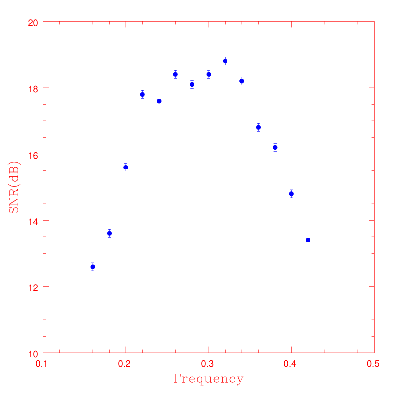
Figure 3: Variation of SNR with frequency for the bistable cubic map in the chaotic regime $(a=2.4)$ with the noise amplitude $E=0$. Note that a subthreshold signal $(Z=0.16)$ can be detected for an intermediate range of frequencies, without any external noise.

3 SR with bichromatic input signal

In this section, we undertake a numerical study of SR using the cubic map in the bistable regime. The input signal $F(n)$ is taken as a superposition of at least two fundamental frequencies, $\nu_{1}$ and $\nu_{2}$. Before going into the numerical results, we briefly mention some already known results for multisignal inputs in the case of over damped bistable potential.

The most popular theory for the analytical description of SR is the linear response theory(LRT)[26-29]. According to this theory, the response of a nonlinear stochastic system $X(t)$ to a weak external force $F(t)$ in the asymptotic limit of large times is determined by the integral relation [26]

$$X(t)=<X_{0}>+\int_{-\infty}^{\infty}R(t-\tau)F(\tau)d\tau$$ (7)

where $<X_{0}>$ is the mean value of the state variable for $F(t)=0$. Without lack of generality, one can set $<X_{0}>=0$. The function $R(t)$ in (7) is called the response function. For a harmonic signal, the system response can be expressed through the function $R(\omega)$ which is the Fourier transform of the response function:

$$X(t)=Z|R(\omega)|Sin(2\pi\nu t+\psi)$$ (8)

where $\psi$ is a phase shift.

The LRT can be naturally extended to the case of multifrequency signals. Let the signal $F(t)$ be a composite signal of the form:

$$F(t)=Z\sum_{k=1}^{n}Sin(2\pi\nu_{k}t)$$ (9)

where $\nu_{k}$ are the frequencies of the discrete spectral components with the same amplitude $Z$. Then according to LRT, the system response can be shown to be [29]

$$X(t)=Z\sum_{k=1}^{n}|R(\omega_{k})|Sin(2\pi\nu_{k}t+\psi_{k})$$ (10)

which contains the same spectral components at the input. We now show numerically that the same is true for a discrete system as well, in the bistable setup.

For the remaining part of the paper, we fix $a=1.4$ and $b=0.01$ in the region of bistable periodic attractors and $\zeta(n)$ is a gaussian time series whose amplitude can be tuned by changing the value of $E$. The system is driven by a composite signal consisting of a combination of two frequencies $\nu_{1}$ $\nu_{2}$, given by

$$ZF(n)=Z(Sin2\pi\nu_{1}n+Sin2\pi\nu_{2}n)$$ (11)

The value of $Z$ is fixed at $0.16$ so that the signal is well below threshold. It should be noted that because of the iteration with unit time step $(ie,n=1,2,3,...)$, the available range of frequencies is limited to $\nu_{k}\equiv(0,0.5)$. We use different combination of frequencies $(\nu_{1},\nu_{2})$ for numerical simulation in the presence of noise by tuning the value of $E$. For convenience, $\nu_{1}$ is fixed at $0.125$ and $\nu_{2}$ is varied from $0.02$ to $0.5$ in steps of $0.01$. For each selected combination, the output power spectrum is calculated using the FFT algorithm for different values of $E$. A typical power spectrum for $(\nu_{1},\nu_{2})=(0.125,0.05)$ is shown in Fig.4(a). The procedure is repeated with $F(n)$ consisting of a combination of 3 frequencies and a power spectrum for $(\nu_{1},\nu_{2},\nu_{3})=(0.125,0.075,0.2)$ is shown in Fig.4(b). To compute the power spectrum, only the inter-well transitions are taken into account and all the intra-well fluctuations are suppressed with a two state filtering. It is clear that, only the fundamental frequencies present in the input are enhanced.

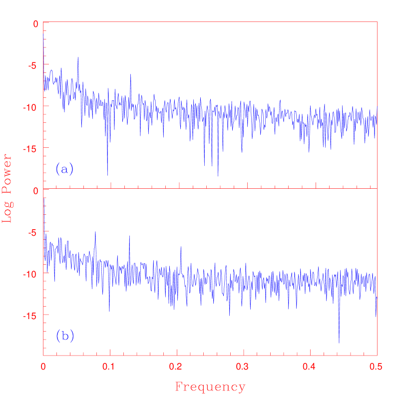
Figure 4: Power spectrum for the bistable system (6) with a composite signal consisting of $(a)$ 2 frequencies $(\nu_{1},\nu_{2})=(0.125,0.05)$ and $(b)$ 3 frequencies $(\nu_{1},\nu_{2},\nu_{3})=(0.125,0.075,0.2)$, with $Z=0.16$ and $E=0.4$ in both cases. The system parameters are $a=1.4$ and $b=0.01$.

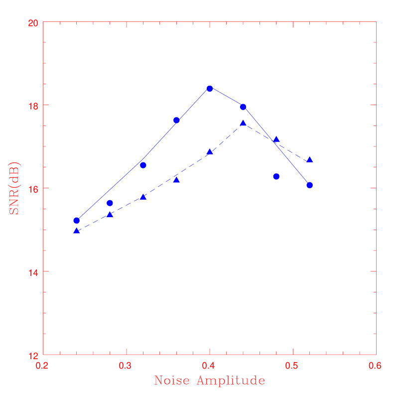
Figure 5: Variation of SNR with noise amplitude for the 2 frequencies shown in $Fig.4(a)$, with the filled circle connected by solid line representing the higher frequency $\nu_{1}$.

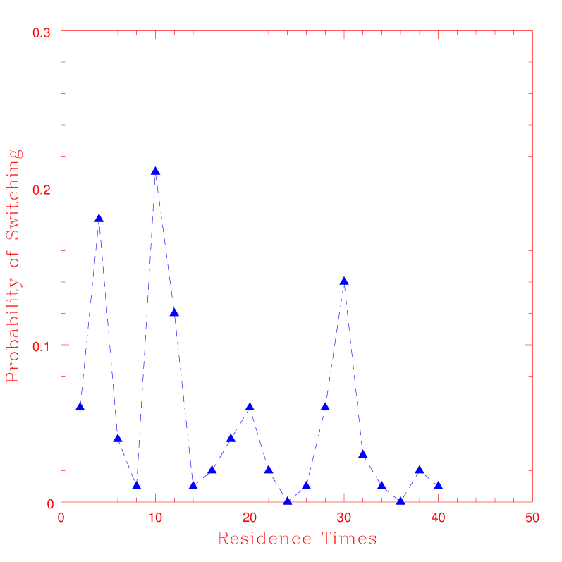
Figure 6: The RTDF for the system (6), with a composite signal consisting of 2 frequencies $\nu_{1}=0.125$ and $\nu_{2}=0.05$ and amplitude $Z=0.16$. The noise amplitude is put at the optimum value $0.4$. Note that the peaks are synchronised with half the periods corresponding to the input frequencies.

We now concentrate on a combination of 2 frequencies and compute the two important quantifiers of SR, namely, the SNR and the Residence Time Distribution Function(RTDF). For the frequencies in Fig.4(a), the SNR is computed from the power spectrum using equation (4) for a range of values of $E$ and the results are shown in Fig.5. The RTDF measures the probability distribution of the average times the system resides in one basin, as a function of different periods. If T is the period of the applied signal, the distribution will have peaks corresponding to times $(2n+1)T/2$, n=0,1,2…For the system (6) with $(\nu_{1},\nu_{2})=(0.125,0.05)$, the results are shown in Fig.6. Note that there are only peaks corresponding to the half integer periods of the two applied frequencies.

The above computations are repeated taking various combinations of frequencies $(\nu_{1},\nu_{2})$, both commensurate and non-commensurate. For a fixed combination of $(\nu_{1},\nu_{2})$, the calculations are also done by changing the signal amplitude $Z$ of one and both signals. Always the results remain qualitatively the same and only the fundamental frequencies present in the input are amplified at the output. If $Z$ becomes very small $(<0.1)$ compared to the noise level, then the phenomenon of SR disappears altogether and the signal remains undetected in the background noise.

In all the above computations, we used additive noise, where the noise has been added to the system externally. But in many natural systems, noise enters through an interaction of the system with the surroundings, that is, through a parameter modulation, rather than a simple addition. Such a multiplicative noise occurs in a variety of physical phenomena [30] and can, in principle, show qualitatively different behavior in the presence of a periodic field [31]. To study its effect on the bistable system, equation (6) is modified as

$$X_{n+1}=b+a(1+E\zeta(n))X_{n}-X_{n}^{3}+ZF(n)$$ (12)

The noise is added through the parameter $a$ which determines the nature of the bistable attractors. With $a=1.4$ and $b=0.01$, the system is now driven by a signal of single frequency $\nu_{1}=0.125$ and a multisignal with 2 frequencies $(\nu_{1},\nu_{2})$, with $Z=0.16$. The power spectrum for single frequency and multiple frequencies are shown in Fig.7(a) and (b) respectively. The corresponding SNR variation with noise $E$ are shown in Fig.8(a) and (b). Note that the results are qualitatively identical to that of additive noise, but the optimum SNR and the corresponding noise amplitude are comparitively much higher in this case. Thus our numerical results indicate that a bistable system responds only to the fundamental frequencies in a composite signal and not to any mixed modes.

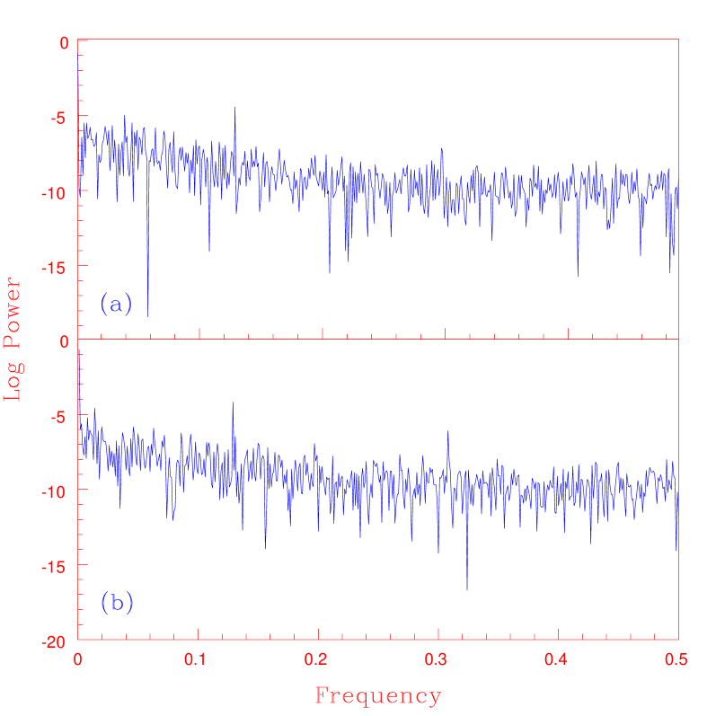
Figure 7: The power spectrum for the bistable system (12), with the signal $F(n)$ consisting of $(a)$ one frequency $\nu_{1}=0.125$ and $(b)$ 2 frequencies $\nu_{1}=0.125$ and $\nu_{2}=0.3$. The parameter values used are $Z=0.16,E=1.0,a=1.4$ and $b=0.01$.

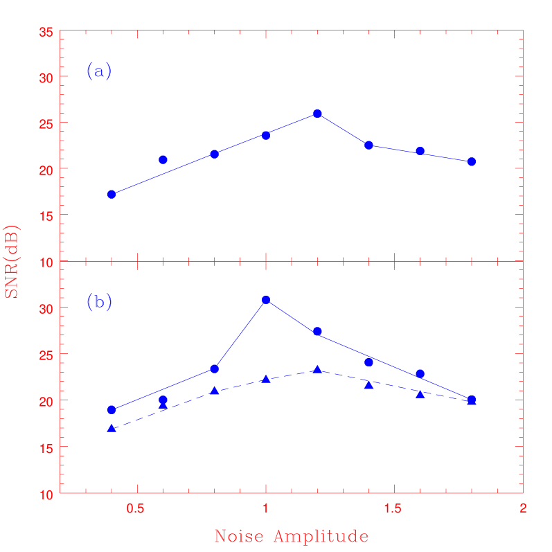
Figure 8: Variation of SNR with noise for the system(12), for $(a)$ single frequency $\nu_{1}=0.125$ and $(b)$ 2 frequencies $\nu_{1}=0.125$ (filled circles) and $\nu_{2}=0.3$. Note that the optimum SNR of $\nu_{1}$ increases by about 5 dB when a second signal $\nu_{2}$ is added.

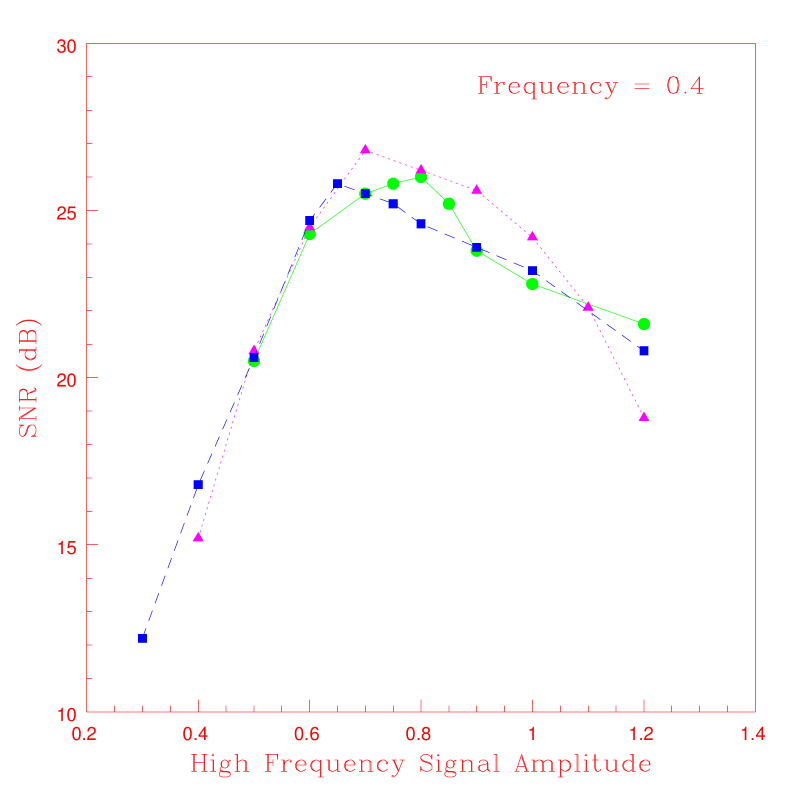
Figure 9: Variation of SNR corresponding to the frequency $\nu_{1}=0.125$ as a function of the amplitude $Z(2)$ of the high frequency signal with $\nu_{2}=0.4$, showing VR in the bistable cubic map with a bichromatic input signal given by eq.(13). The three curves correspond to different values of noise amplitude, namely, $E=0.06$ (circle connected by solid line), $E=0.12$ (triangle connected by dotted line) and $E=0.16$ (squares conneted by dashed line). The optimum values of $Z(2)$ shifts towards the left as $E$ increases.

4 VR: Numerical and analytical results

In order to study VR in the system, the input periodic driving is modified as

$$ZF(n)=Z(1)Sin(2\pi\nu_{1}n)+Z(2)Sin(2\pi\nu_{2}n)$$ (13)

where $\nu_{1}$ is the low frequency signal which is fixed at $0.125$ with its amplitude $Z(1)$ at the subthreshold level $0.16$. It is added with a signal of high frequency $\nu_{2}(>\nu_{1})$ whose amplitude $Z(2)$ is tuned to get VR. We have used a number of values for $\nu_{2}$ over a wide range from $0.15$ to $0.5$ to study VR in the system. A small amount of noise is also added as in eq.(6) which represents tiny random fluctuations present in all practical systems.

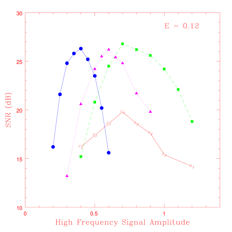
Figure 10: Variation of SNR for $\nu_{1}$ as a function of $Z(2)$ corresponding to four values of $\nu_{2}$ which are $0.18$ (filled circle connected by solid line), $0.32$ (triangles connected by dotted line), $0.40$ (squares connected by dashed line) and $0.46$ (open circles connected by solid line). As $\nu_{2}>>\nu_{1}$, it becomes less effective in producing VR as indicated by the reduction in the optimum value of SNR.

By taking $\nu_{2}=0.4$ and $E=0.12$, the system is iterated by tuning the high frequency signal amplitude. The variation of SNR for the signal computed from the output time series as a function of $Z(2)$, clearly indicates VR in the system. The procedure is repeated by changing $E$ to study the influence of noise level on VR. The results are shown in Fig.9 for 3 values of $E$. It is found that as $E$ decreases, the optimum SNR shifts towards the higher value of $Z(2)$. This result has been reported earlier in the case of continuous systems also[10,12].

The computations are repeated by taking different values of $\nu_{2}$ in the range $0.15$ to $0.5$ by fixing $E=0.12$. The SNR as a function of $Z(2)$ for four values of $\nu_{2}$ are shown in Fig.10. Two results are evident from the figure. The optimum SNR is independant of the high frequency when $(\nu_{2}-\nu_{1})$ is small. But for $\nu_{2}>>\nu_{1}$, the optimum SNR decreases appreciably. This implies that the effectiveness of the high frequency in producing VR is reduced as it becomes too large compared to the low frequency signal. It can also be seen that the optimum value of $Z(2)$ depends on $\nu_{2}$. Infact, it increases with $\nu_{2}$. Thus, a higher value of $\nu_{2}$ requires a larger amplitude and becomes less effective as $\nu_{2}>>\nu_{1}$.

One reason for this is that, due to the unit time sampling of the signals, the fluctuation in the signal values will be more as the frequency increases. Hence the average will be closer to zero, higher the frequency, which makes it necessary to have larger amplitude. But once the optimum amplitude becomes too large, escape becomes possible in all time scales making it less effective. It can also be shown that the high frequency forcing can change the effective value of the parameter $a$ so that the map can come out of the bistable window. This is discussed in more detail below.

The dependance of optimum $Z(2)$ on $\nu_{2}$ also implies that the system shows the so called bona fide resonance[32,33]. This is shown in Fig.11, where the SNR is plotted as a function of the high frequency for two values $(0.5\&0.7)$ of $Z(2)$, with $E$ fixed at $0.12$.

We now briefly discuss some analytical results for VR in the cubic map and show that the high frequency forcing can change the effective value of the parameter $a$. Here we consider the case $\nu_{2}>>\nu_{1}$, in the noise free limit, $E=0$. In parallel with the theory developed to explain VR in continuous systems[34], we analyse the effect of the widely differing frequencies for the system under study:

$$X_{n+1}=b+aX_{n}-X_{n}^{3}+ASin\omega_{1}n+BSin\omega_{2}n$$ (14)

where $\omega_{1,2}=2\pi\nu_{1,2}$. Taking $A=0$, we look for a solution[34]

$$X_{n}=Y_{n}-{{BSin\omega_{2}n}\over{\omega_{2}^{2}}}$$ (15)

While the first term $Y_{n}$ varies significantly only over time of the order $n$, the second term varies rapidly within an iteration and hence can be averaged. Putting (15) in (14) and averaging, we get:

$$Y_{n+1}=b+aY_{n}-Y_{n}^{3}-{{3Y_{n}B^{2}}\over{2\omega_{2}^{2}}}$$ (16)

That is,

$$Y_{n+1}=b+a^{*}Y_{n}-Y_{n}^{3}$$ (17)

where

$$a^{*}=a-{{3B^{2}}\over{2\omega_{2}^{2}}}$$ (18)

Thus the effect of the high frequency forcing is to reset the parameter $a$ as $a^{*}$. Hence only for the choice of $B$ and $\omega_{2}$ that retains $a^{*}$ in the bistable window $(1.0<a^{*}<2.6)$, do we expect shuttling behavior at the low frequency signal for $A\neq 0$. Now the lower limit for $a$ becomes

$$a\geq 1.0+{{3B^{2}}\over{2\omega_{2}^{2}}}$$ (19)

which gives

$$({{B}\over{\omega_{2}^{2}}})^{2}\leq{{{2}\over{3}}(a-1.0)}$$ (20)

Thus, for a given choice of $a$, there is an upper limit for $({{B}\over{\omega_{2}}})$ for retaining the bistability in the system. The actual values may get modified in the presence of noise. Also, this mechanism provides two parameters $B$ and $\omega_{2}$ that can be tuned in a mutually compramisable manner to obtain VR or even SR with added noise. Moreover, even when $a>2.6$, $a^{*}$ can be $<2.6$ and hence this increases the virtual window of bistability in the system providing greater range for applicability.

5 SR and VR in the threshold setup

As said earlier, the domains of the bistable attractors in the cubic map are clearly separated with the boundary $X=0$. Hence the cubic map can also be considered as a nondynamical threshold system with a single stable state having a potential barrier. Here the system generates an output spike only when the combined effort of the signal and the noise pushes it across the potential barrier $(atX=0)$ in one direction:

$$[E\zeta(n)+ZF(n)]>C_{th}$$ (21)

It is then externally reinjected back into the basin. The output thus consists of a series of spikes similar to a random telegraph process. The study of SR and VR in such systems assumes importance in the context of biological applications and in particular the integrate and fire models of neurons where SR and VR have been firmly established[3,35].

The computations are done using equation (6), initially with a single frequency signal, $F(n)=Sin(2\pi\nu_{1}n)$. We start from an initial condition in the negative basin and when the output crosses the threshold, $X=0$, it is reinjected back into the basin by resetting the initial conditions. This is repeated for a sufficiently large number of escapes and the ISIs are calculated. The ISIs are then normalised in terms of the periods $T_{n}$ and the probability of escape corresponding to each $T_{n}$ is calculated as the ratio of the number of times $T_{n}$ occurs to the total number of escapes. The whole procedure is repeated tuning the noise amplitude $E$. It is found that the ISI is synchronised with the period of the forcing signal for an optimum noise amplitude (Fig.12), indicating SR for the frequency $\nu_{1}$.

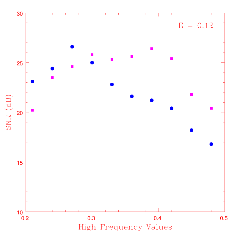
Figure 11: Evidence for bona-fide resonance in the cubic map. Variation of SNR corresponding to $\nu_{1}=0.125$ as function of the high frequency $\nu_{2}$ for two values of its amplitude, namely, $Z(2)=0.5$ (circles) and $Z(2)=0.7$ (squares). The amplitude of $\nu_{1}$ is fixed at $0.16$ and $E=0.12$.

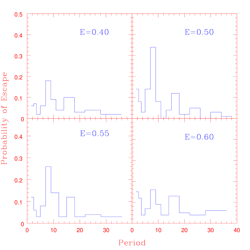
Figure 12: The probability of escape for the system (6) as a function of different periods, when it is used as a threshold system with the signal $F(n)$ having a single frequency $\nu_{1}=0.125$ and a subthreshold amplitude $Z=0.16$. The escape probability is plotted corresponding to four different noise amplitudes $E$. Note that the probability corresponding to the signal period $(T=8)$ passes through an optimum value for $E=0.5$.

The calculations are now repeated by adding a second signal of frequency $\nu_{2}$ and amplitude same as that of $\nu_{1}$. Again different values of $\nu_{2}$ in the range $0.02$ to $0.5$ are used for the calculation. It is then found that apart from the input frequencies $\nu_{1}$ and $\nu_{2}$, a third frequency, which is a mixed mode is also enhanced at the output, at a lesser value of the noise amplitude. To make it clear, the amplitude $Z$ of both $\nu_{1}$ and $\nu_{2}$ are reduced from $0.16$ to $0.08$, so that they become too weak to get amplified. The results of computations are shown in Fig.13 and Fig.14, for a combination of input signals $(\nu_{1},\nu_{2})=(0.125,0.033)$. Fig.13 represents the probability of escape corresponding to different periods, for the optimum value of noise. It is clear that only a very narrow band of frequencies $d\nu$ around a third frequency $\approx 0.045$ (corresponding to the period $T\approx 22s$), are amplified at the output. Note that this frequency is absent in the input and corresponds to $(\nu_{1}-\nu_{2})/2$. This is in sharp contrast to the earlier case of a bistable system. The variation of escape probability corresponding to this frequency as a function of noise amplitude is shown in Fig.14.

This result can be understood as follows: When two signals of frequencies $\nu_{1}$ and $\nu_{2}$ and equal amplitude $Z$ are superposed, the resulting signal consists of peaks of amplitude $2Z$ repeating with a frequency $(\nu_{1}-\nu_{2})/2$ in accordance with the linear superposition principle:

$$Sin(2\pi\nu_{1}t)+Sin(2\pi\nu_{2}t)=2Sin(2\pi\nu_{+}t)Cos(2\pi\nu_{-}t)$$ (22)

where $\nu_{+}=(\nu_{1}+\nu_{2})/2$ and $\nu_{-}=(\nu_{1}-\nu_{2})/2$. For a threshold system, the probability of escape depends only on the amplitude of the signal which is maximum corresponding to the frequency $\nu_{-}$. But in the case of a bistable system, the signal is enhanced only if there is a regular shuttling between the wells at the corresponding frequency. This is rather difficult for the frequency $\nu_{-}$ because, its amplitude is modulated by a higher frequency $\nu_{+}$. This result has been checked by using different combinations of frequencies $(\nu_{1},\nu_{2})$ and also with different amplitudes. It should be mentioned here that this result reveals a fundamental difference between the two mechanisms of SR and is independant of the model considered here. We have obtained identical results with a fundamentally different model showing SR, namely, a model for Josephson junction and has been discussed elsewhere[21].

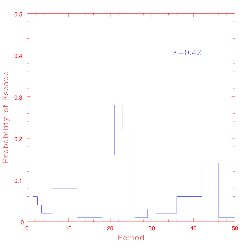
Figure 13: The escape probability corresponding to the optimum noise amplitude with the signal $F(n)$ comprising of 2 frequencies $\nu_{1}=0.125$ and $\nu_{2}=0.033$. The amplitudes of individual signals are put much below the threshold value required for SR. Note that only the difference frequency $(\nu_{1}-\nu_{2})/2$ is amplified.

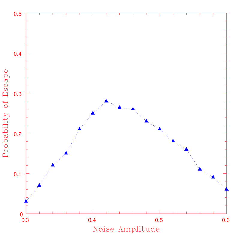
Figure 14: Variation of the probability of escape corresponding to the frequency shown in $Fig.13$, as a function of noise amplitude.

To study VR in the threshold set up, we once again consider the input signal as in eq.(13) with the low frequency $\nu_{1}$ fixed at $0.125$ and $Z(1)=0.16$. With $E=0.12$ and $\nu_{2}=0.32$, the computations are performed as before by tuning the high frequency amplitude $Z(2)$. The results are shown in Fig.15, which clearly indicates VR in the threshold set up. The computations are repeated for different values of $\nu_{2}$ and here also it is found that the optimum escape probability becomes less for $\nu_{2}>0.45$ as in the bistable case.

It is interesting to note that when the high frequency forcing and noise are present simultaneously, only one of them dominates to enhance the signal. In the regime of VR, the noise level has to be small enough and vice versa for SR. When both are high, the transitions become random and the signal is lost. We find that the two regimes of (VR and SR) can be distinguished in terms of an initial time delay for the system to respond to the high frequency or noise, called the response time. The response time $(\tau)$ decreases sharply in the regime of SR (ie, when signal is boosted with the help of noise), thus indicating a cross over behavior between the two regimes. This is shown in Fig.16, where $\tau$ is plotted as a function of $E$ for the threshold setup. The computations are done in such a way that as $E$ is increased, $Z(2)$ is decreased correspondingly to get optimum response.

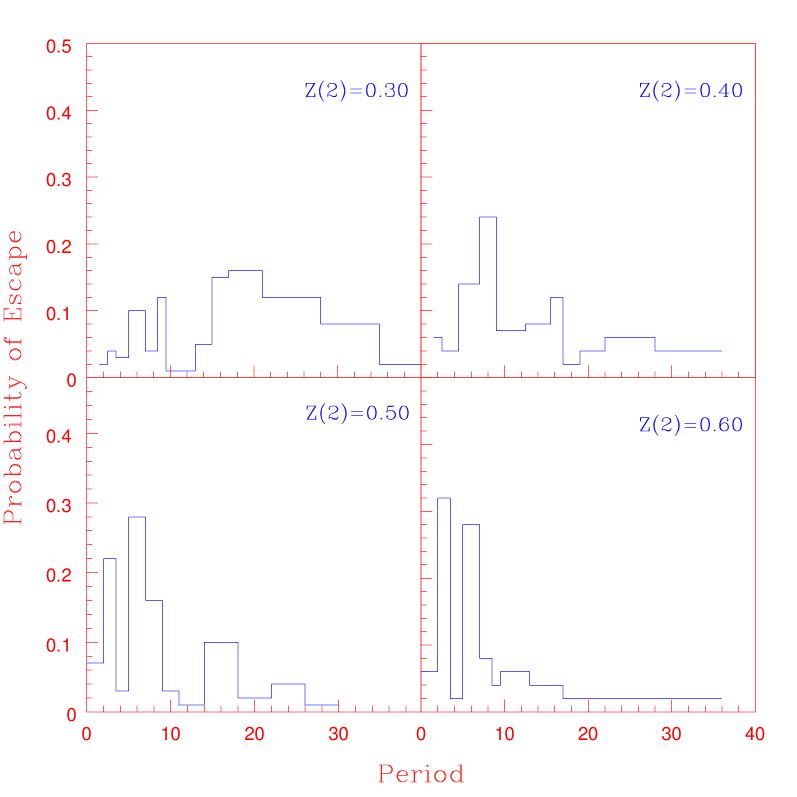
Figure 15: Escape probability as a function of different periods corresponding to four values of the signal amplitude of the high frequency $(\nu_{2}=0.32)$, showing VR for the low frequency signal $\nu_{1}$ for the cubic map in the threshold setup. Other parameters are $a=1.4,b=0.01$, $E=0.12$ and $Z(1)=0.16$.

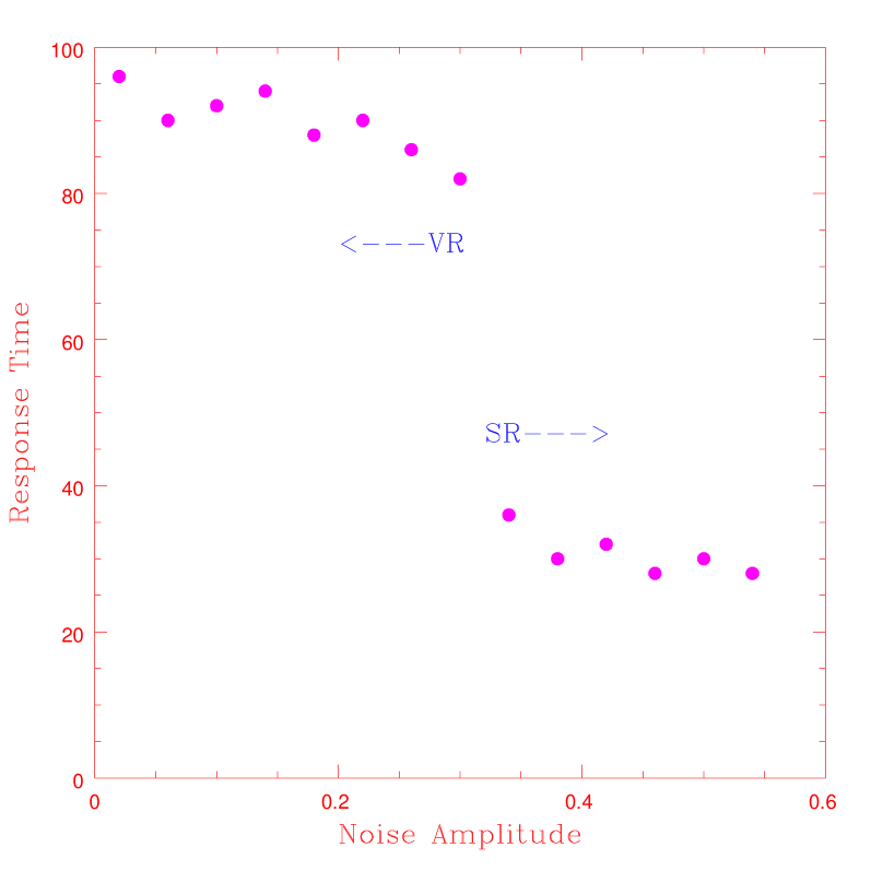
Figure 16: Variation of response time $\tau$ for VR and SR as a function of noise amplitude $E$, corresponding to the frequency $\nu_{1}=0.125$, for the cubic map in the threshold setup. For each $E$, the optimum value of the amplitude $Z(2)$ for the higher frequency $\nu_{2}=0.32$ is used. Two regions for VR and SR are clearly evident in terms of the response time.

6 Results and discussion

In this paper we undertake a detailed numerical study of SR and VR in a discrete model with a bichromatic input signal and gaussian noise. The model combines the features of bistable and threshold setups and turns out to be ideal for comparing various aspects of SR and VR. Both additive and multiplicative noise are used for driving the system in the bistable mode. To our knowledge, this is the first instance where VR has been explicitely shown in a discrete system.

The system shows bistability in periodic and chaotic attractors. Hence a subthreshold signal can be enhanced with the inherent chaos in the system in the absence of noise. With a composite input signal and noise, all the component frequencies are enhanced in the output at different optimum noise amplitudes.

Our analysis brings out some fundamental differences between the two mechanisms of SR with respect to amplification of multisignal inputs. In particular, we find that, while the bistable set up responds only to the fundamental frequencies present in the input signal, the threshold mechanism enhances a mixed mode also, a result not possible in the context of linear signal processing. This may have potential practical applications, especially in the study of neuronal mechanisms underlying the detection of pitch of complex tones [19,36].

Another especially interesting result we have obtained is regarding a cross over behavior between VR and SR in terms of an initial response time. The response time decreases sharply in going from VR to SR and depends only on the background noise level. In the regime of VR, the system shows the so called bona fide resonance, where the response becomes optimum for a narrow band of intermediate frequencies. Moreover, the optimum value of high frequency signal amplitude increases with frequency, but as the frequency increases beyond a limit, it becomes less effective in producing VR.

Finally, two other results obtained in the context of SR are the usefulness of a high frequency signal in enhancing the SNR of a low frequency signal and the possibility of using SR as a filter for the detection or selective transmission of fundamental frequencies in a composite signal using a bistable nonlinear medium. The former is evident from Fig.8 and shows certain cooperative behavior between the two signals. Similar results have been obtained earlier [20,37] under other specific dynamical setups, but the simplicity of our model suggests that the results could be true in general. The latter result arises due to the fact that the noise amplitudes for the optimum SNR for the two frequencies are different (see Fig.5 and Fig.8) and the difference $\Delta E$ tend to increase with the difference in frequencies $(|\nu_{1}-\nu_{2}|)$. This suggests that SR can, in principle, be used as an effective tool for signal detection/transmission in noisy environments. A similar idea has been proposed recently [18] in connection with the signal propogation along a one dimensional chain of coupled over damped oscillators. There it was shown that noise can be used to select the harmonic components propogated with higher efficiency along the chain.

- (1) L. Gammaitoni, P. Hanggi, P. Jung and F. Marchesoni, Rev.Mod.Phys. 70,223(1998).
- (2) P. Hanggi, ChemPhysChem 3,285(2002).
- (3) For other reviews, see: P. Jung, Phys.Rep. 234,175(1993); K. Wiesenfeld and F. Moss, Nature (London) 373,33(1995); K. Wiesenfeld and F. Jaramillo, CHAOS 8,539(1998); A. Bulsara and L. Gammaitoni, Phys.Today 49,39(1996); F. Moss and K. Wiesenfeld, Sci.Am. 273,50(1995).
- (4) R. Benzi, A. Sutera and A. Vulpiani, J.Phys. A 14,L453(1981).
- (5) C. Nicolis and G. Nicolis, Tellus 33,225(1981).
- (6) S. Mizutani, T. Sano, T. Uchiyama and N. Sonehara, IEICE Trans.Fund. E 82,671(1999); G. Balazsi, L. B. Kosh and F. E. Moss, CHAOS 11,563(2001); A. Ganopolski and S. Rahmstorf, Phys.Rev.Lett. 88,038501(2002).
- (7) J. C. Compte and S. Morfu, Phys.Lett. A 309,39(2003); S. Morfu, J. M. Bilbault and J. C. Compte, Int.J.Bif.Chaos 13,233(2003).
- (8) J. F. Lindner, B. K. Meadows, W. L. Ditto, M. E. Inchiosa and A. R. Bulsara, Phys.Rev.Lett. 75,3(1995); J. F. Lindner, S. Chandramouli, A. R. Bulsara, M. Locher and W. L. Ditto, Phys.Rev.Lett. 81,5048(1998); V. S. Anishchenko, M. A. Safanova and L. O. Chua, Int.J.Bif.Chaos 4,441(1994).
- (9) P. Landa and P. McClintock, J.Phys. A 33,L433(2000).
- (10) J. P. Baltanas, L. Lopez, I. I. Blechman, P. S. Landa, A. Zaikin, J. Kurths and M. A. F. Sanjuan, Phys.Rev. E 67,066119(2003).
- (11) A. A. Zaikin, L. Lopez, J. P. Baltanas, J. Kurths and M. A. F. Sanjuan, Phys.Rev. E 66,011106(2002).
- (12) V. M. Gandhimathi, S. Rajasekar and J. Kurths, Phys. Letters A 360,279(2006).
- (13) E. Ullner, A. Zaikin, J. Garcia-Ojalvo, R. Bascones and J. Kurths, Phys.Letters A 312,348(2003).
- (14) R. B. Mitson, Y. Simand and C. Goss, ICES J.Marine Sci. 53,209(1996); J. D. Victor and M. M. Conte, Visual Nuerosci. 17,959(2000).
- (15) D. Su, M. Chiu and C. Chen, Precis. Eng. 18,161(1996).
- (16) A. Maksimov, Ultrasonics 35,79(1997).
- (17) G. P. Agrawal, Fibre Optic Communication Systems, (John Wiley, New York, 1992).
- (18) A. A. Zaikin, D. Topaj and J. Garcia-Ojalvo, Fluct. Noise Lett. 2,L47(2002).
- (19) D. R. Chialvo, O. Calvo, D. L. Gonzalez, O. Piro and G. V. Savino, Phys.Rev. E 65,R050902(2002).
- (20) E. I. Volkov, E. Ullnev, A. A. Zaikin and J. Kurths, Phys.Rev. E 68,026214(2003).
- (21) K. P. Harikrishnan and G. Ambika, Physica Scripta 71,148(2005); K. P. Harikrishnan and G. Ambika, Proc.National Conf.Nonlinear Systems and Dynamics, (I.I.T.Kharagpur, 2003, p.261).
- (22) D. Cubero, J. P. Baltanas and J. Casado-Pascual, Phys.Rev. E 73,061102(2006); Y. C. Lai and K. Park, Math.Biosci.Engg. 3,583(2006).
- (23) Pu-Lin Gong and Jian-Xue Xu, Phys.Rev.E 63,031906(2001).
- (24) G. Ambika and N. V. Sujatha, Pramana-J.Phys. 54,751(2000).
- (25) G. Ambika, N. V. Sujatha and K. P. Harikrishnan, Pramana-J.Phys. 59,539(2002).
- (26) P. Hanggi and H. Thomas, Phys.Rep. 88,207(1982).
- (27) P. Jung and P. Hanggi, Phys.Rev. A 44,8032(1991).
- (28) M. I. Dykman, R. Mannella, P. V. E. McClinntock and N. G. Stocks, Phys.Rev.Lett. 68,2985(1992).
- (29) V. S. Anishchenko, A. B. Neiman, F. Moss and L. Schimansky-Geier, Physics-Uspekhi 42,7(1999).
- (30) R. Graham and A. Schenzle, Phys.Rev. A 25,1731(1982); D. S. Leonard and L. E. Reichl, Phys.Rev. E 49,1734(1994).
- (31) H. Risken, The Focker-Planck Equation, (Springer, Berlin, 1984).
- (32) G. Giacomelli, F. Marin and I. Rabbiosi, Phys.Rev.Lett. 82,675(1999).
- (33) V. N. Chizhevsky, E. Smeu and G. Giacomelli, Phys.Rev.Lett. 91,220602(2003).
- (34) M. Gitterman, J.Phys.A 34,L355(2001).
- (35) E. Lanzara, R. N. Montegna, B. Spagnolo and R. Zangara, Am.J.Phys. 65,341(1997).
- (36) J. F. Lindner, B. K. Meadows, T. L. Marsh, W. L. Ditto and A. L. Bulsara, Int.J.Bif.Chaos 8,767(1998).
- (37) M. E. Inchiosa, V. In, A. R. Bulsara, K. Wiesenfeld, T. Heath and M. H. Choi, Phys.Rev. E 63,066114(2001).