Genomes: at the edge of chaos with maximum information capacity

Abstract

We propose an order index, $\phi$, which quantifies the notion of “life at the edge of chaos” when applied to genome sequences. It maps genomes to a number from 0 (random and of infinite length) to 1 (fully ordered) and applies regardless of sequence length. The 786 complete genomic sequences in GenBank were found to have $\phi$ values in a very narrow range, 0.037$\pm$0.027. We show this implies that genomes are halfway towards being completely random, namely, at the edge of chaos. We argue that this narrow range represents the neighborhood of a fixed-point in the space of sequences, and genomes are driven there by the dynamics of a robust, predominantly neutral evolution process.

The Edge of chaos originally refers to the state of a computational system, such as cellular automata, when it is close to a transition to chaos, and gains the ability for complex information processing Langton90 ; Crutchfield90 ; Mitchell93 . The notion has since been used to describe biological states, and life in general, on the assumption that life necessarily involves complex computation Kauffman94 . In model systems such as cellular automata, there are well defined procedures for recognizing the change in computational cab ability during the transition from non-chaotic to chaotic states Langton90 ; Mitchell93 . However, these have not been adapted to the wider biological context, even for the simplest of organisms. But if we represent a living organism by its genome, view evolution as a dynamical process that drives genomes in the space of sequences, and consider chaos as a state of genome randomness, then we have a framework within which the meaning of “life occurs at the edge of chaos” may be investigated. Genomes, linear sequences written in the four chemical letters, or bases, A (adenine), C (cytosine), G (guanine) and T (thymine) and often referred to as books of life, regulate the functioning of organisms through the many kinds of codes embedded in them (there are also non-textual post-translational regulations; see, e.g. Davies00 ). When genomes are seen as texts, they have several key properties reflecting their complexity, including long-range correlations and scale invariance Li92 ; Peng92 ; Voss92 (although this topic is debated Israeloff96 ), self-similarity Church93 ; Lu98 ; Nagai01 ; Chen05b , and distinctive Shannon redundancy Mantegna94 ; Stanley99 ; Chen05 . However, these properties do not give a measure of the proximity of a genome to chaos or randomness. Before the edge-of-chaos notion can be explored, one needs to have a quantity that measures the randomness of genomes as texts.

Here we analyze genomes in terms of the frequency of occurrence of $k$-letter words, called $k$-mers, where $k$ is a small integer Hao00 . For a given $k$, the $4^{k}$ types of $k$-mers are partitioned into $k$+1 “$m$-sets”, $m$=0–$k$. An $m$-set is composed of all the $k$-mers containing $m$ and only $m$ A or T’s. There are $\tau_{m}$=$2^{k}$${\left(\begin{matrix}k\cr m\cr\end{matrix}\right)}$ types of $k$-mers in an $m$-set. The reason for partitioning the $k$-mers according to AT-content for statistical purposes is that although the A:T and C:G ratios are invariably close to 1, Prabhu93 ; Mrazek98 ; Bell99 , the AT to GC ratio may differ significantly. This partition is needed for preventing biased base composition from masking crucial statistical information in genomes Israeloff96 ; Chen05 . For $k$$\geq$2, the $k^{th}$ order index for a sequence of length $L$ (in bases) is

$$\phi\equiv{1\over(2-2(p^{k}+q^{k}))}\sum_{m}{1\over L}\left|L_{m}-L^{\{\infty\}}_{m}\right|,$$ (1)

where 0$<$$p$$<$1 is the fractional AT-content in the sequence; $q$=1-$p$; $L_{m}$ is the total number of $k$-mers in the $m$-set; and $L^{\{\infty\}}_{m}$ is the expected value for $L_{m}$ in a $p$-valued random sequence of infinite length: $L^{\{\infty\}}_{m}$=$L$$2^{-k}$ $\tau_{m}$$p^{m}$$q$^k-m. The definition of $\phi$ is based on the observation that distribution-averages are useful indicators of the randomness of a sequence. The denominator on the right-hand-side of Eq. (1) is a normalization factor which ensures $\phi$$\approx$1 for an ordered sequence (in which all AT’s are on, say, the 5’ end and all CG’s are on the 3’ end). The singularities at $p$= 0 and 1 are not a practical problem since no genome has such extreme base composition.

From the central limit theory we expect, for random sequences, $|L_{m}-L^{\{\infty\}}_{m}|$ to scale as $L_{m}^{-1/2}$. We therefore expect $\phi$ to be proportional to $L^{-1/2}$ on average.

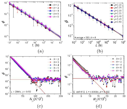
Figure 1: (a) Log-log plot of order index, $\phi$, vs. length of random sequence for $p$=0.5 and $k$=2–6. (b) Same as (a); for $k$=4 and $p$=0.20–0.50. (c) Semi-log plot of $\phi$ vs. $N_{\mu}$, number of random point mutations, for an initially ordered 20 Mb, $p$=0.5 sequence. The intersection of the red lines is the critical point where sequence becomes random. (d) Same as (c); initial sequence is genome of E. coli.

The log-log plots in Fig. 1 (a) and (b) show $\phi$ as a function of sequence length for different $k$’s and $p$’s. Each datum is averaged over 500 random sequences. It is seen that $\phi$ scales very well as $L^{-1/2}$ (with sizable fluctuations), and is only weakly dependent on $k$ and $p$. These results can be summarized for all $k$ and $p$ by an empirical relation:

$$\phi^{\{ran\}}=c_{\phi}L^{-\gamma_{\phi}}$$ (2)

with $\gamma_{\phi}=0.50\pm 0.01$ and $c_{\phi}=1.0\pm 0.2$ or, to a good approximation, $\phi^{\{ran\}}$$\approx$$L^{-1/2}$. This leads to the convenient concept of an equivalent length for a $\phi$-value sequence, $L_{eq}(\phi)$$\equiv$$\phi^{-2}$, the nominal length of a random sequence whose order index is $\phi$.

Random events such as point mutations acting on a non-random sequence decreases its order, and hence its $\phi$. Fig. 1 (c) shows that the $\phi$ of a $p$=0.5, 20 Mb ordered sequence, decreases exponentially with the number of mutations $N_{\mu}$, until $N_{\mu}$ reaches a critical number $N_{\mu c}$. The critical value reflects the fact that a random sequence does not become more random with further changes. In other words, if one thinks of random point mutation as a dynamical action taking a sequence from one point in the sequence space to another, then a randomized sequence is a fixed-point of the action. Our studies of initially ordered sequences having a variety of lengths and base compositions yield,

$$\phi={\left\{\begin{matrix}\exp{(-2N_{\mu}/L)},\ N_{\mu}\lesssim N_{\mu c};\cr\phi_{c}\approx L^{-1/2},\quad N_{\mu}>N_{\mu c}\cr\end{matrix}\right.}$$ (3)

where the $N_{\mu c}$$\approx$(1/4)$L\ln L$, and the critical mutation rate is $\mu_{c}$$\equiv$$N_{\mu c}/L$$\approx$(1/4)$\ln L$. The formula for $N_{\mu c}$ compares well with simulation. In the case of Fig. 1 (c), the coordinates of the simulation ($k$=4) critical point are ($\phi_{c}$, $N_{\mu c}$)=(2.2$\times$$10^{-4}$, 8.5$\times$$10^{7}$), as compared to the “theoretical” values (2.2$\times$$10^{-4}$, 8.4$\times$$10^{7}$). For typical sequences of genomic length ($L$$\sim$10^1±1 Mb), $\mu_{c}$=4.0$\pm$0.6 mutations per base (b^-1). We use Eq. (3) to assign to a $\phi$-valued sequence an equivalent mutation rate, $\mu_{eq}(\phi)$$\equiv$$\ln\phi^{-1/2}$, the nominal number of random point mutations per base required to bring the index of an ordered sequence to $\phi$.

Eq. (3) can be adapted for application to sequences not initially ordered. For example, the equivalent mutation rate for the 4.6 Mb genome of E. coli ($\phi$=0.049) is 1.5 b^-1. Since for a 4.6 Mb sequence $\mu_{c}$=3.8 b^-1, one expects an additional 2.3$\times$4.6$\times$10⁶= 1.1$\times$10⁷ mutations are needed to randomize it. In the simulation shown in Fig. 1 (d), the actual number needed is found to be (1.1$\pm$0.1)$\times$10⁷.

We computed $\phi$ for 384 complete prokaryotic genomes (28 archaebacteria and 356 eubacteria) and 402 complete chromosomes from 28 eukaryotes of lengths ranging from 200 kb to 230 Mb. The rice genome was downloaded from the Rice Annotation Project Database rice , and all other sequences from the National Center for Biotechnology Information genome database NCBI , during the period 26 Feb.–27 Nov., 2006. The 28 eukaryotes (number of chromosomes and genome length in parenthesis) include 11 fungi, A. fumigatus (8, 28.8 Mb), C. albicans (1, 0.95 Mb), C. glabrata (13, 12.3 Mb), C. neoformans (14, 19.1 Mb), D. hansenii (7, 12.2 Mb), E. cuniculi (11, 2.50 Mb), E. gossypii (7, 8.74 Mb), K. lactis (6, 10.7 Mb), S. cerevisiae (Yeast) (16, 12.1 Mb), S. pombe (Fission Yeast) (3, 10.0 Mb), Y. lipolytica (6, 20.5 Mb); the unicellular P. falciparum (Malaria) (14, 22.9 Mb); 2 plants, A. thaliana (Mustard) (5, 119 Mb), O. sativa (Rice) (12, 372 Mb); 5 insects, C. elegans (Worm) (6, 100 Mb), D. melanogaster (Fly) (6, 118 Mb), A. gambiae (Mosquito) (5, 223 Mb), A. mellifera (Bee) (16, 183 Mb), T. castaneum (Beetle) (10, 112 Mb); 9 vertebrates, D. rerio (Zebrafish) (25, 1.04 Gb), G. gallus (Chicken) (30, 933 Mb), B. taurus (Cow) (30, 1.41 Gb), C. familiaris (Dog) (39, 2.31 Gb), M. musculus (Mouse) (21, 2.57 Gb), R. norvegicus (Rat) (21, 2.50 Gb), M. mulatta (Monkey) (21, 2.73 Gb), P. troglodytes (Chimpanzee) (25, 2.86 Gb), H. sapiens (Human) (24, 2.87 Gb).

The results shown in Fig. 2 indicate that genomic $\phi$’s systematically vary neither with sequence length ((a) and (b)),

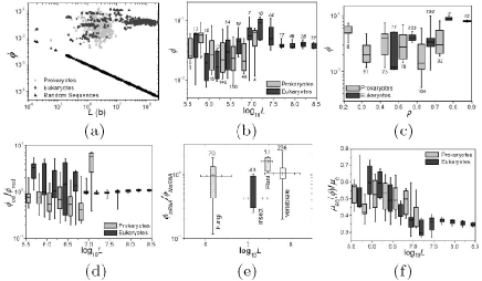
Figure 2: (a) Order index, $\phi$, vs. sequence length, $L$, for 384 prokaryotic genomes (gray  ’s), 402 eukaryotic chromosomes (black $\bullet$’s), and random sequences (line composed of $\bigtriangledown$’s). In (b–f): Box (gray for prokaryotes; black for eukaryotes) height is given by 25% to 50% values and the range represents 10% to 90% values; numbers above boxes are numbers of sequences in group; all $\phi$’s are averaged over $k$=2 to 6. (b) $\phi$ vs. $\log L$. (c) $\phi$ vs. fractional AT-content, $p$. (d) Ratio of $\phi_{cd}$ (for coding parts) to $\phi_{ncd}$ (noncoding) vs. $\log L$. (e) Ratio of $\phi_{mRNA}$ (mRNA segments) to $\phi_{nmRNA}$ (non-mRNA), averaged over classes of eukaryotes. (f) Ratio of equivalent mutation rate, $\mu_{eq}$, to critical mutation rate, $\mu_{c}$, vs. $\log L$.

nor with base composition ((c)). Instead they have a nearly universal value — the average over all sequences is $\phi_{g}$$\equiv$0.037$\pm$0.027 (this defines the symbol $\phi_{g}$). We have verified that, as a general rule, within a genome the variation in segmental $\phi$ decreases with segmental length and the average $\phi$ reaches its whole-genome value when the size of the segment exceeds 50 kb. In Fig. 2 (a) the spread in $\phi$ of the genomic data shows a tendency to decrease with sequence length. Part of this effect may be purely statistical: smaller sample sizes (i.e., sequence lengths) tend to have larger statistical fluctuations. Part of it may also be because sequences longer than 10 Mb are all from chromosomes of multicellular eukaryotes that are phylogenetically close. In any case Fig. 2 (a) clearly puts the genomes in a category apart from random sequences.

From each complete sequence, we extracted the coding and noncoding parts (owing to imperfect annotation, the sum of the parts sometimes differ slightly from the whole), then concatenated the parts into two separate sequences and computed their order indexes, $\phi_{cd}$ and $\phi_{ncd}$, respectively. A summary of the ratio $\phi_{cd}/\phi_{ncd}$ for sets of genomes grouped by length is given in Fig. 2 (d). For prokaryotes the ratio ranges (10^th to 90^th percentile) from 0.15 to 3 with a median of about 0.5. Notable exceptions are the three bacteria with exceptionally large genomes ($L$$\lesssim$10 Mb) with ratios ranging from 5 to 7: S. avermitilis, S. coelicolor, and Mycobacterium sp. MCS.

For the eukaryotic chromosomes longer than 10 Mb the ratios do not significantly deviate from unity. Mustard, whose coding and noncoding parts have nearly equal lengths ($\sim$10–12 Mb), is the only exception in this category with $\phi_{cd}/\phi_{ncd}$$\approx$7 (these ratios are beyond the 90 percentile and therefore are not included in Fig. 2 (d)). In this case $\phi_{cd}$$\approx$0.055 is similar to other genomes while $\phi_{ncd}$$\approx$0.0075 is about seven times less than the norm. Rice, the only other plant included in this study, with $\phi_{cd}/\phi_{ncd}$$\approx$0.35 is unlike mustard but more like the other eukaryotes. For the eukaryotic chromosomes shorter than 10 Mb the ratios average to about 2 but show greater variation.

The coding parts of eukaryotic genomes are further partitioned into mRNA and non-mRNA parts, and their $\phi$’s computed separately. Averaged over sets of organisms, $\phi_{mRNA}/\phi_{nmRNA}$ is of the order of 1, with the ratio being $\sim$0.5 for insects and $\sim$2 for plants (Fig. 2 (e)). For the latter, the ratio is $\sim$1 for the five chromosomes of mustard and $\sim$2 for the twelve chromosomes of rice. In summary, the differences in $\phi$ between coding and non-coding parts, and between mRNA and non-mRNA parts are much smaller than the difference between genomes and random sequences.

The ratio $\mu_{eq}(\phi)$/$\mu_{c}$ is an indication of how close a sequence is to being random. Fig. 2 (f) shows that the shorter ($L$$\gtrsim$10 Mb) sequences are roughly half-way, and the longer sequences, one-third of the way, towards becoming random. The systematic but weak length-dependence of the ratio is explained by the fact that the genomic $\phi$, hence $\mu_{eq}(\phi)$, is approximately constant, whereas $\mu_{c}$ is proportional to $\ln L$. The overall average of the ratio is 0.45$\pm$0.11.

We summarize our results by considering the function

$$I(z)=-z\ln z-(1-z)\ln(1-z)$$ (4)

where $z$=$\phi^{\lambda}$ and $\lambda$=0.21. The value of the exponent $\lambda$ is determined by requiring that $z$=0.5 at $\phi$=$\phi_{g}$. $I(z)$ is the simplest function that maps the range (0,1) to a positive real value, has zeros at (and only at) $z$=0 and 1, has a maximum at $z$=0.5 and is symmetric with respect to the point $z$=0.5. In Fig. 3 the parabola-like curve shows $I(z)$ plotted against $z$. In addition, three other sets of abscissas are given: $\phi$; $\log_{10}L_{eq}(\phi)$, where $L_{eq}(\phi)$ is the equivalent length (Eq. (2)); and $\mu_{eq}(\phi)$, the equivalent mutation rate. A scale linear in $z$, relative to one in $\phi$, is a better representation of the space of possible sequence lengths.

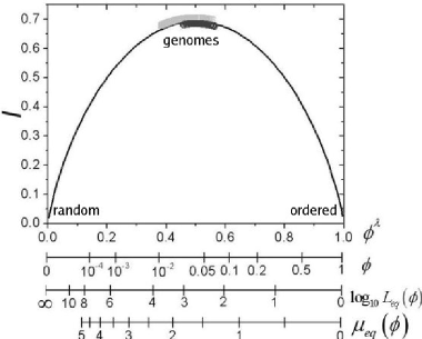
Figure 3: The function $I(z)$ (Eq. (4)) plotted as a function of: $z$=$\phi^{\lambda}$ ($\lambda$=0.21); $\phi$; $\log_{10}L_{eq}(\phi)$ (Eq. (2)); $\mu_{eq}(\phi)$ (in units of b^-1; Eq. (3)). Data from prokaryotic (gray) and eukaryotic (black) genomes occur near the peak of $I$ and have $\phi$$\sim$$\phi_{g}$, $L_{eq}$$\sim$.25–10 kb, and $\mu_{eq}$$\sim$1.8$\pm$0.5 b^-1.

It is seen in Fig. 3 that genomes are concentrated near the peak of the $I$-curve and equally and far removed from the random ($z$$\sim$0) and ordered ($z$$\sim$1) sequences.

The genomic equivalent lengths, occupying a small neighborhood around at $L_{eq}(\phi_{g})$=730 b, are far shorter than the actual lengths of complete sequences. Among the many possible mechanisms that may cause long sequences to have short equivalent lengths, by far the simplest is replication. This is because a long sequence of length $L$ composed of multiple replications of a random sequence $l$ bases long will have $L_{eq}$$\sim$$l$, independent of $L$. Similarly, if genome growth is dominated by random segmental duplication Lynch02 ; Bailey02 ; Zhang05 , then the genomic $L_{eq}$ will be much shorter genome length Chen05 .

The genomic equivalent mutation rates span a small range around 1.8 b^-1, or about 45% of the critical mutation rate of approximately 4 b^-1 that would randomize the genomes. Thus, for example, a typical worm (C. elegans) chromosome, with an average length of 17 Mb and an equivalent mutation rate of 1.8 b^-1, is as random as an initially ordered 17 Mb sequence after having undergone 31 million random mutations - as compared to the 68 million mutations which would randomize the sequence. In this sense genomes are quasi-random - or “at the edge of chaos”. For a linear text, quasi-randomness satisfies two crucial necessary conditions for high information content: high efficiency and large variation in word usage. A random sequence has maximum word-usage efficiency because all its $k$-mers in an $m$-set have occurrence frequencies very close to the theoretical mean frequency of the set, $\bar{f}^{\{\infty\}}_{m}$=$L^{\{\infty\}}_{m}$/$\tau_{m}$. However, this also implies minimum word-usage variation, which prevents a random sequence from being information-rich. In a quasi-random sequence a compromise between high efficiency and large variation in word usage is obtained by suitably relaxing the equal-frequency condition Chen05 , thus allowing a genome at the edge of chaos to have close to maximum information capacity.

The high concentration of genomic $\phi$’s near $\phi_{g}$ may be interpreted as the signature of a certain robust characteristics in the genomic evolution processes. The near equality of $\phi$’s for coding and noncoding regions within a genome suggests that the underlying evolution processes are not dominated by codon selection, but are likely predominantly selectively neutral Kimura80 ; Fu93 . We therefore propose the following conjecture: Just as randomness is a fixed-point of the action of random point mutations, the state of genomes defined by $\phi$$\sim$$\phi_{g}$ is a fixed-point of the action of a robust, predominantly neutral evolution process. The observed shortness of $L_{eq}(\phi_{g})$ suggests that the neutral process is dominated by (non-deleterious) random segmental duplications Lynch02 ; Bailey02 ; Zhang05 , occurring singly Chen05 ; Hsieh03 and in tandem Messer05 . We consider random segmental duplication to be an infrastructure-building process because it does not necessarily produce information directly. Instead, it causes genomic $\phi$ to be close to $\phi_{g}$, giving genomes maximum information capacity. Since this enhances genomic fitness indirectly, the neutral process may in itself be a product of natural selection. The near randomness of the neutral process guarantees the fixed-point associated with $\phi_{g}$ to have a very large configuration space, hence relatively low free energy, thus rendering $\phi_{g}$-valued states widely accessible. In contrast, non-neutral, information-gathering processes dominated by selection (narrowly construed) are predominantly point mutations: they are poor mechanisms for inducing genomic states of maximum capacity, and do not lead to widely accessible states. Taken together these suggest that the evolution of the genome may have been driven by a two-stage process: one neutral, robust, infrastructure-building and universal, and the other selective, fine-tuning, information-gathering and diverse. An example of such a two-step process is found in the paradigm of accidental gene duplication followed by mutation driven subfunctionalization Lynch00 ; Zhang03 . We may assume that during the long history of the genome’s growth and evolution, the twin-processes acted in a ratchet-like, complementary manner, driving the genome, in successive stages, to a state of maximum information capacity, and helping it to acquire, at each stage, near-maximum information content.

This work is supported in part by grant nos. 95-2311-B-008-001 and 95-2911-I-008-004 from the National Science Council (ROC).

References

- (1) C. G. Langton. Physica D 42, 12-37 (1990).
- (2) J. P. Crutchfield and K. Young. In W. H. Zurek, editor, Complexity, entropy, and the physics of information, 223-269 (Addison-Wesley, Redwood City, CA, 1990).
- (3) M. Mitchell, P. T. Hraber, and J. P. Crutchfeld. Complex Systems, 7, 89-130 (1993).
- (4) S. A. Kauffman. (Oxford Univ. Press, London, 1993).
- (5) S. P. Davies, et al. Biochem. J. 351, 95-105 (2000).
- (6) W. Li and K. Kaneko. Europhys. Lett. 17, 655-660 (1992).
- (7) C. K. Peng, et al. Nature 356, 168-170 (1992); Phys. Rev. E 47, 3730-3733 (1993).
- (8) R. F. Voss. Phys. Rev. Lett. 68, 3805-3808 (1992).
- (9) N. E. Israeloff, et al. Phys. Rev. Lett. 76, p1976 (1996); S. Bonhoeffer, et al. loc. cit. p1977; R. F. Voss. loc. cit. p1978; N. Mantegna, et al. loc. cit. p1979. Also: C. A. Chatzidimitriou-Dreismann, et al. NAR 24, 1676-1682 (1996).
- (10) K. W. Church, J. I. Helfman, J. Comp. Graph. Stat. 2, 153-174 (1993).
- (11) X. Lu, Z. Sun, H. Chen, Y. Li. Phys. Rev. E 58, 3578-3584 (1998).
- (12) N. Nagai. Jpn J Physiol. 51, 159-68 (2001).
- (13) T. Y. Chen, L. C. Hsieh and H. C. Lee. Comp. Phys. Comm. 169, 218-221 (2005).
- (14) R..N. Mantegna, et al. Phys. Rev. Lett. 73, 3169-3172 (1994); Phys. Rev. E 52, 2939-2950 (1995).
- (15) H. E. Stanley, et al. Physica A 273, 1-18 (1999).
- (16) H. D. Chen, et al. Phys. Rev. Lett. 94 178103 (2005).
- (17) B. L. Hao, H. C. Lee and S. Y. Zhang. Chaos Solitons Fract. 11, 825-836 (2000).
- (18) V. V. Prabhu Nucl. Acids Res. 21, 2797-2800 (1993).
- (19) J. Mrazek and S. Karlin. Proc. Nat. Acad. Sci. (USA) 95 3720-3725 (1998).
- (20) S. J. Bell and D. R. Forsdyke J. theor. Biol. 197, 51-61 (1999).
- (21) Rice Annotation Project Database; http://rapdb.lab.nig. ac.jp/ (Nov. 2006).
- (22) National Center for Biotechnology Information genome database; http://www.ncbi.nlm.nih.gov/ (Oct. 2006).
- (23) M. Lynch. Science 297 945-947 (2002).
- (24) J. A. Bailey, et al. Science 297, 1003-1007 (2002).
- (25) L. Zhang, et al. Mol. Bio. Evol. 22 135-141 (2005).
- (26) M. Kimura. J. Mol. Evol. 16 111-120 (1980).
- (27) Y. X. Fu and W. H. Li. Genetics 133 693-709 ( 1993).
- (28) L. S. Hsieh, L. F. Luo, F. M. Ji and H. C. Lee. Phys. Rev. Lett. 90 018101 (2003).
- (29) P. W. Messer, P. F. Arndt, and M. Laessig. Phys. Rev. Lett. 94 138103 (2005).
- (30) M. Lynch and J. S. Conery. Science 290 1151-1155 (2000).
- (31) J. Zhang. Trends Eco. Evol. 18, 292-298 (2003).