Scattered Emission from A Relativistic Outflow and Its Application to Gamma-Ray Bursts

Abstract

We investigate a scenario of photons scattering by electrons within a relativistic outflow. The outflow is composed of discrete shells with different speeds. One shell emits radiation for a short duration. Some of this radiation is scattered by the shell(s) behind. We calculate in a simple two-shell model the observed scattered flux density as a function of the observed primary flux density, the normalized arrival time delay between the two emission components, the Lorentz factor ratio of the two shells and the scattering shell’s optical depth. Thomson scattering in a cold shell and inverse Compton scattering in a hot shell are both considered. The results of our calculations are applied to the Gamma-Ray Bursts and the afterglows. We find that the scattered flux from a cold slower shell is small and likely to be detected only for those bursts with very weak afterglows. A hot scattering shell could give rise to a scattered emission as bright as the X-ray shallow decay component detected in many bursts, on a condition that the isotropically equivalent total energy carried by the hot electrons is large, $\sim 10^{52-56}$ erg. The scattered emission from a faster shell could appear as a late short $\gamma$-ray/MeV flash or become part of the prompt emission depending on the delay of the ejection of the shell.

1 Introduction

Gamma-Ray Bursts (GRBs) are a cosmological phenomenon with a huge energy release, fast variabilities and very complex multi-wavelength light curves. A relativistic outflow is unavoidable in order to explain the fast variability and so called “compactness problem” (see Piran 2005 for a review). According to the standard “Fireball” model, the outflow from the GRB central engine has a finite duration and can have a wide range in its velocities, thus can be modeled by being made of discrete relativistic shells. These shells are responsible for the observed $\gamma$-rays (via internal shocks) and for the afterglow emissions (via external shocks) (cf. Piran 2005). In this picture, if one shell emits $\gamma$-rays, some fraction of that emission should be scattered by shells behind, and the scattered emission would arrive at the observer at a different time, with a different flux and possibly at a different photon frequency. Detection of the scattered photons would help us explore the properties of the GRB ejecta and the late outflow.

In the present paper we consider a simple scenario, where only two consecutive shells are present: one shell radiates and the other receives some of this radiation and scatters it. The two shells can have different speeds and the shell that receives and scatters the emission can have an arbitrarily large time delay in its ejection from the central source, but it has to be behind the emitting shell. An observer detects the primary emission from the first shell and then the scattered emission from the second one at a later time because of the light-travel time. We calculate the ratio between these two emissions’ fluxes, the time delay in their arrival, the ratio between their frequencies and the ratio between their durations.

Early GRB X-ray observations by Swift have shown a “canonical” behavior that presents a puzzling shallow decay typically lasting for a few hours (e.g. Nousek et al. 2006). This decay phase is poorly understood (see Zhang 2007 for a review of current possible models). We will explore the possibility that this shallower decay could be due to the scattered emission.

The scattering of the GRB prompt emission photons by electrons or dust grains in a dense circum-burst environment has been investigated before (e.g., Esin & Blandford 2000; Madau et al. 2000; Shao & Dai 2007; Heng et al. 2007). The scattering process we consider in this work happens within the GRB outflows, which is a natural outcome of the outflow when it has a finite duration and a variable speed.

The paper is structured as follows. We first derive a general formula for the observed flux from a relativistic shell in §2. In §3 we construct the flux and geometrical relations for a two-shell model. The formulae for the scattering process are developed in §4. Then we elaborate the primary and scattered emission relations such as time delay, frequency ratio and time duration ratio in §5. We present the main result - the ratio between the scattered and the primary fluxes - in §6. The application to the GRB shallower decay data is presented in §7. A faster scattering shell case is discussed in §8. We also discuss X-ray dim bursts and X-ray-dark short bursts, for which the scattered emission might be easier to detect, in §9. Finally, the summary and conclusions are given in §10.

2 Emission from a relativistic shell

Consider a spherical shell moving relativistically with Lorentz factor (LF) $\Gamma$ (when the shell is beamed with an opening angle $\geq\Gamma^{-1}$, it still can be considered as being spherical). The surface brightness in the rest frame of the shell is $\epsilon^{\prime}_{\nu^{\prime}}$ (erg s^-1 cm^-2 Hz^-1 sr^-1), the luminosity distance between the observer and the shell is $D_{L}$ and the radius of the shell is $R$, both of these distances measured in the laboratory frame. The flux density received at a frequency $\nu$ by the observer ahead of the shell, $f_{\nu}$, can be obtained by calculating the specific luminosity of the relativistic shell. The luminosity of the shell is given by $f_{\nu}(4\pi D_{L}^{2})=\epsilon^{\prime}_{\nu^{\prime}}(4\pi R^{2})\Gamma(2\pi)$. The last expression includes a factor of $\Gamma$, to take into account the “boost” that the photons experience; and a factor of $2\pi$, since we assume that the photons are being emitted isotropically from the shell, in the rest frame of the shell, and we are only interested in the ones reaching the observer. The two expressions yield

$$f_{\nu}=2\pi\epsilon^{\prime}_{\nu^{\prime}}\Gamma\biggl{(}\frac{R}{D_{L}}\biggr{)}^{2}.$$ (1)

3 Two shells scenario

Consider now two thin shells being ejected with an half opening angle of $\theta_{j}$ from the central engine. Shell 1 is ejected first with LF $\Gamma_{1}$ and, after a delay $\delta t$, measured in the laboratory frame, shell 2 is ejected with LF $\Gamma_{2}$. We assume that shell 1 is emitting photons isotropically in its co-moving frame and is characterized by an angular-independent surface brightness, $\epsilon^{\prime}_{\nu^{\prime}}$, on both sides of the shell. In the laboratory frame most of these photons will appear to move in the same direction as shell 1 and reach a distant observer, and a few will move in the opposite direction, encountering shell 2 on their way. These photons will be scattered by shell 2 and then reach the observer. See Figure 1 for an illustration. We will use primed quantities to specify the co-moving frame where the quantity is being measured: unprimed corresponds to the laboratory frame, primed (^′) to the co-moving frame of shell 1, and double primed (^′′) to the co-moving frame of shell 2.

Before proceeding with the detailed calculations about the scattered emission, we provide simple scaling relationships between the observed scattered emission and the observed direct emission from shell 1 by only considering the line-of-sight region.

Let us assume $\nu$ is the photon frequency of the direct emission from shell 1. In the shell 1 co-moving frame, the emitted photon frequency is $\nu^{\prime}\simeq\frac{\nu}{\Gamma_{1}}$ due to the relativistic Doppler effect (for simplicity we neglect the factor of 2). As seen by shell 2 the photon has a frequency of $\nu^{\prime\prime}\simeq\nu^{\prime}\frac{\Gamma_{2}}{\Gamma_{1}}$. If shell 2 is cold, the scattering does not change the photon’s energy. The observed frequency of the scattered emission is $\nu_{s}\simeq\nu^{\prime\prime}\Gamma_{2}$. Thus the observed frequency ratio between the two emissions is $\frac{\nu_{s}}{\nu}\simeq(\frac{\Gamma_{2}}{\Gamma_{1}})^{2}$.

The scattered emission will be observed at a later time, because the scattered photon has traveled an extra distance. This extra distance is equal to $R_{1}(1-\frac{\beta_{2}}{\beta_{1}})+\beta_{2}\delta t$, where $R_{1}$ is the distance of shell 1 from the central engine when a photon was emitted from shell 1 toward shell 2, and $\beta_{1}$ and $\beta_{2}$ are shell 1 and shell 2 velocities, respectively (the first part of the expression is due to the difference in the speeds of the shells, and the second part is due to the ejection delay of shell 2). The observed delay of the scattered emission is this separation divided by the speed of light $\approx\frac{R_{1}}{2\Gamma_{2}^{2}c}\approx T(\frac{\Gamma_{1}}{\Gamma_{2}})^{2}$ for small $\delta t$, where $T$ is the observed time of the shell 1 direct emission since the central engine explosion.

If $L$ is the luminosity observed directly from shell 1, the shell 1 co-moving frame luminosity would be $L^{\prime}\simeq\frac{L}{\Gamma_{1}^{2}}$. In the shell 2 co-moving frame, shell 1 has a luminosity of $L^{\prime\prime}$. Using the Lorentz invariance of $I_{\nu}/\nu^{3}$ we find that the luminosity ratio, $\frac{L^{\prime\prime}}{L^{\prime}}$, is the frequency ratio to the fourth power, or $\frac{L^{\prime\prime}}{L^{\prime}}\simeq(\frac{\nu^{\prime\prime}}{\nu^{\prime}})^{4}\simeq(\frac{\Gamma_{2}}{\Gamma_{1}})^{4}$. In the shell 2 co-moving frame, $\tau_{e}L^{\prime\prime}$ is the luminosity of the scattered emission, where $\tau_{e}$ ($<1$) is the shell 2 electron’s optical depth. Then the observed luminosity of the scattered emission is $L_{s}\simeq\tau_{e}L^{\prime\prime}\Gamma_{2}^{2}$. Thus we obtain that $\frac{L_{s}}{L}\simeq\tau_{e}(\frac{\Gamma_{2}}{\Gamma_{1}})^{6}$, which shows that the observed luminosity ratio is strongly dependent on the LF ratio. Since $\frac{\nu_{s}}{\nu}\simeq(\frac{\Gamma_{2}}{\Gamma_{1}})^{2}$, this indicates that the observed specific flux ratio is $\frac{f_{\nu,s}^{s}}{f_{\nu}}\simeq\tau_{e}(\frac{\Gamma_{2}}{\Gamma_{1}})^{4}$.

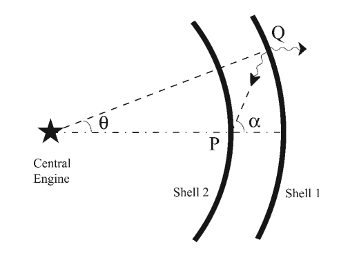
Figure 1: A simple two-shell scenario geometry. The diagram shows two photons emitted at the same time from point $Q$ on shell 1. One photon travels to the observer ahead of shell 1, while the other travels back to point $P$ on shell 2. Note that the figure shows shell 1 and the photons at time $t$ and shell 2 at time $t+l$, where $l$ is the light travel time from $Q$ to $P$.

3.1 Incident flux on shell 2

Now we work on the calculation of the scattered flux on more detail. In order to determine the scattered flux from shell 2 we will first calculate the incident flux from shell 1 at the point of shell 2 that intersects the line of sight between the central engine and the observer - we will call this point $P$. To do this, we will use the Lorentz invariance of $I_{\nu}/\nu^{3}$, where $I_{\nu}$ (erg s^-1 cm^-2 Hz^-1 sr^-1) is the specific intensity and $\nu$ is the frequency of the photon.

Let us consider a bundle of rays being emitted at an arbitrary point - $Q$ - on shell 1 and directed to the point $P$ (see Figure 1). The angle between the line of sight and the line connecting the central engine and $Q$ is $\theta$. The angle between the line of sight and the line connecting $P$ and $Q$ is $\alpha$. From the Lorentz invariance of $I_{\nu}/\nu^{3}$ we can obtain the relation

$$\frac{I_{\nu}}{I^{\prime\prime}_{\nu^{\prime\prime}}}=\biggl{[}\frac{1}{\Gamma_{2}(1+\beta_{2}\cos\alpha)}\biggr{]}^{3},$$ (2)

where $I_{\nu}$ is the specific intensity of the bundle of rays measured by an observer standing still in the laboratory frame and at the position of point $P$ (note that $I_{\nu}$ is NOT the specific intensity of the emission detected by a distant laboratory-frame observer sitting in front of shell 1); $I^{\prime\prime}_{\nu^{\prime\prime}}$ is the specific intensity of the bundle of rays measured in the shell 2 co-moving frame at point $P$. We can relate $I_{\nu}$ with the specific intensity of the bundle of rays measured in the shell 1 co-moving frame at point $Q$, $I^{\prime}_{\nu^{\prime}}$, as follows

$$\frac{I_{\nu}}{I^{\prime}_{\nu^{\prime}}}=\biggl{\{}\frac{1}{\Gamma_{1}[1+\beta_{1}\cos(\alpha-\theta)]}\biggr{\}}^{3}.$$ (3)

We need to obtain a relation between the co-moving specific intensity, $I^{\prime}_{\nu^{\prime}}$, and the surface brightness, $\epsilon^{\prime}_{\nu^{\prime}}$, of shell 1, both quantities in shell 1 co-moving frame. This relation is given by

$$I^{\prime}_{\nu^{\prime}}=\frac{\epsilon^{\prime}_{\nu^{\prime}}}{\cos\eta^{\prime}}$$ (4)

where $\eta^{\prime}$ is the angle measured in the shell 1 co-moving frame between the photon’s direction and the normal to the emitting surface (facing shell 2). $\eta^{\prime}$ can be determined using the aberration of light formula (Rybicki & Lightman 1979):

$$\cos\eta^{\prime}=\frac{\cos(\alpha-\theta)+\beta_{1}}{1+\beta_{1}\cos(\alpha-\theta)}$$ (5)

where all the quantities have been defined previously.

Finally, using formulas (2) - (5) one can obtain the incident flux from shell 1 on point $P$ in shell 2 co-moving frame, $f^{\prime\prime}_{\nu^{\prime\prime}}$, which is given by

$$f^{\prime\prime}_{\nu^{\prime\prime}}=\int{I^{\prime\prime}_{\nu^{\prime\prime}}\cos\alpha^{\prime\prime}\,d\Omega^{\prime\prime}}=2\pi\int{I^{\prime\prime}_{\nu^{\prime\prime}}\cos\alpha^{\prime\prime}\sin\alpha^{\prime\prime}\,d\alpha^{\prime\prime}},$$

or

$$f^{\prime\prime}_{\nu^{\prime\prime}}=\pi\epsilon^{\prime}_{\nu^{\prime}}\biggl{(}\frac{\Gamma_{2}}{\Gamma_{1}}\biggr{)}^{3}\int{\frac{(1+\beta_{2}\cos\alpha)^{3}\,d\sin^{2}\alpha^{\prime\prime}}{[\beta_{1}+\cos(\alpha-\theta)][1+\beta_{1}\cos(\alpha-\theta)]^{2}}},$$ (6)

where the integral runs from $0$ to $\alpha_{j}^{\prime\prime}$ - the half opening angle of shell 1 as seen from an observer on point $P$ in shell 2 (the subscript “j” denotes the edge of shell 1).

3.2 Light path geometry

In order to solve this last integral, we need to understand the relation between the angles and how they transform in different frames. First, we need to setup the geometry of the problem. The photon that is emitted from point $Q$ at time $t$ travels a distance $l$ and reaches point $P$ on shell 2 at time $t+l$ (here, and throughout the paper, we use units in which the speed of light is $1$). The radius at which the photon was emitted from point $Q$ on shell 1 is $R_{1}(t)$ and reaches point $P$ on shell 2 at radius $R_{2}(t+l)$, where $R(t)$ can be obtained by $R(t)=\beta t$ (all these quantities are measured in the laboratory frame). It is important to remember that there is a time delay in the ejection of shell 2, which will be taken into account when using $R_{2}(t)$. The geometry describing the light path of the photon gives:

$$l\cos\alpha=R_{1}(t)-R_{2}(t+l)$$ (7)

$$l\sin\alpha=R_{1}(t)\sin\theta,$$ (8)

from which it can be shown that

$$\tan\alpha=\frac{\theta}{1-\frac{\beta_{2}}{\beta_{1}}+\frac{\beta_{2}\delta t}{R_{1}}-\frac{\beta_{2}\theta}{\sin\alpha}},$$ (9)

where we use $R_{1}$ to denote $R_{1}(t)$ and we have also used the fact that $\theta$ is small, so that $\sin\theta\simeq\theta$. And again, using the aberration of light formula we have

$$\tan\alpha^{\prime\prime}=\frac{\sin\alpha}{\Gamma_{2}(\cos\alpha+\beta_{2})}.$$ (10)

Also from (9) and (10) we can get a close form expression for $\alpha^{\prime\prime}$:

$$\tan\alpha^{\prime\prime}=\frac{\theta}{\Gamma_{2}(1-\frac{\beta_{2}}{\beta_{1}}+\frac{\beta_{2}\delta t}{R_{1}})}.$$ (11)

Equations (10) and (11) allow us to carry out the integral in equation (6). Careful analysis (see Appendix) shows that the integrand is weakly dependent on $\alpha^{\prime\prime}$ and it reduces to a constant of order unity. This simplifies $f^{\prime\prime}_{\nu^{\prime\prime}}$ greatly and we obtain:

$$f^{\prime\prime}_{\nu^{\prime\prime}}=\pi\epsilon^{\prime}_{\nu^{\prime}}\biggl{(}\frac{\Gamma_{2}}{\Gamma_{1}}\biggr{)}^{3}\int{\,d\sin^{2}\alpha^{\prime\prime}}=\pi\epsilon^{\prime}_{\nu^{\prime}}\biggl{(}\frac{\Gamma_{2}}{\Gamma_{1}}\biggr{)}^{3}\sin^{2}\alpha_{j}^{\prime\prime}$$ (12)

where $\alpha_{j}^{\prime\prime}$ can be obtained from equation (11) by setting $\theta=\theta_{j}$.

4 Scattering from shell 2

4.1 Scattered flux

Assuming that shell 2 is “cold” and knowing the flux from shell 1 at point $P$, we can calculate the scattered flux from shell 2. We will assume that the photons from shell 1 undergo Thomson scattering with the electrons on shell 2 and that the scattering is isotropic in the co-moving frame. The surface brightness of shell 2 in its co-moving frame will be given by

$$\epsilon^{\prime\prime}_{\nu^{\prime\prime}}=\frac{1}{4\pi}\Sigma_{e}\sigma_{T}f^{\prime\prime}_{\nu^{\prime\prime}},$$

where $\Sigma_{e}$ is the electron surface density and $\sigma_{T}$ is the Thomson scattering cross section. To obtain the scattered flux at the scattered frequency that reaches an observer at a luminosity distance $D_{L}$ one can use equation (1)

$$f^{s}_{\nu,s}=2\pi\epsilon^{\prime\prime}_{\nu^{\prime\prime}}\Gamma_{2}\biggl{[}\frac{R_{2}(t_{scat})}{D_{L}}\biggr{]}^{2}$$

and obtain

$$f^{s}_{\nu,s}=\frac{1}{2}\tau_{e}\Gamma_{2}\biggl{[}\frac{R_{2}(t_{scat})}{D_{L}}\biggr{]}^{2}f^{\prime\prime}_{\nu^{\prime\prime}}$$ (13)

where we have $\tau_{e}=\Sigma_{e}\sigma_{T}$, the optical depth for electrons to Thompson scattering. We also have used $R_{2}(t_{scat})$ to specify that the radius of the second shell needs to be calculated at a later time, $t_{scat}$, when the scattering occurs. Using equation (12) we obtain

$$f^{s}_{\nu,s}=\frac{\pi}{2}\tau_{e}\epsilon^{\prime}_{\nu^{\prime}}\biggl{(}\frac{\Gamma_{2}^{4}}{\Gamma_{1}^{3}}\biggr{)}\biggl{[}\frac{R_{2}(t_{scat})}{D_{L}}\biggr{]}^{2}\sin^{2}\alpha_{j}^{\prime\prime},$$

which allows us to find a ratio between the scattered flux from shell 2, $f^{s}_{\nu,s}$, and the direct flux from shell 1, $f_{\nu}$,

$$\frac{f^{s}_{\nu,s}}{f_{\nu}}=\frac{1}{4}\tau_{e}\sin^{2}\alpha^{\prime\prime}_{j}\biggl{[}\frac{R_{2}(t_{scat})}{R_{1}(t)}\biggr{]}^{2}\biggl{(}\frac{\Gamma_{2}}{\Gamma_{1}}\biggr{)}^{4},$$ (14)

where we have used equation (1) to immediately get $f_{\nu}$. It is important to note that these two fluxes arrive at different times. This will be further explained in detail in the next section. Also, the result for $\tau_{e}>1$ is the same as that for $\tau_{e}=1$.

Recall that before the detailed calculation we estimated the observed specific flux ratio under the line-of-sight approximation. Eq. (14) is consistent to what we estimated earlier, except that the previously ignored shell solid angle term is fully considered here.

4.2 Shell radii

All quantities of the flux ratio are known, except the ratio of the two radii. To obtain it, we will consider a photon emitted on shell 1 that travels along the line of sight to shell 2. The light travel time of this photon is given by equation (7) but using $\alpha=0$, so that

$$l=R_{1}(t)-R_{2}(t+l).$$

Solving for $l$ we obtain

$$l=\frac{R_{1}(t)-R_{2}(t)}{1+\beta_{2}}.$$ (15)

The ratio of the radii is given by

$$\frac{R_{2}(t_{scat})}{R_{1}(t)}=\frac{\beta_{2}(t-\delta t+l)}{\beta_{1}t},$$

and using equation (15) and the fact that both shells move close to the speed of light, we find

$$\frac{R_{2}(t_{scat})}{R_{1}(t)}=\frac{\beta_{2}}{\beta_{1}}-\frac{\beta_{2}\delta t}{2R_{1}}.$$ (16)

With this last equation and equation (11), the flux ratio - given by equation (14) - is fully determined.

4.3 Time dependence of scattered emission

For simplicity, let us assume that the emission from shell 1 is constant and time independent: that it is a box function with some finite duration. The time dependence of the scattered emission will be given by: (i) the time evolution of the electrons’ optical depth, $\tau_{e}$, (ii) the opening angle of shell 1 as seen by a co-moving observer on shell 2, $\alpha_{j}^{\prime\prime}$, and (iii) the radius of shell 2, $R_{2}(t_{scat})$.

The time dependence of $R_{2}(t_{scat})$ and $\alpha_{j}^{\prime\prime}$ is weak, provided that the ejection time delay between shells, $\delta t$, is small compared to $R_{1}$. This is the case we are interested in, since if $\delta t\sim R_{1}$, then $\delta t$ would be on the order of hours or days. This scenario would invoke a very long lasting activity of the central engine, a scenario that we don’t want to address in this paper. The only time dependence of the scattered emission will be given by the time evolution of $\tau_{e}$, which goes as $\tau_{e}\propto R_{2}^{-2}\propto T^{-2}$.

5 Primary and scattered emission relations

5.1 Time delay

Let us assume that two photons are emitted from shell 1 at the same time. Photon 1 travels directly to the observer located ahead of shell 1 and arrives at time $T_{p}$ ($p$ stands for primary). Photon 2 travels in the opposite direction, scatters from shell 2 and then travels back to the same observer arriving at a later time $T_{s}$ (where $s$ stands for scattered). What is the time delay, $T_{s}-T_{p}$, between the arrival of these two photons?

If we are only interested, as a simplification, in the photons along the line of sight, then this time delay will be given by equation (15). We only need to multiply this expression by $2$, to obtain the full time it takes for the photon to travel to shell 2 and then to travel back to shell 1. Then, the time delay is

$$T_{s}-T_{p}=2\frac{R_{1}(t)-R_{2}(t)}{1+\beta_{2}}.$$

Further simplification yields

$$T_{s}-T_{p}=R_{1}\biggl{(}1-\frac{\beta_{2}}{\beta_{1}}\biggr{)}+\beta_{2}\delta t.$$ (17)

5.2 Ratio of frequencies

In this section we will determine the relation between the frequency of a photon emitted from shell 1, $\nu$, and a photon emitted from shell 1 and then scattered by shell 2, $\nu_{s}$ (both quantities measured in the laboratory frame). For this, we will only consider the photons traveling along the direct line of sight between the central engine and the observer.

In the shell 1 co-moving frame, a photon is emitted from shell 1 with frequency $\nu^{\prime}$. In the laboratory frame, this frequency is measured as

$$\nu=\nu^{\prime}\Gamma_{1}(1+\beta_{1}\cos\Theta^{\prime}),$$

where $\Theta^{\prime}$ is the angle between the photon’s direction and the $x^{\prime}$-axis direction of the shell 1 co-moving frame. Note that the $x^{\prime}$-axis of frame $K^{\prime}$ is always directed to the moving direction of frame $K^{\prime}$ relative to another inertial frame ($K$ or $K^{\prime\prime}$). Since the photon is emitted to the observer ahead of shell 1, $\Theta^{\prime}=0$, and the previous equation becomes

$$\nu=\nu^{\prime}\Gamma_{1}(1+\beta_{1}).$$ (18)

Let us now consider a photon emitted in shell 1 and directed to shell 2. The frequency of this photon in the shell 1 co-moving frame is $\nu^{\prime}$, and in the shell 2 co-moving frame is given by $\nu^{\prime\prime}$. They are related by

$$\nu^{\prime\prime}=\nu^{\prime}\Gamma^{\prime\prime}_{1}(1+\beta^{\prime\prime}_{1}\cos\Theta^{\prime\prime}),$$

where $\Gamma^{\prime\prime}_{1}$ ($\beta^{\prime\prime}_{1}$) is the LF (velocity) of the shell 1 as measured in the shell 2 co-moving frame. These quantities can be expressed in terms of quantities in the laboratory frame as

$$\Gamma^{\prime\prime}_{1}=\Gamma_{1}\Gamma_{2}(1-\beta_{1}\beta_{2}),\qquad\beta^{\prime\prime}_{1}=\frac{|\beta_{1}-\beta_{2}|}{1-\beta_{1}\beta_{2}}.$$

If we assume that $\Gamma_{1}>\Gamma_{2}$ (or $\Gamma_{1}<\Gamma_{2}$), in the co-moving frame of shell 2 it will seem that shell 1 is moving away from shell 2 (moving towards shell 2), so that $\Theta^{\prime\prime}=\pi$ ($\Theta^{\prime\prime}=0$). Using the last 3 equations, we can determine

$$\nu^{\prime\prime}=\nu^{\prime}\Gamma_{1}\Gamma_{2}(1-\beta_{1})(1+\beta_{2}),$$ (19)

which holds for both assumptions. The photon will be scattered by shell 2 by Thomson scattering (there will be no frequency change in the co-moving frame of shell 2) and then will travel towards the observer. The scattered frequency can be obtained with

$$\nu_{s}=\nu^{\prime\prime}\Gamma_{2}(1+\beta_{2}\cos\Theta^{\prime\prime}).$$

Setting $\Theta^{\prime\prime}\approx 0$, since the photon moves towards the observer, yields

$$\nu_{s}=\nu^{\prime\prime}\Gamma_{2}(1+\beta_{2})$$ (20)

Finally, using equations (18)-(20) the ratio of the scattered frequency to the primary frequency is

$$\frac{\nu_{s}}{\nu}=\biggl{(}\frac{\Gamma_{2}}{\Gamma_{1}}\biggr{)}^{2}\biggl{(}\frac{1+\beta_{2}}{1+\beta_{1}}\biggr{)}^{2}\approx\biggl{(}\frac{\Gamma_{2}}{\Gamma_{1}}\biggr{)}^{2},$$ (21)

using the fact that both shells travel close to the speed of light. This is consistent with our earlier simple estimation. Therefore, a slower (faster) shell 2 will lower (raise) the frequency of the primary photons.

5.3 Ratio of observed durations

Let us assume that shell 1 emits for a finite duration of time, $\Delta t$ (in the lab frame). An observer located in front of the shell will detect that the radiation from shell 1 lasts for $\Delta T_{p}$, given by $\Delta T_{p}=\Delta t(1-\beta_{1})$. The radiation from shell 1 will also travel back to shell 2 and will get scattered, giving a scattered radiation duration of $\Delta T_{s}$ in the observer frame. If the first photon from shell 1 is emitted at time $t$ and the last one at $t+\Delta t$ (in the lab frame), then we can use the time delay equation (17) to find the time delay between the first primary photon and the first scattered photon, and the time delay between the last primary photon and the last scattered photon, respectively. Subtracting these two expressions, we find that

$$\frac{\Delta T_{s}}{\Delta T_{p}}=\frac{1-\beta_{2}}{1-\beta_{1}}\approx\biggl{(}\frac{\Gamma_{1}}{\Gamma_{2}}\biggr{)}^{2},$$ (22)

which means that the observed duration of the scattered emission will be stretched (shortened) by a factor of $\Big{(}\frac{\Gamma_{1}}{\Gamma_{2}}\Big{)}^{2}$ for a slower (faster) shell 2.

Figure 2: The ratio of the flux of the scattered emission to the flux of the primary emission (measured at their respective arrival times and photon energies) as a function of the observed time delay between these two emission components in units of $\frac{R_{1}}{2\Gamma_{1}^{2}}$, assuming shell 1 LF $\Gamma_{1}$ = 100 and shell opening angle $\theta_{j}$ = 0.1. The unknown shell 2 optical depth $\tau_{e}$ is put on the y-axis as an “unit” of the flux density ratio.

6 Results

6.1 Ratio between scattered and primary fluxes

We want to write equation (14), the ratio of the fluxes, in such a way that we can easily use the available observations to test our theory.

We can use equation (17) to solve for $\delta t$, the time delay between the ejection of the two shells. This expression is then substituted into equation (11) to get $\sin^{2}{\alpha_{j}^{\prime\prime}}$ and into equation (16) to get the radius ratio. Finally, we obtain the flux ratio in terms of the time delay divided by $\frac{R_{1}}{2\Gamma_{1}^{2}}$ as follows:

$$\frac{f^{s}_{\nu,s}(T_{s})}{f_{\nu}(T_{p})}=\frac{1}{4}\tau_{e}\biggl{\{}1+\biggl{[}\frac{\Gamma_{2}}{2\Gamma_{1}^{2}\theta_{j}}\frac{(T_{s}-T_{p})}{R_{1}/2\Gamma_{1}^{2}}\biggr{]}^{2}\biggr{\}}^{-1}$$

$$\quad\quad\quad\quad\quad\times\biggl{[}\frac{1}{2}+\frac{\beta_{2}}{2\beta_{1}}-\frac{1}{4\Gamma_{1}^{2}}\frac{(T_{s}-T_{p})}{R_{1}/2\Gamma_{1}^{2}}\biggr{]}^{2}\biggl{(}\frac{\Gamma_{2}}{\Gamma_{1}}\biggr{)}^{4}.$$ (23)

We then plot this ratio of two flux densities as a function of the $\frac{R_{1}}{2\Gamma_{1}^{2}}$-normalized time delay (the choice of this normalization will become evident on the next sections) for various values of $\Gamma_{2}/\Gamma_{1}$ in Figure 2. For plotting purposes we assume $\Gamma_{1}=100$ and $\theta_{j}=0.1$. Since the exact value for $\tau_{e}$ is unknown, we choose to scale $\tau_{e}$ into the y-axis of the figure, as an “unit” of the flux density ratio.

Looking at figure 2, we can observe that the theoretical flux ratio curves have two regions (this is very noticeable when $\Gamma_{2}<\Gamma_{1}$). In region I the flux ratio is flat, and in region II the flux ratio is proportional to the square of the inverse of the normalized time delay. If we inspect equation (23), we can separate its two regions by:

$$\frac{f^{s}_{\nu,s}(T_{s})}{f_{\nu}(T_{p})}=$$

$$\left\{\begin{array}[]{ll}\frac{\tau_{e}}{4}\biggl{(}\frac{\Gamma_{2}}{\Gamma_{1}}\biggr{)}^{4},&\textrm{if $\frac{T_{s}-T_{p}}{R_{1}/2\Gamma_{1}^{2}}\leq\frac{2\Gamma_{1}^{2}\theta_{j}}{\Gamma_{2}}$ \quad(Region I),}\\ \tau_{e}\Gamma_{2}^{2}\theta_{j}^{2}\biggl{(}\frac{T_{s}-T_{p}}{R_{1}/2\Gamma_{1}^{2}}\biggr{)}^{-2},&\textrm{if $\frac{T_{s}-T_{p}}{R_{1}/2\Gamma_{1}^{2}}>\frac{2\Gamma_{1}^{2}\theta_{j}}{\Gamma_{2}}$ \quad(Region II).}\\ \end{array}\right.$$

These two regions will be used in our applications section. For now, they just provide a simpler theoretical model. Notice that the $\Gamma_{2}>\Gamma_{1}$ curves are dominated by region II, while the $\Gamma_{2}<\Gamma_{1}$ curves have a combination of both regions. For the latter, the maximum scattered flux is given by region I.

These results show that the scattered flux from a slower shell is small, falls at a lower energy than the primary photon’s energy and its total duration is larger than that of the primary emission. If we have a faster shell, then the scattered flux from it could be either larger or smaller than the primary flux, depending on its ejection time delay, $\delta t$. If $\delta t$ is larger (smaller) than the total observed duration of the primary emission, then the scattered emission would appear at late times (would be part of the primary emission). In any case, the energy of the scattered photons would be larger than that of the primary ones, and the total duration of the scattered emission would be smaller than that of the primary emission, so that the scattered emission would appear as a short bright flash.

6.2 Hot shell 2

In the last sections we assumed Thomson scattering, but we should also look at the possibility that shell 2 could be hot, so the scattering mechanism at work would be inverse Compton. Shell 2 electrons could be hot in the following scenario. Consider that shell 2 is ejected after shell 1 and undergoes particle heating, by either internal shocks or magnetic dissipation, at a radius smaller than the radius where shell 1 produces $\gamma$-ray photons. Shell 2 would experience adiabatic expansion and would cool, but the electrons could still be hot by the time that the $\gamma$-ray photons from shell 1 reach them. The shell 2 electrons might also cool via radiation, but the chances still exist that the radiative cooling is very inefficient, for instance, when the radiation mechanism is synchrotron-self-inverse-Compton instead of pure synchrotron for the same observed typical photon energy, so that the electron cooling time could be comparable to the delay between the electron heating and the scattering.

The main difference in the formulas previously derived will be in the ratio of the frequencies of the primary and the scattered emission. Equation (21) is modified to include the inverse Compton boost to the photon energy:

$$\frac{\nu_{s}}{\nu}=\biggl{(}\frac{\Gamma_{2}}{\Gamma_{1}}\biggr{)}^{2}\gamma_{e}^{2},$$ (24)

where $\gamma_{e}$ is the electrons’ thermal Lorentz factor. The theoretical flux density ratio previously derived will not be changed in this new scenario.

Let us now calculate the isotropically equivalent total energy in the shell 2 hot electrons. For this, we need to calculate the isotropically equivalent total number of electrons in the shell from their optical depth

$$N_{e}=4\pi R_{2}^{2}\frac{\tau_{e}}{\sigma_{T}}.$$

In the present scattering scenario, we have $R_{2}\approx R_{1}$ (we’ll prove this on section §7.2.2). $R_{1}$ can be estimated from the $\gamma$-ray variability time scale: $\frac{R_{1}}{2\Gamma_{1}^{2}}$ (explained in detail on §7.1.1). Then the total energy in the hot electrons of shell 2 is given by

$$E_{e}=N_{e}m_{e}c^{2}\Gamma_{2}\gamma_{e}=16\pi\biggl{(}\frac{\Gamma_{2}}{\Gamma_{1}}\biggr{)}\Gamma_{1}^{5}\gamma_{e}m_{e}c^{4}\biggl{(}\frac{R_{1}}{2\Gamma_{1}^{2}c}\biggr{)}^{2}\frac{\tau_{e}}{\sigma_{T}},$$ (25)

where $c$ is the speed of light.

Table 1: Our sample of 10 GRBs which show clearly an X-ray shallower decay component and the relevant data. Basic data are from O’Brien et al. (2006).

GRB	050315	050319	050713A	050713B	050714B	050803	050814	050819	050822	050915B
$F_{BAT}$	3.2	0.5	3.8	3.2	1.1	2.4	1.2	0.9	2.5	8.6
(10-8erg cm-2 s-1)
$\beta_{BAT}$	1.2	1	0.6	0.5	2	0.5	1	1.6	1.5	1
$F_{\nu=100keV}(T_{90})$	4	0.8	12	6	0.6	4.8	2	1	3.2	16
(10 $\mu$Jy)
$F_{\nu=10keV}(T_{90})$	63	8	48	19	60	15	20	40	101	160
(10 $\mu$Jy)
$T_{90}$	96	150	130	130	50	90	144	36	105	40
(s)
$\frac{R_{1}}{2\Gamma_{1}^{2}}$	30	40	20	130	50	90	144	36	30	40
(s)
$t_{end}$	1	3.2	1	4	5	2	$\geq$ 6	2	1.3	5
($10^{4}$ s)
$F_{XRT}(t_{end})$	0.8	0.8	1.2	1	0.5	1	$\leq$ 0.05	0.04	0.7	0.09
($10^{-11}$ erg cm-2 s-1)
$\beta_{X}$	1.5	2	1.3	0.7	4.5	0.7	1.1	1.2	1.6	1.5
$F_{\nu=1keV}(t_{end})$	1.2	1.1	2.4	1	0.16	1	$\leq$ 0.06	0.04	1.2	0.1
($\mu$Jy)
$\frac{t_{end}}{R_{1}/(2\Gamma_{1}^{2})}$	330	800	500	308	1000	222	$\geq$ 417	556	433	1250
$\frac{F_{\nu=1keV}(t_{end})}{F_{\nu=100keV}(T_{90})}$	0.03	0.137	0.02	0.017	0.026	0.021	$\leq$ 0.003	0.004	0.037	0.0006
$\frac{F_{\nu=1keV}(t_{end})}{F_{\nu=10keV}(T_{90})}$	0.0019	0.0138	0.005	0.0052	0.0003	0.0066	$\leq$ 0.0003	0.0001	0.0012	0.00006

7 Application to the shallow decay component in GRB early X-ray afterglows

In this section we compare the $\gamma$-ray burst and X-ray afterglow data with the results of the last section to find out if the shallow decay in X-ray “canonical” afterglow light curves can be due to the scattered emission from the shell(s) following the $\gamma$-ray shell. We first consider simply the Thomson scattering mechanism, then we turn to consider the inverse Compton scattering where the electrons in the scattering shell have highly relativistic thermal energy.

7.1 Thomson scattering

7.1.1 Data set

From a Swift GRB early X-ray afterglow catalog presented in O’Brien et al (2006), we choose a sample of 10 bursts all of which show clearly a “canonical” behavior that includes a shallow decay component. We apply our simple scenario to these bursts, and assume that: (1) the last $\gamma$-ray photon that was emitted from shell 1 traveled directly to the observer (primary emission); (2) at the same time and from the same site on shell 1, another photon traveled to shell 2, was scattered, and eventually became the last X-ray photon of the shallow decay phase (scattered emission). Therefore, we will use the ratio of the flux density at X-ray energy at the end of the shallow decay and the flux density at $\gamma$-ray energy at the end of the $\gamma$-ray emission. Theoretically, this ratio should fit our equation (14) if the shallow decay were to have its origin in the scattered emission scenario.

For the $\gamma$-ray photons, the catalog in O’Brien et al. (2006) only gives a mean BAT flux. We use this mean flux as an approximation to the flux at the end of $\gamma$-ray emission; the flux density at a specific photon energy is obtained using the BAT spectral index $\beta_{BAT}$ ($f_{\nu}\propto\nu^{-\beta_{BAT}}$). For the X-ray photons, we use the XRT flux at the end of the shallow decay and the X-ray spectra index $\beta_{X}$ ($f_{\nu}\propto\nu^{-\beta_{X}}$) to obtain the flux density at a specific photon energy.

In our theory $R_{1}$ is an unknown parameter, but we should be able to extract it from the available data: $\frac{R_{1}}{2\Gamma_{1}^{2}}$ is the $\gamma$-ray burst duration $T_{90}$ for FREDs (fast rise and exponential decay) - those bursts whose light curves are made of one smooth or two overlapped pulses; and for bursts with multiple spikes in light curves, $\frac{R_{1}}{2\Gamma_{1}^{2}}<T_{90}$. Note that $\frac{R_{1}}{2\Gamma_{1}^{2}}$ is equal to the curvature time scale - the delay between two photon’s arrival times, one emitted from shell 1’s visible edge and the other from the center of shell 1’s visible region. Thus, the $\gamma$-ray variability time scale, if we assume it is mainly determined by the curvature time scale, would be a good approximation for $\frac{R_{1}}{2\Gamma_{1}^{2}}$. Therefore, we look up the $\gamma$-ray light curves from the Swift archive; for FREDs, $\frac{R_{1}}{2\Gamma_{1}^{2}}$ is simply $T_{90}$, but for those spiky bursts, we use the duration of the last pulse. The data obtained for our sample of 10 bursts has been organized in Table 1.

7.1.2 Comparison between observations and theory predictions

For the X-ray shallow decay $\Gamma_{2}/\Gamma_{1}=1$ is a limiting case, since for $\Gamma_{2}/\Gamma_{1}>1$: (i) the scattered emission from the $\gamma$-rays would fall at a higher energy, not in the X-rays, according to equation (21), and (ii) would have a smaller duration than the $\gamma$-rays duration according to equation (22), which is not what it is observed - the shallow decay in X-ray light curves typically extends up to $10^{4}$ s.

In Figure 3, we plot our 10 GRBs sample data and the results of our theoretical calculations for two cases. For the first case, the 10 data points use the XRT flux at 1 keV (scattered emission) and the BAT flux at 100 keV (primary emission), which corresponds to $\Gamma_{2}/\Gamma_{1}=0.1$ according to equation (21). For the time delay, we use $(T_{s}-T_{p})\approx t_{end}$, where $t_{end}$ is the end time of the shallow decay - we do this because $T_{90}\ll t_{end}$. For $\frac{R_{1}}{2\Gamma_{1}^{2}}$, we use the method described in the last subsection. These values are also listed in Table 1.

In the same figure, for the second case, the 10 data points use the XRT flux at 1 keV (scattered emission) and the BAT flux at 10 keV (primary emission). This corresponds to $\Gamma_{2}/\Gamma_{1}=1/\sqrt{10}\approx 0.3$, according to equation (21). We consider this case to see if the shallow decay might be produced by the scattering of the low energy tail of the $\gamma$-ray emission. Since in this case shell 2 is faster than in the first case described above, the time delay in the ejection of the shells will be larger.

The normalized time delay for the sample has a range of $2\times 10^{2}<\frac{T_{s}-T_{p}}{R_{1}/2\Gamma_{1}^{2}}<2\times 10^{3}$. For fiducial parameter values $\Gamma_{1}$= 100, $\Gamma_{2}$= 10 and $\theta_{j}$= 0.1, using equations (11) and (17), this range has a constraint on $\alpha_{j}^{\prime\prime}$: $0.1<\tan\alpha_{j}^{\prime\prime}<1$. Since this angle is not very small, the approximation of the homogeneous incident flux on shell 2 that was used in deriving the scattered flux formula in §3.1 will slightly overestimate the observed scattered flux (see discussion in footnote 1).

7.1.3 Results

Figure 3 shows that the observed flux ratios of the sample are generally $(10^{3}-10^{4})\tau_{e}^{-1}$ times larger than the theoretical expectation. The discrepancy would be a factor of $\sim 10^{4}-10^{5}$ for a modest value of $\tau_{e}\sim 0.1$. This indicates that the emission of the shallow decay is too luminous to be interpreted simply by the scattering within the two shell scenario.

The same figure shows a smaller discrepancy between the sample data and the theoretical curve for a case where shell 2 is slightly faster but still not exceeding the $\gamma$-ray shell’s speed. Using a modest value of $\tau_{e}\sim 0.1$ would make this discrepancy to be $\sim 10^{2}$.

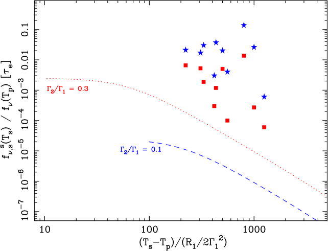
Figure 3: Similar to Figure 1 but with the GRB sample data added. The stars (squares) are our GRB sample data using the ratio between the XRT flux density at the end of the shallow X-ray decay at 1 keV and the mean BAT flux density at 100 keV (10 keV). The dashed (dotted) line is the result of our theoretical calculation.

7.2 Inverse Compton scattering in shell 2

7.2.1 Comparison between observations and theory predictions

To compare the fluxes of the X-ray shallow decay with the theoretical expectation of the inverse Compton scattering scenario, we fix the scattered frequency, $\nu_{s}$ = 1 keV. With equation (24) we can determine the frequency of the primary emission. The flux ratio data points in Figure 3 have to be changed because the frequency ratio is changed. The flux in the $\gamma$-ray band follows $f_{\nu}\propto\nu^{-\beta_{BAT}}$. With this, we can now determine that the data points in Figure 2 will be multiplied by a factor of $[\frac{\nu_{\gamma}}{\nu_{X}}(\frac{\Gamma_{2}}{\Gamma_{1}})^{2}\gamma_{e}^{2}]^{-\beta_{BAT}}$ to account for the inverse Compton scattering effect, where $\nu_{\gamma}$ and $\nu_{X}$ are the $\gamma$-ray and X-ray photon frequencies, respectively, at which the flux densities are used in the data points of Figure 3.

Since $\gamma_{e}$ is an unknown quantity we cannot determine where these new points would lie on a plot analogous to Figure 3. For this reason, we ask: what is the value of $\gamma_{e}$ necessary to lower all data points to the theoretically expected curve? To answer, let us fix the value of the Lorentz Factor ratio, $\Gamma_{2}/\Gamma_{1}=0.1$ - this is a reasonable value according to equation (22), since the $\gamma$-ray duration usually lasts $\sim 10^{2}$ s and the shallow decay extends to $\sim 10^{4}$ s.

The required values for $\gamma_{e}$ are presented in Table 2. We present two different values for each burst. We use the BAT spectral index (subscript $c$) and an average between the BAT and XRT spectral indices (subscript $e$), respectively. We do this because we are extrapolating the $\gamma$-ray flux to energies below the observed BAT band and it is unknown if the BAT spectrum will behave as a single power law in this region.

7.2.2 Electrons’ energy in shell 2

We calculate $E_{e}$ for each burst in our sample using equation (25). The results are presented in Table 2, adopting $\Gamma_{1}=10^{2}$, $\frac{\Gamma_{2}}{\Gamma_{1}}=0.1$ and $\tau_{e}$ = 0.1. Note that we have corrected $\frac{R_{1}}{2\Gamma_{1}^{2}}$ for the cosmological time dilation effect. Two values of energies from the two values of $\gamma_{e}$ obtained in the last subsection are given in the table.

Note that from equations (16) and (17) one can see that $\frac{R_{2}}{R_{1}}=\frac{1}{2}+\frac{\beta_{2}}{2\beta_{1}}-\frac{T_{s}-T_{p}}{2R_{1}}\simeq 1-\frac{1}{4\Gamma_{1}^{2}}\frac{(T_{s}-T_{p})}{R_{1}/2\Gamma_{1}^{2}}$. In our data sample $\frac{T_{s}-T_{p}}{R_{1}/2\Gamma_{1}^{2}}\leq 10^{3}$. Therefore, the approximation made in the derivation of equation (25), that $R_{2}\approx R_{1}$ for $\Gamma_{1}\sim 10^{2}$, is valid.

Table 2: Calculated values for the required $\gamma_{e}$ and total electron energy of shell 2 to obtain the theoretical expected flux ratio. The calculations were done with two different spectral indices: the BAT spectral index and the average between the BAT spectral index and the XRT spectral index.

GRB	Redshift	$\frac{R_{1}}{2\Gamma_{1}^{2}}$	$\gamma_{e}$	$E_{e}$	$\gamma_{e}$	$E_{e}$
		(s)	[$\tau_{e}^{-\frac{1}{2\beta}}$]	(erg)	[$\tau_{e}^{-\frac{1}{2\beta}}$]	(erg)
050315	1.95	10	34	5 $\times 10^{52}$	23	3 $\times 10^{52}$
050319	3.24	9.4	316	5 $\times 10^{53}$	46	5 $\times 10^{52}$
050713A		5.3	1364	1.4 $\times 10^{54}$	95	5 $\times 10^{52}$
050713B		34	2404	1.5 $\times 10^{56}$	657	3 $\times 10^{55}$
050714B		13	13	2 $\times 10^{52}$	5	7 $\times 10^{51}$
050803		24	1931	6 $\times 10^{55}$	547	1 $\times 10^{55}$
050814	5.3	23	25	2 $\times 10^{53}$	22	2 $\times 10^{53}$
050819		9.5	10	1 $\times 10^{52}$	13	1.5 $\times 10^{52}$
050822		8	21	1.6 $\times 10^{52}$	19	1.4 $\times 10^{52}$
050915B		10.5	33	6 $\times 10^{52}$	17	3 $\times 10^{52}$

7.2.3 Results

Table 2 shows that the isotropically equivalent total energy carried by the electrons of a hot shell 2 is large, $\sim 10^{52-56}$ erg. If we take into account the cooling of the electrons via adiabatic expansion and/or radiation, the initial total energy when the electrons were just accelerated is even bigger. The optical depth, $\tau_{e}$, would certainty decrease the total energy but only by a small fraction. The prompt emission from those electrons in shell 2 would arrive at about the same time as the scattered emission, and the two emission components would have similar durations because both durations are $\propto 1/\Gamma_{2}^{2}$. Depending on the ejecta properties, e.g., the ratio of the shell 2 energy to the shell 1 energy, the shell 2 prompt emission might dominate the scattered emission in the light curve. If that is true, the shell 2 prompt emission might be a possible origin of the late X-ray flares in bursts for which both the flares and the shallower decay are present.

8 Faster shell 2

In the previous section we assumed a slower shell 2. What if shell 2 is faster than shell 1? Based on the formulae we have, if $\Gamma_{2}>\Gamma_{1}$, the scattered emission from $\gamma$-rays would fall in higher energies, e.g., $\sim$ MeV, not in the X-rays, and have a shorter duration than the $\gamma$-rays.

It is shown in Figure 2 that, in the $\Gamma_{2}>\Gamma_{1}$ cases, the scattered emission is very bright though it decreases with increasing time delay. If the scattered emission spectrum mimics the power law form of the primary emission spectrum, at some time delay significantly larger than the duration of the primary emission, the lower-energy-extrapolated scattered flux is close to or even brighter than the prompt $\gamma$-rays. According to Figure 2, for $\frac{\Gamma_{2}}{\Gamma_{1}}\simeq 3$ (corresponding to $\frac{\nu_{s}}{\nu}\simeq 10$ according to equation (21)) and a selected observed time delay $(T_{s}-T_{p})/(\frac{R_{1}}{2\Gamma_{1}^{2}})\simeq 100$ (which corresponds to an ejection delay $\delta t\sim 10^{3}$s), $f_{\nu,s}^{s}(T_{s})\approx 0.1[\tau_{e}]f_{\nu}(T_{p})$. Extrapolating the scattered flux density from $\nu_{s}$ to $\nu$, we have $f_{\nu}^{s}(T_{s})=(\frac{\nu_{s}}{\nu})^{\beta_{BAT}}\times 0.1[\tau_{e}]f_{\nu}(T_{p})\approx f_{\nu}(T_{p})[\tau_{e}]$ for $\beta_{BAT}\approx$ 1. For a smaller observed time delay, the flux is even greater. That means we should have seen a lagged very short $\gamma$-ray flash at $\sim 10^{2}-10^{3}$ seconds after the burst, provided that $\tau_{e}\approx 1$. This case cannot happen because the observations have never showed this feature. Even though the flux of the scattered emission is smaller for a larger observed time delay, in order for the delayed scattered $\gamma$-ray flash to indeed happen but below the BAT flux limit, shell 2 must have an extremely large ejection time delay $\delta t\geq$ a few $\times 10^{3}$ seconds (cf. equation 17) which is very difficult to explain in terms of the central engine activity. For $\tau_{e}\ll 1$, the $\Gamma_{2}>\Gamma_{1}$ case could have happened but the flux would be too small to be detected.

One possible case of $\Gamma_{2}>\Gamma_{1}$ is that the shell 2 ejection delay $\delta t$ is small and shell 2 has moved very close to shell 1 when the scattering happens so that the observed time delay of the scattered emission is comparable or smaller than the duration of the primary emission. The scattered emission in the BAT energy range will become part of the observed prompt $\gamma$-ray emissions in time. Future high energy ($\geq$ MeV) observations (e.g., by GLAST) during the burst may be able to determine the existence of this case.

9 X-Ray dim or dark GRBs

In §7, our calculations show that the scattered flux is much lower than the observed X-ray shallow decay flux. If the scattering indeed happens, then the resultant emission must have been buried in the shallow decay. Thus, in order for the scattered emission to be detected, not only the shallow X-ray decay component must be absent, but also the normal external forward shock component must be extremely weak or absent. In rare cases Swift does observe X-ray afterglows without a shallow decay and without the normal forward shock decay ($\alpha_{X}\sim 1-1.3$), which we call X-ray dim GRBs. They show instead a very steep flux decay ($\alpha_{X}\geq 3$) and are thought to be located in extremely low density regions. The steep decay component can be explained by the large angle emission (Kumar & Panaitescu 2000). GRB 050421 and GRB 051210 are two examples (Godet et al. 2006; La Parola et al. 2006). Note that GRB 051210 is of the short burst class which, according to its compact binary progenitor model, is more probable to occur in a low density environment. At late times, however, when the large angle emission is low enough, neither burst shows any sign of re-brightening atop the steep power-law decay.

Another case of interest is the existence of X-ray dark GRBs: short bursts (GRB 050906 and GRB 050925) that show no X-ray afterglow detection, only upper limits at $\approx$ 100 s (Nakar 2007). It is also believed that these bursts took place in extremely low density environments.

X-ray dim and dark GRBs provide a great opportunity to put into work the theory presented in this paper. If we assume that there is a late ejecta behind the $\gamma$-ray producing source, then we can try to constrain its LF by looking at these bursts. Since their afterglow emission is so weak (or not present), we can ask the question: what are the constraints on the LF of the late ejecta, so that the scattered emission is present in X-ray dim and dark GRBs, but doesn’t exceed the actual flux observations or upper limits? We will devote this section to answer this question.

We’ll start by using the data from Swift’s BAT and XRT observations as follows:

$$\frac{f^{s}_{\nu,s}(T_{s})}{f_{\nu}(T_{p})}\leq\frac{f^{XRT}_{\nu,s}(T_{s})}{f^{BAT}_{\nu}(T_{90})}=0.01\frac{f^{XRT}_{1keV}(T_{s})}{f^{BAT}_{100keV}(T_{90})}\biggl{(}\frac{\Gamma_{1}}{\Gamma_{2}}\biggr{)}^{2},$$

where we have selected $\nu$ = 100 keV, but we have made no assumption on the value of $\nu_{s}$ only that it should obey equation (21). We have also assumed $\beta_{X}=1$, which is consistent with Swift observations.

With the previous inequality and using the two previously defined regions of the flux ratio (§6), we can find constraints on the LF ratio. In region I, we find:

$$\frac{\Gamma_{2}}{\Gamma_{1}}\leq\min\bigg{\{}20\biggl{(}\frac{T_{s}-T_{p}}{R_{1}/2\Gamma_{1}^{2}}\biggr{)}^{-1}\theta_{j,-1}\Gamma_{1,2},1.26f_{x\gamma}^{1/6}\tau_{e}^{-1/6}\bigg{\}}$$ (26)

and in region II:

$$20\biggl{(}\frac{T_{s}-T_{p}}{R_{1}/2\Gamma_{1}^{2}}\biggr{)}^{-1}\theta_{j,-1}\Gamma_{1,2}<\frac{\Gamma_{2}}{\Gamma_{1}}\leq$$

$$\quad\quad\quad\quad\quad 0.1f_{x\gamma}^{1/4}\biggl{(}\frac{T_{s}-T_{p}}{R_{1}/2\Gamma_{1}^{2}}\biggr{)}^{1/2}\theta_{j,-1}^{-1/2}\Gamma_{1,2}^{-1/2}\tau_{e}^{-1/4},$$ (27)

where we have used $f_{x\gamma}\equiv\frac{f^{XRT}_{1keV}(T_{s})}{f^{BAT}_{100keV}(T_{90})}$ and the convention $Q_{x}=Q/10^{x}$ has been adopted.

After presenting these last two conditions, we should return to the physical picture. The initial assumption we made is that the scattered emission should be present independently of the burst’s data and its region. This means that the LF of the late ejecta could be very small, so that its contribution to the flux would be also minuscule. Therefore, we should discard the lower limit on equation (27). Now, we want to constrain the LF of the late ejecta from above; we are interested in knowing what’s its maximum. The maximum value between the two upper limits of equations (26) and (27) will be the best and more conservative value to choose:

$$\frac{\Gamma_{2}}{\Gamma_{1}}\leq\max\left\{\begin{array}[]{ll}\min\left\{\begin{array}[]{ll}20\biggl{(}\frac{T_{s}-T_{p}}{R_{1}/2\Gamma_{1}^{2}}\biggr{)}^{-1}\theta_{j,-1}\Gamma_{1,2}\\ 1.26f_{x\gamma}^{1/6}\tau_{e}^{-1/6}\\ \end{array}\right\}\\ 0.1f_{x\gamma}^{1/4}\biggl{(}\frac{T_{s}-T_{p}}{R_{1}/2\Gamma_{1}^{2}}\biggr{)}^{1/2}\theta_{j,-1}^{-1/2}\Gamma_{1,2}^{-1/2}\tau_{e}^{-1/4}\\ \end{array}\right\}.$$

Now we are ready to consider the 4 bursts mentioned at the beginning of this section and obtain the constraints for the LF of the late ejecta.

Using the last X-ray detection of GRB 051210 (La Parola et al. 2006) and the upper limit of GRB 050421 (Godet et al. 2006), both at $\sim 10^{3}$ s, we can obtain the ratio between the XRT flux density at 1 keV (scattered emission) and the BAT flux density (Chincarini et al. 2007) at 100 keV (primary emission), $f_{x\gamma}$. Following the procedure outlined in §7.1.1, the values for $\frac{T_{s}-T_{p}}{R_{1}/2\Gamma_{1}^{2}}$ are also obtained. We can do exactly the same for the X-ray dark short GRBs, using the upper limits of GRB 050906 and GRB 050925 at $\approx$ 100 s (Pagani et al. 2005; Beardmore et al. 2005; Nakar 2007). With $f_{x\gamma}$ and the normalized time delay, we find the following constraints:

$$\frac{\Gamma_{2}}{\Gamma_{1}}(\theta_{j,-1}\Gamma_{1,2})^{1/2}\tau_{e}^{1/4}\lower 2.0pt\hbox{$\,\buildrel\scriptstyle<\over{\scriptstyle\sim}\,$}\left\{\begin{array}[]{ll}0.15&\textrm{for GRB 050906 and 050925,}\\ 0.48&\textrm{for GRB 050421,}\\ 0.78&\textrm{for GRB 051210.}\\ \end{array}\right.$$

The upper limits for the X-ray dark short GRBs provide the best constraints, since the upper limits in their X-ray flux are very strict. These results imply that, for $\tau_{e}=1$, $\Gamma_{1}=100$ and $\theta_{j}=0.1$, the late ejecta is very slow $\Gamma_{2}\lower 2.0pt\hbox{$\,\buildrel\scriptstyle<\over{\scriptstyle\sim}\,$}15$, but it could be faster if $\tau_{e}$ decreases.

10 Summary and Conclusions

We have investigated a scenario of photons scattering by electrons within a relativistic outflow. The outflow is composed of discrete shells. One front shell emits radiation, observed as the GRB’s prompt $\gamma$-ray photons. Some fraction of the radiation is incident backwards to the shell(s) behind, and is scattered isotropically in the local rest frame. The scattered emission arrives at the observer at a later time, $T_{s}$, and at a different photon energy, $\nu_{s}$, that are determined by the LF ratio of the two shells and the time delay of the ejection of the second shell. We calculated the flux density ratio, i. e., the flux density of the delayed scattered emission to that of the front shell’s primary emission, as a function of the normalized arrival time delay and the assumed LF ratio.

The calculated flux density ratio are compared with observations using a sample of Swift GRB X-ray afterglows which show a distinct shallower decay component in their light curves, with the motivation to see if the scattering scenario could be the origin of the shallower decay. The results are negative. For Thomson scattering, the flux density of the scattered emission is about $10^{3-4}\tau_{e}^{-1}$ times lower than that of the shallower decay component, where $\tau_{e}$ is the scattering shell’s electron optical depth.

We also consider the inverse Compton scattering scenario in which the electrons in the scattering shell is hot. We find that, in order for the scattered emission flux to be bright enough to match the shallower decay component, the isotropic equivalent of the total energy carried by the hot electrons is large, $\sim 10^{52-56}$ erg. The prompt emission from the scattering shell appears at the same time as the scattered emission and with a similar duration.

In the cases where shell 2 is faster than shell 1, when extrapolated to the BAT energy band, the scattered flux can be as bright as the emission from shell 1. The delay of the scattered emission is determined by the ejection delay of shell 2. When the ejection delay of shell 2 is much larger than the duration of the primary emission, the scattered emission would appear as a late short $\gamma$-ray/MeV flash. For a small ejection delay of shell 2, the scattered emission would become part of the observed prompt emission. The fact that no late short $\gamma$-ray/MeV flash is detected does not support the existence of a late faster shell.

Lastly, we study the possibility of detection of the scattering emission in two X-ray dim GRBs - that only show a very steep flux decay and do not show either a X-ray shallow decay nor the normal forward shock component - and in two X-ray dark short GRBs - that show no X-ray afterglow detection at $\sim$ 100 s. Assuming that there is slower moving ejecta material behind the fast $\gamma$-ray producing shell in these bursts, we find upper limits for the Lorentz factor of the late slower material. More sensitive observations of X-ray dark short GRBs could provide stronger constraints on the presence and properties of slower moving material accompanying the fast $\gamma$-ray jet in GRBs.

Almost simultaneous to the appearance of this paper, Panaitescu (2007) presents a similar work on the scattering of the GRB early emission photons by a late outflow. Both papers present the same physics and the main formulae are consistent. The main differences are that (i) we have considered the scattering within the relativistic outflow and the photons to be scattered are the prompt $\gamma$-ray photons, whereas Panaitescu (2007) considers the scattering of the afterglow forward shock photons by a late relativistic outflow, and (ii) Panaitescu (2007) has considered a faster second shell to be able to explain features like the “shallow decay” and the X-ray flares, whereas our focus is mostly on a slower second shell.

APPENDIX: Approximation to the integrand function in calculation of the incident flux on shell 2

Here we show that the integrand function in equation (6) for the incident flux from shell 1 on point $P$ in shell 2 comoving frame is insensitive to $\sin^{2}\alpha^{\prime\prime}$ so that the integrand can be taken out of the integral as a constant. We will also show that the integrand is of order unity.

Let us call the integrand function $F(\alpha,\theta)$. All equations we have are

$$F(\alpha,\theta)=\frac{(1+\beta_{2}\cos\alpha)^{3}}{[\beta_{1}+\cos(\alpha-\theta)][1+\beta_{1}\cos(\alpha-\theta)]^{2}}$$ (A-1)

$$\tan\alpha^{\prime\prime}=\frac{\theta}{\Gamma_{2}(1-\frac{\beta_{2}}{\beta_{1}}+\frac{\beta_{2}\delta t}{R_{1}})}$$ (A-2)

$$\tan\alpha^{\prime\prime}=\frac{\sin\alpha}{\Gamma_{2}(\cos\alpha+\beta_{2})}.$$ (A-3)

We want to precisely estimate $F(\alpha,\theta)$ and its dependence on $\sin^{2}\alpha^{\prime\prime}$ in the range of $\alpha^{\prime\prime}$ from 0 to $\alpha_{j}^{\prime\prime}$, where the subscript “j” always denotes the edge of shell 1. Through equations (A-2) and (A-3), we can express $\theta$ in terms of $\alpha$ only:

$$\theta=\frac{\sin\alpha(1-\frac{\beta_{2}}{\beta_{1}}+\frac{\beta_{2}\delta t}{R_{1}})}{\cos\alpha+\beta_{2}}.$$ (A-4)

Then $F(\alpha,\theta)$ becomes $F(\alpha)$. Also, from equation (A-3), express $\sin^{2}\alpha^{\prime\prime}$ in terms of $\alpha$ only:

$$\sin^{2}\alpha^{\prime\prime}=\frac{\sin^{2}\alpha}{\sin^{2}\alpha+\Gamma_{2}^{2}(\cos\alpha+\beta_{2})}.$$ (A-5)

Therefore, we can plot $F(\alpha)$ numerically as a function of $\sin^{2}\alpha^{\prime\prime}$.

The only thing left is to calculate the upper limit of $\alpha$. Equation (A-2) gives

$$\tan\alpha_{j}^{\prime\prime}=\frac{\theta_{j}}{\Gamma_{2}(1-\frac{\beta_{2}}{\beta_{1}}+\frac{\beta_{2}\delta t}{R_{1}})}.$$ (A-6)

Denote $k=\tan\alpha_{j}^{\prime\prime}$, and apply it onto equation (A-3) and square both sides of (A-3). Then we get a quadratic equation of $\cos\alpha_{j}$:

$$(1+k^{2}\Gamma_{2}^{2})\cos^{2}\alpha_{j}+2\beta_{2}k^{2}\Gamma_{2}^{2}\cos\alpha_{j}+k^{2}\Gamma_{2}^{2}\beta_{2}^{2}-1=0,$$ (A-7)

with roots

$$\cos\alpha_{j}=\frac{-\beta_{2}k^{2}\Gamma_{2}^{2}\pm\sqrt{k^{2}+1}}{1+k^{2}\Gamma_{2}^{2}}.$$ (A-8)

The second root ($-$) can be ruled out, because when we put it back into equation (A-3), the second root gives $k<0$, while equation (A-2) requires $k>0$. Thus

$$\alpha_{j}=\arccos\biggl{(}\frac{-\beta_{2}\Gamma_{2}^{2}k^{2}+\sqrt{k^{2}+1}}{1+k^{2}\Gamma_{2}^{2}}\biggr{)}$$ (A-9)

is the sole root of the upper limit of $\alpha$.

We numerically plot $F(\alpha)$ vs. $\sin^{2}\alpha^{\prime\prime}$ for the following model parameter space: $\frac{\Gamma_{2}}{\Gamma_{1}}$ ranges from 0.05 to 10, $\frac{\delta t}{R_{1}/(2\Gamma_{1}^{2})}$ ranges from 0 to 1000, and $\theta_{j}$= 0.1. We find, for $\frac{\Gamma_{2}}{\Gamma_{1}}<1$, $F(\alpha)$ is approximately a linear, monotonically decreasing function of $\sin^{2}\alpha^{\prime\prime}$. Its maximum is 1 and is at $\alpha=0$, and minimum is always $>$ 0.01 and is at $\alpha=\alpha_{j}$. A smaller $\frac{\Gamma_{2}}{\Gamma_{1}}$ or a larger $\delta t$ always gives a smaller $\alpha_{j}$, thus a minimum of $F(\alpha)$ closer to 1.

This clearly shows that for $\frac{\Gamma_{2}}{\Gamma_{1}}<1$, $F(\alpha)$ is very weakly dependent on $\sin^{2}\alpha^{\prime\prime}$ thus can be taken out of the integral as a constant $\sim$ 1.

For $\frac{\Gamma_{2}}{\Gamma_{1}}>1$, $F(\alpha)$ is not always on order of unity. Since shell 2 is moving toward shell 1, the relativistic beaming effect is important (Panaitescu 2007). When $\delta t$ is very small, shell 2 is very close to shell 1, so that $\alpha_{j}^{\prime\prime}$ is larger than $\frac{1}{\Gamma_{rel}}$, where $\Gamma_{rel}\simeq\frac{\Gamma_{2}}{2\Gamma_{1}}$ is the relative LF between two shells. In this case we find that at an angle $\alpha^{\prime\prime}<\alpha_{j}^{\prime\prime}$, $F(\alpha)$ starts to drop very sharply from on order of unity to infinitely small, and that dropping-down angle is approximately equal to $\frac{1}{\Gamma_{rel}}$. This means that, in the case of $\frac{\Gamma_{2}}{\Gamma_{1}}>1$, $\sin^{2}{\alpha_{j}^{\prime\prime}}$ in equation (14) should be replaced by a more accurate term $\min(\sin^{2}{\alpha_{j}^{\prime\prime}},\frac{1}{\Gamma_{rel}^{2}})$. However this is only required when $\delta t$ is small so that $\frac{T_{s}-T_{p}}{R_{1}/(2\Gamma_{1}^{2})}<100$. Thus the more accurate flux ratio curves for $\frac{\Gamma_{2}}{\Gamma_{1}}>1$ in our Figure 2 will be slightly flatter in the region of $\frac{T_{s}-T_{p}}{R_{1}/(2\Gamma_{1}^{2})}<100$ than the ones shown. But our conclusion about a faster shell 2 is not affected.

References

- [1] Beardmore A. P., Page K. L., Gehrels N., Greiner J., Kennea J., Nousek J., Osborne J. P., Tagliaferri G., 2005, GCN Circ., 4043
- [2] Chincarini G. et al., 2007, ApJ, 671, 1903
- [3] Esin A. A., Blandford R., 2000, ApJ, 534, L151
- [4] Fynbo J. P. U., Hjorth J., Jensen B., Jakobsson P., Moller P., Näränen J., 2005, GCN Circ., 3136
- [5] Godet O. et al., 2006, A&A, 452, 819
- [6] Heng K., Lazzati D., Perna R., 2007, ApJ, 662, 1119
- [7] Jakobsson P. et al., 2006, A&A, 447, 897
- [8] Kelson D., Berger E., 2005, GCN Circ., 3101
- [9] Kumar P., Panaitescu A. 2000, ApJ, 541, L51
- [10] La Parola V. et al., 2006, A&A, 454, 753
- [11] Madau P., Blandford R. D., Rees M. J., 2000, ApJ, 541, 712
- [12] Nakar E., 2007, Phys. Rep., 442, 166
- [13] Nousek J. A. et al., 2006, ApJ, 642, 389
- [14] O’Brien P. et al., 2006, ApJ, 647, 1213
- [15] Pagani C., La Parola V., Burrows D. N., 2005, GCN Circ., 3934
- [16] Panaitescu A., 2007, MNRAS, in press, preprint (arxiv:0708.1509)
- [17] Piran T., 2005, Rev. Mod. Phys., 76, 1143
- [18] Rybicki G. B., Lightman A. P., 1979, Radiative Processes in Astrophysics. Wiley-Interscience Press, New York.
- [19] Shao L., Dai Z. G., 2007, ApJ, 660, 1319
- [20] Zhang B., 2007, Chin. J. Astron. Astrophys. 7, 1