Entangling a nanomechanical resonator and a superconducting microwave cavity

Abstract

We propose a scheme able to entangle at the steady state a nanomechanical resonator with a microwave cavity mode of a driven superconducting coplanar waveguide. The nanomechanical resonator is capacitively coupled with the central conductor of the waveguide and stationary entanglement is achievable up to temperatures of tens of milliKelvin.

I Introduction

Entanglement is one of a number of inherently quantum phenomena that it is hoped will soon be observable in macroscopic mechanical systems Blencowe1 . Aside from the interest in studying quantum mechanics in a new regime, entanglement may be used as part of read-out schemes in quantum information processing applications. Methods for entangling a nanomechanical resonator with a Cooper pair box armour1 , or an optical mode Vitali07 , for entangling two charge qubits zou1 or two Josephson junctions cleland1 via nanomechanical resonators, and for entangling two nanomechanical resonators via trapped ions tian1 , Cooper pair boxes tian2 , entanglement swapping Pir06 , and sudden switching of electrical interactions plenio1 , have all been proposed. In the earliest proposal, armour1 , the entanglement provided a means for measuring the decoherence rate of coherent superpositions of nanomechanical resonator states. More recently, a scheme for entangling a superconducting coplanar waveguide field with a nanomechanical resonator, via a Cooper pair box within the waveguide ringsmuth , was proposed.

Here we propose a different scheme for entangling the nanomechanical resonator, based on the capacitive coupling of the resonator with the central conductor of the superconducting, coplanar waveguide, and which does not require any Cooper pair box (see Ref. tian3 for a related proposal). The paper is organized as follows. In Sec. II we derive the Quantum Langevin equations (QLE) of the system and discuss when they can be linearized around the semiclassical steady state. In Section III we study the steady state of the system and quantify its entanglement by using the logarithmic negativity, while Section IV is for conclusions.

II Quantum Langevin equations and their linearization

The proposed scheme is shown in Figure 1: a nanomechanical resonator is capacitively coupled to the central conductor of a superconducting, coplanar waveguide that forms a microwave cavity of resonant frequency $\omega_{c}$. The cavity is driven at a frequency $\omega_{0}=\omega_{c}-\Delta_{0}$. In view of the equivalent circuit, the effective Hamiltonian for the coupled system is

$$H=\frac{p_{x}^{2}}{2m}+\frac{m\omega_{m}^{2}x^{2}}{2}+\frac{\Phi^{2}}{2L}+\frac{Q^{2}}{2(C+C_{0}(x))}-e(t)Q,$$ (1)

where $(x,p_{x})$ are the canonical position and momentum of the resonator, and $(\Phi,Q)$ are the canonical coordinates for the cavity, representing respectively the flux through an equivalent inductor $L$ and the charge on an equivalent capacitor $C$.

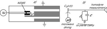
Figure 1: Schematic representation of the capacitive coupling between a nanomechanical resonator and a superconducting coplanar microwave cavity. (a) Plan view of the device; the dark region is etched away and the resulting cantilever is metalized to form one plate of a capacitor. (b) Equivalent circuit.

The coherent driving of the cavity is given by the electric potential $e(t)=-i\sqrt{2\hbar\omega_{c}L}E(e^{i\omega_{0}t}-e^{-i\omega_{0}t})$. The function $C_{0}(x)$ describes the capacitive coupling between the cavity and the resonator, as a function of the resonator displacement $x$. Expanding this around the equilibrium position of the resonator at $d$ from the cavity and with capacitance $C_{0}$, we have $C_{0}(x)=C_{0}(1-x(t)/d)$. Expanding the capacitive energy as a Taylor series, we find to first order,

$$\frac{Q^{2}}{2(C+C_{0}(x))}=\frac{Q^{2}}{2C_{\Sigma}}+\frac{\beta}{2dC_{\Sigma}}x(t)Q^{2},$$ (2)

where $C_{\Sigma}=C+C_{0}$ and $\beta=C_{0}/C_{\Sigma}$.

We can now quantize the Hamiltonian, promoting the canonical coordinates to operators with $[\hat{x},\hat{p}_{x}]=[\hat{Q},\hat{\Phi}]=i\hbar$. The quantum Hamiltonian, in terms of the raising and lowering operators for the cavity ($a^{\dagger},a$) and the resonator dimensionless canonical operators $(\hat{q},\hat{p})$, is

$$H = \hbar\omega_{c}a^{\dagger}a+\frac{\hbar\omega_{m}}{2}(\hat{q}^{2}+\hat{p}^{2})+\hbar\frac{G_{0}}{2}\hat{q}(a+a^{\dagger})^{2}$$ (3)

$$\ \ -i\hbar E(e^{i\omega_{0}t}-e^{-i\omega_{0}t})(a+a^{\dagger}),$$

where

$$a = \sqrt{\frac{\omega_{c}L}{2\hbar}}\hat{Q}+\frac{i}{\sqrt{2\hbar\omega_{c}L}}\hat{\Phi},$$ (4)

$$\hat{q} = \sqrt{\frac{m\omega_{m}}{\hbar}}\hat{x},\;\;\hat{p}=\frac{\hat{p}_{x}}{\sqrt{\hbar m\omega_{m}}},$$ (5)

and the coupling depends on

$$G_{0}=\beta\omega_{c}\left(\frac{1}{2d}\sqrt{\frac{\hbar}{m\omega_{m}}}\right).$$ (6)

Typically, $\omega_{c}\gg\omega_{m}$ since $\omega_{c}/2\pi\approx 10$ GHz schoelkopf , while $\omega_{m}/2\pi\approx 20$ MHz schwab . It is convenient to move into an interaction picture with respect to $\hbar\omega_{0}a^{\dagger}a$, and neglect terms oscillating at $\pm 2\omega_{0}$. The resulting Hamiltonian is

$$H_{I}=\hbar\Delta_{0}a^{\dagger}a+\frac{\hbar\omega_{m}}{2}(\hat{q}^{2}+\hat{p}^{2})+\hbar G_{0}\hat{q}a^{\dagger}a-i\hbar E(a-a^{\dagger}).$$ (7)

The coupling term represents a low frequency modulation of the cavity resonance frequency. This will cause a phase modulation of the cavity field and write sidebands onto the cavity spectrum at multiples of $\omega_{m}$ from $\omega_{c}$.

The resonator has a mechanical damping rate $\gamma_{m}$ and the cavity bandwidth is $2\kappa$. System dynamics also depend on the cavity input noise $a^{in}(t)$, where

$$\langle a^{in,{\dagger}}(t)a^{in}(t^{\prime})\rangle=\bar{n}_{a}\delta(t-t^{\prime}),$$ (8)

with $\bar{n}_{a}=\left(\exp\{\hbar\omega_{c}/k_{B}T\}-1\right)^{-1}$, and also on the Brownian noise acting on the cavity ends $\xi(t)$, with correlation function GIOV01

$$\left\langle\xi(t)\xi(t^{\prime})\right\rangle=\frac{\gamma_{m}}{\omega_{m}}\int\frac{d\omega}{2\pi}e^{-i\omega(t-t^{\prime})}\omega\left[\coth\left(\frac{\hbar\omega}{2k_{B}T}\right)+1\right].$$ (9)

Clearly, $\xi(t)$ is not delta-correlated and does not describe a Markovian process. However, quantum effects are achievable only when using resonators with a large mechanical quality factor $(\mathcal{Q}_{m}=\omega_{m}/\gamma_{m}\gg 1)$, and in this limit $\xi(t)$ becomes delta-correlated benguria ,

$$\left\langle\xi(t)\xi(t^{\prime})+\xi(t^{\prime})\xi(t)\right\rangle/2\simeq\gamma_{m}\left(2\bar{n}_{b}+1\right)\delta(t-t^{\prime}),$$ (10)

where $\bar{n}_{b}=\left(\exp\{\hbar\omega_{m}/k_{B}T\}-1\right)^{-1}$, and we recover a Markovian process. Adding these inputs to the equations of motion that follow from (7), we obtain the nonlinear quantum Langevin equations (QLEs)

$$\dot{q} = \omega_{m}p,$$ (11a)

$$\dot{p} = -\omega_{m}q-\gamma_{m}p+G_{0}a^{{\dagger}}a+\xi,$$ (11b)

$$\dot{a} = -(\kappa+i\Delta_{0})a+iG_{0}aq+E+\sqrt{2\kappa}a^{in}.$$ (11c)

Neglecting the noise and treating the deterministic equations as classical, with $a\rightarrow\alpha$ a complex field amplitude, we find the fixed points of the system by setting the left hand side of Eqs.(11) to zero. The fixed points are then given by

$$p_{s} = 0,$$ (12)

$$q_{s} = \frac{G_{0}}{\omega_{m}}n_{s},$$ (13)

$$E^{2} = n_{s}\left(\kappa^{2}+(\Delta_{0}-G_{0}^{2}n_{s}/\omega_{m})^{2}\right),$$ (14)

where the steady state photon number in the cavity is defined as $n_{s}=|\alpha_{s}|^{2}$. Eq. (14) is the same as the equation of state for optical bistability in a dispersive non linear medium WallsMilb and thus we expect for $\Delta_{0}>0$ there will be multiple stable fixed points.

The quantum dynamics of the full nonlinear system is difficult to analyze so we linearize around the semiclassical fixed points. That is, we write $a=\alpha_{s}+\delta a$, $q=q_{s}+\delta q$ and $p=p_{s}+\delta p$. This decouples our system into a set of nonlinear algebraic equations for the steady-state values and a set of QLEs for the fluctuation operators. The steady-state values are given by Eqs. (12) and (13), and $\alpha_{s}=E/(\kappa+i\Delta)$; an implicit equation for $\alpha_{s}$, since the effective detuning $\Delta$ is given by $\Delta=\Delta_{0}-G_{0}^{2}|\alpha_{s}|^{2}/\omega_{m}$. The QLEs for the fluctuations are

$$\delta\dot{q} = \omega_{m}\delta p,$$ (15a)

$$\delta\dot{p} = -\omega_{m}\delta q-\gamma_{m}\delta p+G_{0}\left(\alpha_{s}\delta a^{{\dagger}}+\alpha_{s}^{*}\delta a\right)$$ (15b)

$$+\delta a^{{\dagger}}\delta a+\xi,$$

$$\delta\dot{a} = -(\kappa+i\Delta)\delta a+iG_{0}\left(\alpha_{s}+\delta a\right)\delta q+\sqrt{2\kappa}a^{in}.$$ (15c)

Provided the cavity is driven intensely, $|\alpha_{s}|\gg 1$, we can safely neglect the terms $\delta a^{{\dagger}}\delta a$ in Eq. (15b) and $\delta a\delta q$ in Eq. (15c), and obtain the linearized QLEs

$$\delta\dot{q} = \omega_{m}\delta p,$$ (16a)

$$\delta\dot{p} = -\omega_{m}\delta q-\gamma_{m}\delta p+G_{0}\alpha_{s}\left(\delta a^{{\dagger}}+\delta a\right)+\xi,$$ (16b)

$$\delta\dot{a} = -(\kappa+i\Delta)\delta a+iG_{0}\alpha_{s}\delta q+\sqrt{2\kappa}a^{in},$$ (16c)

where we have chosen the phase reference so that $\alpha_{s}$ can be taken as real.

III Steady state of the system and its entanglement properties

In order to characterize the steady state of the system, it is convenient to rewrite Eqs. (16), defining $G=G_{0}\alpha_{s}\sqrt{2}$, in terms of the field quadratures $\delta X=(\delta a+\delta a^{\dagger})/\sqrt{2}$ and $\delta Y=-i(\delta a-\delta a^{\dagger})/\sqrt{2}$, that is,

$$\delta\dot{q} = \omega_{m}\delta p,$$ (17a)

$$\delta\dot{p} = -\omega_{m}\delta q-\gamma_{m}\delta p+G\delta X+\xi,$$ (17b)

$$\delta\dot{X} = -\kappa\delta X+\Delta\delta Y+\sqrt{2\kappa}X^{in},$$ (17c)

$$\delta\dot{Y} = -\kappa\delta Y-\Delta\delta X+G\delta q+\sqrt{2\kappa}Y^{in},$$ (17d)

where $X^{in}=(\delta a^{in}+\delta a^{in,\dagger})/\sqrt{2}$ and $Y^{in}=-i(\delta a^{in}-\delta a^{in,\dagger})/\sqrt{2}$. In matrix form, Eqs. (17) can be written as

$$\dot{u}(t)=Au(t)+n(t),$$ (18)

where $u^{T}(t)=(\delta q(t),\delta p(t),\delta X(t),\delta Y(t))$, $n^{T}(t)=(0,\xi(t),\sqrt{2\kappa}X^{in}(t),\sqrt{2\kappa}Y^{in}(t))$ and

$$A=\left(\begin{array}[]{cccc}0&\omega_{m}&0&0\\ -\omega_{m}&-\gamma_{m}&G&0\\ 0&0&-\kappa&\Delta\\ G&0&-\Delta&-\kappa\end{array}\right),$$ (19)

Eq. (18) has the solution

$$u(t)=M(t)u(0)+\int_{0}^{t}dsM(s)n(s),$$ (20)

where $M(t)=\exp(At)$. The stability conditions can be derived by applying the Routh-Hurwitz criterion grad ,

$$s_{1} = 2\gamma_{m}\kappa\left\{\left[\kappa^{2}+\left(\omega_{m}-\Delta\right)^{2}\right]\left[\kappa^{2}+\left(\omega_{m}+\Delta\right)^{2}\right]\right.$$ (21a)

$$\left.+\gamma_{m}\left[\left(\gamma_{m}+2\kappa\right)\left(\kappa^{2}+\Delta^{2}\right)+2\kappa\omega_{m}^{2}\right]\right\}$$

$$+\Delta\omega_{m}G^{2}\left(\gamma_{m}+2\kappa\right)^{2}>0,$$

$$s_{2} = \omega_{m}\left(\Delta^{2}+\kappa^{2}\right)-G^{2}\Delta>0.$$ (21b)

For driving on the blue sideband of the cavity $(\Delta=-\omega_{m})$ we have

$$G < \left\{2\gamma_{m}\kappa\left(\kappa^{4}+4\omega^{2}_{m}\kappa^{2}+\gamma^{2}_{m}\kappa^{2}+4\gamma_{m}\kappa\omega^{2}_{m}\right.\right.$$ (22)

$$\left.\left.\ \ +2\gamma_{m}\kappa^{3}+\gamma^{2}_{m}\omega^{2}_{m}\right)\right\}^{\frac{1}{2}}/\left\{\omega_{m}(\gamma_{m}+2\kappa)\right\},$$

while for driving on the red sideband $(\Delta=\omega_{m})$,

$$G<\sqrt{\omega^{2}_{m}+\kappa^{2}}.$$ (23)

Since the noise terms in Eq. (18) are zero-mean Gaussian and the dynamics are linear, the steady-state for the fluctuations is a two-mode Gaussian state, fully characterized by its symmetrically-ordered $4\times 4$ correlation matrix. This has components $V_{ij}=\langle u_{i}(\infty)u_{j}(\infty)+u_{j}(\infty)u_{i}(\infty)\rangle/2$. When the system is stable, using (20), we get

$$V_{ij}=\sum_{k,l}\int_{0}^{\infty}ds\int_{0}^{\infty}ds^{\prime}M(s)_{ik}M(s^{\prime})_{jl}\Phi(s-s^{\prime})_{kl},$$ (24)

where $\Phi(s-s^{\prime})_{kl}=\langle n(s)_{k}n(s^{\prime})_{l}+n(s^{\prime})_{l}n(s)_{k}\rangle/2$ is the matrix of stationary noise correlation functions. Here $\Phi(s-s^{\prime})_{kl}=D_{kl}\delta(s-s^{\prime})$, where $D=\mathrm{Diag}[0,\gamma_{m}(2\bar{n}_{b}+1),2\kappa(\bar{n}_{a}+1/2),2\kappa(\bar{n}_{a}+1/2)]$ and (24) becomes

$$V=\int_{0}^{\infty}dsM(s)DM(s)^{T}$$ (25)

which, by Lyapunov’s first theorem parks , is equivalent to

$$AV+VA^{T}=-D.$$ (26)

Solving this equation, we can then quantify the entanglement of the steady-state by means of the logarithmic negativity, $E_{\mathcal{N}}$ werner ; Salerno1 . This entanglement measure is particularly convenient because it is the only one which can always be explicitly computed and it is also additive supernote . In the continuous variable case we have

$$E_{\mathcal{N}}=\max[0,-\ln 2\eta]$$ (27)

where $\eta=2^{-1/2}\left[\Sigma(V)-\left[\Sigma(V)^{2}-4\det V\right]^{1/2}\right]^{1/2}$, with $\Sigma(V)$ expressed in terms of the $2\times 2$ block matrix

$$V=\left[\begin{array}[]{cc}V_{b}&V_{corr}\\ V_{corr}^{T}&V_{a}\end{array}\right]$$ (28)

as $\Sigma(V)=\det V_{b}+\det V_{a}-2\det V_{corr}$.

The logarithmic negativity, assuming $\Delta=\pm\omega_{m}$, depends on $T$, $G$, $\omega_{c}$, $\kappa$, $\omega_{m}$ and $\gamma_{m}$. We first consider the zero-temperature entanglement, such that our results are independent of $T$ and $\omega_{c}$. In all cases, entanglement increases with increasing coupling $G$; the limit on our entanglement being due to the limit on $G$ specified by our stability conditions, (22) and (23), and we shall set $G$ just below this threshold. At zero temperature, the absolute magnitude of $\omega_{m}$ is also insignificant, so we may hold it fixed (at $\omega_{m}=5\times 10^{8}s^{-1}$, say), leaving $\kappa$ and $\gamma_{m}$ as our remaining free parameters. It is implicitly assumed here that damping rates are controllable independent of resonant frequencies. The zero-temperature $E_{\mathcal{N}}$ is shown in Figures 2(a) and 2(b) for driving on the blue and red sidebands, respectively. From this data, along with the stability conditions, we note that on the blue sideband, entanglement is maximized in a regime where $\omega_{m}\gg G,\kappa$. This is not the case for driving on the red sideband. We also observe that the logarithmic negativity plateaus in both cases as $\kappa$ and $\gamma_{m}$ increase.

Now the temperature dependence of the entanglement follows from the Planck distributions specifying the noise input correlation functions, Eqs. (37) and (10); hence the magnitudes of the resonant frequencies become significant in these calculations. Typical temperature dependence of the logarithmic negativity is shown in Figure 3(a), decreasing from a positive value at zero temperature to zero at a temperature we shall refer to as the critical temperature, $T_{c}$. Now $T_{c}$ increases both with increasing $\omega_{c}$ and $\omega_{m}$; henceforth, we shall consider these fixed, with $\omega_{c}=10^{10}s^{-1}$. The dependence of $T_{c}$ on the damping is shown in Figures 3(b) and 3(c); the entanglement in the red sideband case appears more robust with respect to increases in temperature.

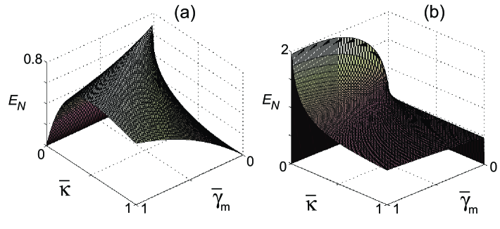
Figure 2: Zero-temperature logarithmic negativity for (a) driving on the blue sideband, (b) driving on the red sideband. $\bar{\kappa}=\kappa\times 10^{-6}{\rm s}^{-1}$, $\bar{\gamma}_{m}=\gamma_{m}\times 10^{-6}{\rm s}^{-1}$

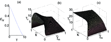
Figure 3: (a) Typical temperature, $T$ (mK) dependence of the logarithmic negativity (in this case, driving on the blue sideband with $\kappa=\gamma_{m}=5\times 10^{4}s^{-1}$). (b) $T_{c}$ (mK) as a function of damping for driving on the blue sideband. (c) $T_{c}$ (mK)as a function of damping for driving on the red sideband. $\bar{\kappa}=\kappa\times 10^{-6}{\rm s}^{-1}$, $\bar{\gamma}_{m}=\gamma_{m}\times 10^{-6}{\rm s}^{-1}$

III.1 Results in the rotating wave approximation

The results in the regime $\omega_{m}\gg G,\kappa$ may be understood with the aid of a rotating wave approximation (RWA) calculation. We will refer to this as weak driving as $G$ depends on $n_{s}$, the intracavity photon number, which itself depends on the strength of the driving field, $E$. It is then useful to introduce the nanomechanical annihilation operator $\delta b=(\delta q+i\delta p)/\sqrt{2}$, such that Eqs. (16a) and (16b) are equivalent to

$$\delta\dot{b}=-i\omega_{m}\delta b-\frac{\gamma_{m}}{2}\left(\delta b-\delta b^{\dagger}\right)+i\frac{G}{2}\left(\delta a^{{\dagger}}+\delta a\right)+\frac{\xi}{\sqrt{2}}$$ (29)

and the whole system is described in terms of annihilation and creation fluctuation operators by Eqs. (16c) and (29). We now move to a further interaction picture by introducing the slowly-moving tilded operators $\delta b(t)=\delta\tilde{b}(t)e^{-i\omega_{m}t}$ and $\delta a(t)=\delta\tilde{a}(t)e^{-i\Delta t}$. They obey the QLEs

$$\delta\dot{\tilde{b}} = -\frac{\gamma_{m}}{2}\left(\delta\tilde{b}-\delta\tilde{b}^{\dagger}e^{2i\omega_{m}t}\right)+\frac{\xi e^{i\omega_{m}t}}{\sqrt{2}},$$ (30)

$$\ \ +i\frac{G}{2}\left(\delta\tilde{a}^{{\dagger}}e^{i(\Delta+\omega_{m})t}+\delta\tilde{a}e^{i(\omega_{m}-\Delta)t}\right)$$

$$\delta\dot{\tilde{a}} = -\kappa\delta\tilde{a}+i\frac{G}{2}\left(\delta\tilde{b}^{{\dagger}}e^{i(\Delta+\omega_{m})t}+\delta\tilde{b}e^{i(\Delta-\omega_{m})t}\right)$$ (31)

$$\ \ +\sqrt{2\kappa}a^{in}e^{i\Delta t}.$$

The RWA allows us to ignore terms rotating at $\pm 2\omega_{m}$ and use $\Delta\approx\Delta_{0}$. Then, for driving on the blue sideband we have $\omega_{c}\simeq\omega_{0}-\omega_{m}$ and

$$\delta\dot{\tilde{b}} = -\frac{\gamma_{m}}{2}\delta\tilde{b}+i\frac{G}{2}\delta\tilde{a}^{{\dagger}}+\sqrt{\gamma_{m}}b^{in},$$ (32)

$$\delta\dot{\tilde{a}} = -\kappa\delta\tilde{a}+i\frac{G}{2}\delta\tilde{b}^{{\dagger}}+\sqrt{2\kappa}\tilde{a}^{in},$$ (33)

and for driving on the red sideband we have $\omega_{c}\simeq\omega_{0}+\omega_{m}$ and

$$\delta\dot{\tilde{b}} = -\frac{\gamma_{m}}{2}\delta\tilde{b}+i\frac{G}{2}\delta\tilde{a}+\sqrt{\gamma_{m}}b^{in},$$ (34)

$$\delta\dot{\tilde{a}} = -\kappa\delta\tilde{a}+i\frac{G}{2}\delta\tilde{b}+\sqrt{2\kappa}\tilde{a}^{in}.$$ (35)

Note that $\tilde{a}^{in}(t)=a^{in}(t)e^{i\Delta t}$, possessing the same correlation function as $a^{in}(t)$, and $b^{in}(t)=\xi(t)e^{i\omega_{m}t}/\sqrt{2}$ which, in the limit of large $\omega_{m}$, acquires the correlation functions gard

$$\langle b^{in,{\dagger}}(t)b^{in}(t^{\prime})\rangle = \bar{n}_{b}\delta(t-t^{\prime}),$$ (36)

$$\langle b^{in}(t)b^{in,{\dagger}}(t^{\prime})\rangle = \left[\bar{n}_{b}+1\right]\delta(t-t^{\prime}).$$ (37)

From Eqs. (32)-(33) we see that, for driving on the blue sideband, the cavity mode and nanomechanical mode play the role of the signal and the idler of a nondegenerate parametric oscillator, characterized by an interaction term $\delta\tilde{b}^{{\dagger}}\delta\tilde{a}^{{\dagger}}+\delta\tilde{a}\delta\tilde{b}$. Therefore, it can generate entanglement. However, from Eqs. (34)-(35), in the red sideband case the two modes are coupled by the beamsplitter-like interaction $\delta\tilde{b}^{\dagger}\delta\tilde{a}+\delta\tilde{a}^{\dagger}\delta\tilde{b}$, which is not able to entangle modes starting from classical input states kim .

Now introduce tilded quadrature operators $\delta\tilde{X}=(\delta\tilde{a}+\delta\tilde{a}^{{\dagger}})/\sqrt{2}$ and $\delta\tilde{Y}=(\delta\tilde{a}-\delta\tilde{a}^{{\dagger}})/i\sqrt{2}$, with corresponding input noise operators $X^{in}=(\tilde{a}^{in}+\tilde{a}^{in,{\dagger}})/\sqrt{2}$, $Y^{in}=(\tilde{a}^{in}-\tilde{a}^{in,{\dagger}})/i\sqrt{2}$, $q^{in}=(b^{in}+b^{in,{\dagger}})/\sqrt{2}$, and $p^{in}=(b^{in}-b^{in,{\dagger}})/i\sqrt{2}$. We again obtain a system of the form (18), now with $u^{T}(t)=(\delta\tilde{q}(t),\delta\tilde{p}(t)),\delta\tilde{X}(t),\delta\tilde{Y}(t)$, $n^{T}(t)=(\sqrt{\gamma_{m}}q^{in}(t),\sqrt{\gamma_{m}}p^{in}(t),\sqrt{2\kappa}X^{in}(t),\sqrt{2\kappa}Y^{in}(t))$ and

$$A\equiv A^{\pm}=\frac{1}{2}\left(\begin{array}[]{cccc}-\gamma_{m}&0&0&\pm G\\ 0&-\gamma_{m}&G&0\\ 0&\pm G&-2\kappa&0\\ G&0&0&-2\kappa\end{array}\right),$$ (38)

where the upper (lower) sign corresponds to the blue (red) sideband case. For driving on the blue sideband, the stability condition of Eq. (21a) simplifies in the RWA limit to

$$G<\sqrt{2\gamma_{m}\kappa},$$ (39)

while the system is unconditionally stable for driving on the red sideband. For the symmetrically-ordered correlation matrix, we obtain an equation of the form (26), which can be solved to give a matrix of the form

$$V\equiv V^{\pm}=\left(\begin{array}[]{cccc}V^{\pm}_{11}&0&0&V^{\pm}_{14}\\ 0&V^{\pm}_{11}&\pm V^{\pm}_{14}&0\\ 0&\pm V^{\pm}_{14}&V^{\pm}_{33}&0\\ V^{\pm}_{14}&0&0&V^{\pm}_{33}\end{array}\right),$$ (40)

where

$$V_{11}^{\pm} = \bar{n}_{b}+\frac{1}{2}+\frac{2G^{2}\kappa\left[\left(\bar{n}_{a}+1/2\right)\pm\left(\bar{n}_{b}+1/2\right)\right]}{\left(\gamma_{m}+2\kappa\right)\left(2\gamma_{m}\kappa\mp G^{2}\right)},$$ (41a)

$$V_{33}^{\pm} = \bar{n}_{a}+\frac{1}{2}+\frac{G^{2}\gamma_{m}\left[\left(\bar{n}_{b}+1/2\right)\pm\left(\bar{n}_{a}+1/2\right)\right]}{\left(\gamma_{m}+2\kappa\right)\left(2\gamma_{m}\kappa\mp G^{2}\right)},$$ (41b)

$$V_{14}^{\pm} = \frac{2G\gamma_{m}\kappa\left[\left(\bar{n}_{b}+1/2\right)\pm\left(\bar{n}_{a}+1/2\right)\right]}{\left(\gamma_{m}+2\kappa\right)\left(2\gamma_{m}\kappa\mp G^{2}\right)}.$$ (41c)

Now $\det V_{corr}^{\pm}=\mp(V_{14}^{\pm})^{2}$, which is non-negative in the red sideband case, a sufficient condition for the separability of bipartite states simon . Thus, in the red sideband case (RWA regime), the steady-state is not entangled.

We can quantify the entanglement by proceeding along the lines of (27) and (28). We may reproduce the entanglement of Figures 2 and 3 for the blue sideband case, but we see no entanglement for the red sideband case. This is because the RWA regime puts us at a coupling far below the instability threshold. When the blue sideband steady-state correlation matrix is symmetric (that is, $2\kappa=\gamma_{m}$ and $\bar{n}_{a}=\bar{n}_{b}=\bar{n}$) we find

$$E_{\mathcal{N}}=\max[0,\ln\frac{1+G/2\kappa}{1+2\bar{n}}]$$ (42)

This and the stability condition of Eq. (39) imply that entanglement vanishes when $2\bar{n}>1$, and that the logarithmic negativity is bounded above as $E_{\mathcal{N}}<\ln 2$. Comparison with Figure 2(a) shows that this is actually an upper bound in all cases.

We shall now consider the experimental accessibility of the parameters described above. The coupling of Eq. (6) may be calculated by assuming $\beta=0.002$, $d=100\ {\rm nm}$, $\omega_{m}\approx 10^{8}\ {\rm s}^{-1},\ \omega_{c}\approx 6\times 10^{10}\ {\rm s}^{-1}$, and $m=10^{-15}\ {\rm kg}$, giving $G_{0}\approx 18\ {\rm s}^{-1}$. For these parameters the equivalent capacitance is $C\approx 0.1pF$ and an equivalent inductance of $L\approx 3nH$.

For driving on the red sideband and the largest damping considered $(\gamma_{m}=\kappa=10^{5}s^{-1})$, stability requires $G<\sqrt{\omega_{m}^{2}+\kappa^{2}}\approx\omega_{m}$ so $G<10^{8}\ {\rm s}^{-1}$. Maximal coupling, before loss of stability, then corresponds to $\alpha_{s}=10^{7}$, or a peak driving potential of $136\ {\rm mV}$, which would be feasible.

For driving on the blue sideband, the stability condition in Eq. (22), with $\kappa=\gamma_{m}$ and $\omega_{m}\gg\kappa$ stability requires $G<\sqrt{2}\kappa\approx 10^{5}s^{-1}$. Maximal coupling then corresponds to corresponding to $\alpha_{s}=10^{3}$, and a corresponding maximum voltage of $38\ \mu{\rm V}$. It should also be noted that the very lowest damping rates depicted in Figures 2 and 3 would not be achievable, due to the finite quality factors of the resonator and cavity.

IV Conclusions

We have shown a scheme able to entangle at the steady state a nanomechanical resonator with a microwave cavity mode of a driven superconducting coplanar waveguide. The nanomechanical resonator is capacitively coupled with the central conductor of the waveguide and the steady state of the system, in an appropriate parameter regime, is entangled up to temperatures of tens of milliKelvin. We have explained how this can be achieved by presenting an approximate treatment based on a rotating wave approximation.

Let us briefly discuss how to detect the steady state entanglement. From the above equations, and especially the correlation matrix of the steady state in the RWA limit, Eq. (40), it is clear that the entanglement appears as a correlation between $\delta\tilde{q}(t)$ and $\delta\tilde{Y}(t)$, and also as a correlation between $\delta\tilde{p}(t)$ and $\delta\tilde{X}(t)$. A measurement of entanglement thus requires that we measure these correlation functions. This is not an easy matter as it will require highly efficient measurements of both the nanomechanical resonator displacement and the field amplitudes in the microwave cavity. Methods based on single electron transistors now enable a displacement measurement at close to the Heisenberg limit schwab . Unfortunately measurements of the weak voltages on the coplanar cavity are not yet quantum limited due to the need to amplify the signals prior to detection. This is not a fundamental problem and a number of efforts are underway to do quantum limited heterodyne detection of the cavity fields. It thus seems likely that a direct measurement of the entanglement between a mesoscopic massive object and an electromagnetic field may be demonstrated using the approach of this paper. This would provide a path to entangling many nanomechanical resonators via a common microwave cavity field.

V Acknowledgements

This work was supported by the European Commission (program QAP) and by the Australian Research Council. We would like to acknowledge Keith Schwab for helpful advice.

References

- (1) M. P. Blencowe, Phys. Rep. 395, 159 (2004).
- (2) A. D. Armour, M. P. Blencowe and K. C. Schwab, Phys. Rev. Lett. 88, 148301 (2002).
- (3) D. Vitali et al., Phys. Rev. Lett. 98, 030405 (2007).
- (4) X. Zou and W. Mathis, Phys. Lett. A 324, 484-488 (2004).
- (5) A. N. Cleland and M. R. Geller, Phys. Rev. Lett. 93, 070501 (2004).
- (6) L. Tian and P. Zoller, Phys. Rev. Lett. 93, 266403 (2004).
- (7) L. Tian, Phys. Rev. B 72, 195411 (2005).
- (8) S. Pirandola et al., Phys. Rev. Lett. 97, 150403 (2006).
- (9) J. Eisert et al., Phys. Rev. Lett. 93, 190402 (2004).
- (10) A. K. Ringsmuth and G. J. Milburn, quant-ph/0703003v1.
- (11) L. Tian and R. W. Simmonds, cond-mat/0606787v1.
- (12) A. Wallraff et al., Nature 431, 162 (2004).
- (13) M. D. LaHaye, O. Buu, B. Camarota and K. C. Schwab, Science 304, 74 (2004).
- (14) V. Giovannetti, D. Vitali, Phys. Rev. A 63, 023812 (2001).
- (15) R. Benguria, and M. Kac, Phys. Rev. Lett, 46, 1 (1981).
- (16) D. F. Walls and G. J. Milburn, Quantum Optics, (Springer, Berlin, 1994).
- (17) I. S. Gradshteyn and I. M. Ryzhik, Table of Integrals, Series and Products, Academic Press, Orlando, 1980, p1119.
- (18) P. C. Parks and V. Hahn, Stability Theory, Prentice Hall, New York, 1993.
- (19) G. Vidal and R. F. Werner, Phys. Rev. A 65, 032314 (2002).
- (20) G. Adesso, A. Serafini, and F. Illuminati, Phys. Rev. A 70, 022318 (2004).
- (21) The drawback of is that, differently from the entanglement of formation and the distillable entanglement, it is not strongly super-additive and therefore it cannot be used to provide lower-bound estimates of the entanglement of a generic state by evaluating the entanglement of Gaussian state with the same correlation matrix (see M. M. Wolf, G. Giedke and J. I. Cirac, Phys. Rev. Lett. 96, 080502 (2006)). This fact however is not important in our case because the steady state of the system is Gaussian within the validity limit of our linearization procedure.
- (22) C. W. Gardiner and P. Zoller, Quantum Noise, (Springer, Berlin, 2000), p. 71.
- (23) M. S. Kim, W. Son, V. Bužek, and P. L. Knight, Phys. Rev. A 65, 032323 (2002).
- (24) R. Simon, Phys. Rev. Lett. 84, 2726 (2000).