Effective free energy method for nematic liquid crystals in contact with structured substrates

Abstract

We study the phase behavior of a nematic liquid crystal confined between a flat substrate with strong anchoring and a patterned substrate whose structure and local anchoring strength we vary. By first evaluating an effective surface free energy function characterizing the patterned substrate we derive an expression for the effective free energy of the confined nematic liquid crystal. Then we determine phase diagrams involving a homogeneous state in which the nematic director is almost uniform and a hybrid aligned nematic state in which the orientation of the director varies through the cell. Direct minimization of the free energy functional were performed in order to test the predictions of the effective free energy method. We find remarkably good agreement between the phase boundaries calculated from the two approaches. In addition the effective energy method allows one to determine the energy barriers between two states in a bistable nematic device.

I Introduction

The interest in anchoring phenomena and phenomena in confined nematic liquid crystals has largely been driven by their potential use in liquid crystal display devices. The twisted nematic liquid crystal cell serves as an example. It consists of a nematic liquid crystal confined between two parallel walls, both providing homogeneous planar anchoring but with mutually perpendicular easy directions. In this case the orientation of the nematic director is tuned by the application of an external electric or magnetic field. A precise control of the surface alignment extending over large areas is decisive for the functioning of such devices.

Most studies have focused on nematic liquid crystals in contact with laterally uniform substrates. On the other hand substrate inhomogeneities arise rather naturally as a result of surface treatments such as rubbing. Thus the nematic texture near the surface is in fact non-uniform. This non-uniformity, however, is smeared out beyond a decay length proportional to the periodicity of the surface pattern. Very often the thickness of the non-uniform surface layer is considerably smaller than both the wavelength of visible light and the thickness of the nematic cell, i.e., the distance between the two confining parallel walls. Hence optical properties of the nematic liquid crystal confined between such substrates correspond to those resulting from effective, uniform substrates.

More recent developments have demonstrated that surfaces patterned with a large periodicity of some micrometers are of considerable interest from a technological point of view (see, e.g., Ref. rasi:04 and references therein). A new generation of electro-optical devices relies on nematic liquid crystals with patterned orientation of the nematic director over small areas which can be achieved by chemically patterning the confining surfaces. For example, to produce flat-panel displays with wide viewing angles one can use pixels that are divided into sub-pixels, where each sub-pixel is defined by a different orientation of the nematic director, which is induced by the surface structure and subsequently tuned by the electric field. In addition to the technological relevance, nematic liquid crystals in contact with non-uniform substrates provide the opportunity to study basic phenomena such as effective elastic forces between the substrates and phase transitions between various competing nematic textures (see, e.g., Ref. harn:07 and references therein).

Whereas the influence of homogeneous confining substrates on nematic liquid crystals is now well understood, the phase behavior of nematic liquid crystals in contact with chemically or geometrically patterned substrates is still debated. One might suppose that theoretical calculations based on continuum theories should resolve the properties of nematic liquid crystals in contact with patterned substrates berr:72 ; faet:87 ; barb:92 ; bari:96 ; card:96 ; qian:96 ; qian:97 ; brya:98 ; four:99a ; four:99b ; moce:99 ; barb:99 ; brow:00 ; kond:01 ; wen:02 ; wen:02a ; patr:02 ; kond:03 ; zhan:03 ; poni:04 ; tsui:04 ; harn:04 ; bata:05 ; kond:05 ; desm:05 ; harn:05 ; wan:05 ; kiyo:06 ; yeun:06 ; athe:06 ; bech:06 . However, such calculations are numerically demanding because two- or three-dimensional grids have to be used because of the broken symmetry due to the surface pattern. Moreover, it is very challenging to determine metastable states and energy barriers between them which are important for the understanding of bistable nematic devices boyd:80 ; chen:82 ; dozo:97 ; barb:97 ; bock:98 ; zhua:99 ; guo:00 ; denn:01 ; kim:01 ; kim:02 ; davi:02 ; lee:03 ; parr:03 ; brow:04 ; parr:04 ; barm:04 ; sikh:05 ; mizo:05 ; parr:05 ; uche:05 ; harn:06 ; barm:06 ; uche:06 ; schm:06 . In the present paper we adopt a different strategy which takes the advantage of the finite decay length characterizing the influence of the surface pattern on the nematic liquid crystal in the direction perpendicular to the substrate. We determine first an anchoring energy function and an average surface director orientation of the patterned substrate and obtain an effective free energy for the nematic liquid crystal cell under consideration. We find remarkably good agreement between the phase diagrams of various systems calculated using this effective free energy function on the one hand and the original free energy functional on the other hand.

II Effective free energy function

II.1 Continuum theory

The continuum theory for liquid crystals has its origin dating back to at least the work of Oseen osee:25 and Zocher zoch:25 . This early version of the continuum theory for nematic liquid crystals played an important role for the further development of the static theory and its more direct formulation by Frank fran:58 . The Frank theory is formulated in terms of the so-called nematic director $\hat{{\bf n}}=\hat{{\bf n}}({\bf r})$, $|\hat{{\bf n}}|=1$, and its possible spatial distortions. The nematic director describes the direction of the locally averaged molecular alignment in liquid crystals. In a nematic liquid crystal the centers of mass of the liquid crystal molecules do not exhibit long-ranged order. The molecules can translate freely while being aligned, on average, parallel to one another and to the nematic director. It is known that if an initially uniform nematic liquid crystal is distorted by external forces, it relaxes back to the uniform state after the disturbing influence is switched off, signaling that the uniform configuration represents a thermodynamically stable state. Therefore it is assumed that there is a cost in free energy associated with elastic distortions of the nematic director of the form

$$F_{elas}[\hat{\bf n}({\bf r)}] = \frac{1}{2}\int_{V}d^{3}r\,\left[K_{11}\left(\nabla\cdot\hat{{\bf n}}\right)^{2}\right.$$

$$+ \!\!\!\left.K_{22}(\hat{{\bf n}}\cdot(\nabla\times\hat{{\bf n}}))^{2}+K_{33}(\hat{{\bf n}}\times(\nabla\times\hat{{\bf n}}))^{2}\right],$$

where $V$ is the volume accessible to the nematic liquid crystal and $K_{11}$, $K_{22}$, and $K_{33}$ are elastic constants associated with splay, twist, and bend distortions, respectively. The elastic constants depend on temperature and are commonly of the order $10^{-12}$ to $10^{-11}\,\mathrm{N}$. Sometimes, for example, when the relative values of the elastic constants are unknown or when the resulting Euler-Lagrange equations are complicated, the one-constant approximation $K=K_{11}=K_{22}=K_{33}$ is made. In this case the elastic free energy functional reduces to

$$F_{elas}[\hat{\bf n}({\bf r)}] = \frac{K}{2}\int_{V}d^{3}r\,\left(\nabla\hat{{\bf n}}\right)^{2}\,.$$ (2)

In the presence of surfaces the bulk free energy $F_{b}=F_{elas}$ must be supplemented by the surface free energy $F_{s}$ such that the total free energy is given by $F=F_{b}+F_{s}$. In the corresponding equilibrium Euler-Lagrange equations $\delta F/\delta\hat{{\bf n}}=0$, $F_{s}$ leads to appropriate boundary conditions. The description of the nematic director alignment at the surfaces forming the boundaries is called anchoring. In addition to the so-called free boundary condition where there is no anchoring, one considers weak and strong anchoring. If there are no anchoring conditions imposed on $\hat{{\bf n}}$ at the boundary, the bulk free energy $F_{b}$ is minimized using standard techniques of the calculus of variations. In the case of strong anchoring it is also sufficient to minimize the bulk free energy but subject to $\hat{{\bf n}}$ taking prescribed fixed values at the boundary. In the case of weak anchoring the total free energy $F$, which includes the surface free energy $F_{s}$, has to be minimized. The most commonly used expression for the surface free energy is of the form proposed by Rapini and Papoular by rapi:69 :

$$F_{s}[\hat{\bf n}({\bf r)}]=\frac{1}{2}\int_{S}d^{2}r\,w({\bf r})(\hat{{\bf n}}\cdot{\nu})^{2}.$$ (3)

The integral runs over the boundary and $w=w({\bf r})$ is the corresponding anchoring strength that characterizes the surface. The local unit vector perpendicular to the surface is denoted as $\hat{{\bf n}}$. For negative $w$, this contribution favors an orientation of the molecules perpendicular to the surface, while positive $w$ favor degenerate planar orientations at the surface. The absolute value of the anchoring strength is commonly of the order $10^{-6}$ to $10^{-2}$ N/m.

II.2 The model

Here we consider a nematic liquid crystal confined between a patterned substrate at $z=0$ and a flat substrate at $z=D$ where the $z$ axis is normal to the flat substrate. As Figs. 1 (a), (c), and (d) illustrate, the lower substrate is characterized by geometrical and/or chemical patterns of periodicity $p$ along the $x$ axis. Moreover, the system is translationally invariant in the $y$ direction. Within the one-constant approximation [Eq. (2)] the total free energy functional is given by

$$F[\theta(x,z);\theta_{D},D]=$$ (4)

$$\frac{KL}{2}\int\limits_{0}^{p}dx\,\int\limits_{z_{0}(x)}^{D}dz\,[\nabla\theta(x,z)]^{2}+F_{s}[\theta(x,z_{0}(x))]\,,$$

where $L$ is the extension of the system in $y$ direction, $z_{0}(x)$ is the surface profile of the patterned substrate, and ${\hat{\bf n}}=(\sin\theta,0,\cos\theta)$. At the upper surface strong anchoring $\theta(x,z=D)=\theta_{D}$ is imposed. Twist is not considered, i.e., $K_{22}=0$. Of course, the analysis can be straightforwardly extended to the case of different splay and bend constants $K_{11}$ and $K_{33}$, respectively, but this aspect of the problem is important only if the analysis is supposed to yield quantitative results for a specific nematic liquid crystal. The surface contribution $F_{s}[\theta(x,z_{0}(x))]$ includes the anchoring energy for which the Rapini-Papoular form [Eq. (3)] is adopted:

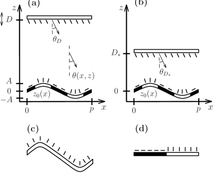
Figure 1: (a) The system under consideration consists of a nematic liquid crystal confined between two substrates at a mean distance $D$. The upper flat substrate induces strong anchoring, i.e., $\theta(x,z=D)=\theta_{D}$, while the lower substrate is characterized by a surface pattern of period $p$ in $x$ direction. The system is translational invariant in $y$ direction perpendicular to the plane of the figure. In (a) the lower sinusoidally grating surface (groove depth $A$) is endowed with an alternating stripe pattern of locally homeotropic anchoring (white bars) and homogeneous planar anchoring (black bars). The period of the chemical pattern is half the period of the surface grating $p$. In (c) and (d) a pure geometrically structured lower substrate and pure chemically patterned lower substrate, respectively, are shown. The anchoring direction at the substrates is schematically represented by black rods. Quantitatively reliable predictions of the phase behavior of a nematic liquid crystal confined between two substrates at an arbitrary mean distance $D$ in (a) can be achieved if the effective free energy function [Eqs. (6) - (II.3)] is analyzed. To this end the free energy functional of the nematic liquid crystal confined between two substrates at a single and rather small mean distance $D_{*}$ in (b) has to be minimized as is discussed in the main text.

$$F_{s}[\theta(x,z_{0}(x))]=$$ (5)

$$\!\!\!\!\!\frac{L}{2}\int^{p}_{0}dx\,w(x)\frac{\left(-\sin(\theta_{0}(x))z^{\prime}_{0}(x)+\cos(\theta_{0}(x))\right)^{2}}{\sqrt{1+(z^{\prime}_{0}(x))^{2}}},$$

where $\theta_{0}(x)\equiv\theta(x,z=z_{0}(x))$. Equations (4) and (5) together with the boundary condition for the nematic director at the upper surface completely specify the free energy functional for the system under consideration. The Euler-Langrange equations resulting from the stationary conditions of the total free energy with respect to the nematic director field can be solved numerically on a sufficiently fine two-dimensional grid using an iterative method. In order to obtain both stable and metastable configurations, different types of initial configurations are used. However, due to the pattern of the lower surface the determination of the director field and the phase diagram turns out to be a challenging numerical problem in particular in the case of large cell widths $D$. Moreover, the energy barrier between two metastable states cannot be determined this way.

II.3 Effective free energy function

Here we map the free energy functional $F[\theta(x,z);\theta_{D},D]$ [Eq. (4)] of a nematic liquid crystal cell with arbitrary width $D$ and arbitrary anchoring angle $\theta_{D}$ at the upper surface (see Fig. 1 (a)) onto the effective free energy function

$$F^{(eff)}(\tilde{\theta}_{0},\theta_{D},D) \!\!=\!\! \frac{KLp}{2D}\left(\theta_{D}-\tilde{\theta}_{0}\right)^{2}\!+\!F_{s}^{(eff)}(\tilde{\theta}_{0}),$$ (6)

where the average surface director orientation $\tilde{\theta}_{0}$ poni:97 at the lower patterned surface is given by

$$\tilde{\theta}_{0}(\theta_{D_{*}},D_{*}) = \theta_{D_{*}}-\frac{D_{*}}{KLp}\frac{\partial}{\partial\theta_{D_{*}}}F(\theta_{D_{*}},D_{*})|_{min}\,.$$ (7)

The effective surface free energy function $F_{s}^{(eff)}$ characterizing the anchoring energy at the patterned surface can be written as

$$F_{s}^{(eff)}(\tilde{\theta}_{0}(\theta_{D_{*}},D_{*}),D_{*})=$$

$$F(\theta_{D_{*}},D_{*})|_{min}-\frac{KLp}{2D_{*}}\left(\theta_{D_{*}}-\tilde{\theta}_{0}(\theta_{D_{*}},D_{*})\right)^{2}.$$

In order to calculate $\tilde{\theta}_{0}$ and $F_{s}^{(eff)}$ explicitly, we first determine numerically the minimum of the free energy $F(\theta_{D_{*}},D_{*})|_{min}$ of the nematic liquid crystal cell for a single and rather small value $D=D_{*}$ and arbitrary anchoring angle $\theta_{D_{*}}$ at the upper surface (see Fig. 1 (b)). Thereafter the phase behavior, energy barriers between metastable states, and effective anchoring angles for the system of interest (Fig. 1 (a)) can be obtained for arbitrary values of $D$ and $\theta_{D}$ from $F^{(eff)}(\tilde{\theta}_{0},\theta_{D},D)$ as a function of the single variable $\tilde{\theta}_{0}$. Such a calculation is considerably less challenging than minimizing the original free energy functional $F[\theta(x,z);\theta_{D},D]$ with respect to $\theta(x,z)$ on a two-dimensional $(x,z)$ grid. However, the effective free energy method is applicable only if Eq. (7) can be inverted in order to obtain $\theta_{D_{*}}(\tilde{\theta}_{0})$ which is needed as input into Eq. (II.3). The condition for this inversion follows from Eq. (7):

$$\left(1-\frac{D_{*}}{KLp}\frac{\partial^{2}}{\partial\theta^{2}_{D_{*}}}F(\theta_{D_{*}},D_{*})|_{min}\right)^{2}>0\,.$$ (9)

Moreover, $F_{s}^{(eff)}(\tilde{\theta}_{0}(\theta_{D_{*}},D_{*}),D_{*})$ is practically independent of the cell width $D_{*}$ provided $D_{*}\gtrsim p$ implying that the interfacial region above the lower substrate does not extend to the upper substrate.

Before studying the nematic liquid crystal in contact with the patterned substrates shown in Fig. 1 it is instructive to analyze first the nematic liquid crystal confined between two homogeneous flat substrates at a distance $D$. The upper surface induces strong anchoring, i.e., $\theta(z=D)=\theta_{D}$. The free energy functional defined in Eq. (4) follows as

$$F[\theta(z);\theta_{D},D] \!\!=\!\! \frac{KLp}{2}\int\limits_{0}^{D}dz\,\left(\frac{d\theta(z)}{dz}\right)^{2}+F_{s}(\theta_{0}).$$ (10)

The solution of the Euler-Langrange equation $\partial^{2}_{z}\theta(z)=0$ subject to the boundary condition at the upper surface $\theta(z=D)=\theta_{D}$ interpolates linearly between the top and bottom surfaces:

$$\theta(z) = \theta_{D}-\frac{1}{D}(D-z)(\theta_{D}-\theta_{0})\,,$$ (11)

where $\theta(z=0)=\theta_{0}$ follows from the boundary condition at the lower surface. With this solution of the Euler-Lagrange equation the minimized free energy function reads

$$F(\theta_{D_{*}},D_{*})|_{min} = \frac{KLp}{2D_{*}}\left(\theta_{D_{*}}-\theta_{0}\right)^{2}+F_{s}(\theta_{0})\,.$$

It follows directly from Eqs. (6) - (II.3) that $\tilde{\theta}_{0}=\theta_{0}$, $F_{s}^{(eff)}=F_{s}$, and

$$F^{(eff)}(\theta_{0};\theta_{D},D) = \frac{KLp}{2D}\left(\theta_{D}-\theta_{0}\right)^{2}+F_{s}(\theta_{0}).$$ (13)

Hence in the case of homogeneous confining substrates the effective free energy function [Eq. (13)] agrees exactly with the minimized free energy function of the original system [Eq. (II.3)].

III Applications

III.1 Geometrically and chemically patterned substrates

In the previous section we have shown that we can describe a nematic liquid crystal confined between two homogeneous substrates by the effective free energy function [Eq. (6)]. In this subsection we apply this approach to the particular case of a nematic liquid crystal confined between a chemically patterned sinusoidal surface and a flat substrate with strong homeotropic anchoring (see Fig. 1 (a)). The surface profile of the grating surface is given by $z_{0}(x)=A\sin\left(qx\right)$, where $A$ is the groove depth and $p=2\pi/q$ is the period. As Figure 1 (a) illustrates, the surface exhibits a pattern consisting of alternating stripes with locally homeotropic and homogeneous planar anchoring. The projection of the widths of the stripes onto the $x$ axis is $p/4$ and the anchoring strength is specified by a periodic step function: $w(x)=-w_{H}$ and $w_{P}$ for values of $x$ on the homeotropic and planar stripes, respectively. Figure 2 (a) displays $F(\theta_{D_{*}},D_{*}=p)|_{min}$ (dashed line) and $F_{s}^{(eff)}(\tilde{\theta}_{0},D_{*}=p)$ (solid line) for $pw_{H}/K=1$, $pw_{P}/K=2.5$, and $A/p=0.09$. The shapes of $F(\theta_{D_{*}},D_{*}=p)|_{min}$ as a function of $\theta_{D_{*}}$ and $F_{s}^{(eff)}(\tilde{\theta}_{0},D_{*}=p)$ as a function of $\tilde{\theta}_{0}$ are rather similar because $\tilde{\theta}_{0}\approx\theta_{D_{*}}$ (see Eq. (II.3)) for this set of model parameters. Figure 2 (b) displays the phase diagram plotted as a function of the anchoring angle $\theta_{D}$ at the upper substrate and the mean separation of the substrates $D$. The calculations demonstrate the existence of two (stable or metastable) nematic director configurations: the homeotropic (H) phase, in which the director field is almost uniform and parallel to the anchoring direction imposed at the upper surface, i.e., ${\hat{\bf n}}_{H}=(\sin\theta_{D},0,\cos\theta_{D})$, and the hybrid aligned nematic (HAN) phase, in which the director field varies from ${\hat{\bf n}}_{H}$ at the upper surface to nearly planar orientation through the cell. Note that there are two HAN textures: HAN₊ and HAN_- corresponding to positive and negative average surface angles at the lower surface (see also Fig. 7 below). For small anchoring angles $\theta_{D}$ the HAN phases are stable provided the cell width is larger than $D_{coex}$ (more precisely, the HAN₊ texture is stable for $\theta_{D}>0$ while the HAN_- texture is stable for $\theta_{D}<0$ and they coexist at $\theta_{D}=0$). For smaller distances between the substrates $D<D_{coex}$ the HAN phases are no longer stable because distortions of the director field are too costly in the presence of the dominating strong anchoring at the upper surface. The comparison of the phase boundary of thermal equilibrium as obtained from the effective free energy method [Eqs. (6) - (II.3), and solid line in Fig. 2 (b)] and the direct minimization of the underlying free energy functional [Eqs. (4) and (5), and diamonds in Fig. 2 (b)] demonstrate the reliability of the effective free energy method.

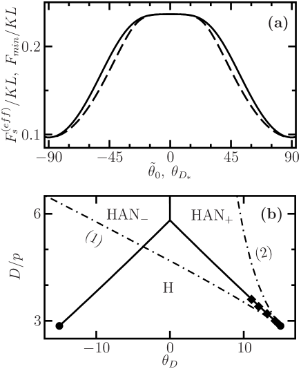
Figure 2: (a) The minimized free energy $F(\theta_{D_{*}},D_{*}=p)|_{min}$ (dashed line) and the effective surface free energy $F_{s}^{(eff)}(\tilde{\theta}_{0},D_{*}=p)$ (solid line) of a nematic liquid crystal confined between a flat surface with strong anchoring and a chemically patterned sinusoidal surface with groove depth $A/p=0.09$ (see Fig. 1 (b)). $L$ is the extension of the cell in the invariant $y$ direction, $K$ is the isotropic elastic constant, and the anchoring strength on the homeotropic stripes (white bars in Fig. 1 (b)) and planar anchoring stripes (black bars in Fig. 1 (b)) are $pw_{H}/K=1$ and $pw_{P}/K=2.5$, respectively. (b) Phase diagram of the same system as a function of the anchoring angle at the upper flat substrate $\theta_{D}$ and the cell width $D$ (see Fig. 1 (a)). The solid line denotes first order phase transitions between a homeotropic (H) and hybrid aligned nematic (HAN₊ and HAN_-) phases. At $\theta_{D}=0$ and $D/p\approx 5.8$ there is a triple point where the HAN₊, HAN_-, and H states coexist. The solid circle marks the critical point at $D_{cr}/p\approx 3$ and $\theta_{D}^{(cr)}\approx\pm 15^{\circ}$. The limits of metastability of the HAN₊ (1) and the H (2) state are denoted by the dot-dashed lines. The limit of metastability of the H state for $\theta_{D}<0$ and the HAN_- state are not shown for clearness. The lines and the solid circle follow from analyzing the effective free energy function [Eqs. (6) - (II.3)] while the diamonds represent the phase boundary of thermal equilibrium as obtained from a direct minimization of the underlying free energy functional [Eqs. (4) and (5)].

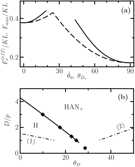
Figure 3: (a) The minimized free energy $F(\theta_{D_{*}},D_{*}=p)|_{min}$ (dashed line) and the effective surface free energy $F_{s}^{(eff)}(\tilde{\theta}_{0},D_{*}=p)$ (solid line) of a nematic liquid crystal confined between a flat surface with strong anchoring and a chemically patterned sinusoidal surface with groove depth $A/p=0.09$ (see Fig. 1 (b)). The anchoring strength on the homeotropic stripes and planar anchoring stripes are $pw_{H}/K=2.5$ and $pw_{P}/K=6$, respectively. (b) Phase diagram of the same system as a function of the anchoring angle at the upper flat substrate $\theta_{D}$ and the cell width $D$ (see Fig. 1 (a)). The solid line denotes the first order phase transition between a homogeneous (H) and hybrid aligned nematic (HAN₊) phase. The solid circle marks the critical point at $D_{cr}/p\approx 0.4$ and $\theta_{D}^{(cr)}\approx 29^{\circ}$. The limits of metastability of the HAN₊ (1) and the H (2) state are denoted by the dot-dashed lines. The lines follow from analyzing the effective free energy function [Eqs. (6) - (II.3)] while the diamonds and the solid circle represent the phase boundary and a critical point as obtained from a direct minimization of the underlying free energy functional [Eqs. (4) and (5)]. For $D\lesssim p$ the phase transition as well as the limits of metastability cannot be determined using the effective free energy function because $F_{s}^{(eff)}(\tilde{\theta}_{0})$ is not known in the region close to its maximum. For clearness, only the phase diagram for positive $\theta_{D}$ is shown (c.f. Fig. 2).

We note that the phase transition between the H and HAN textures is first order despite the fact that the effective surface free energy favors monostable planar anchoring, i.e., $F_{s}^{(eff)}$ exhibits only a minimum at $\tilde{\theta}_{0}=\pi/2$ in the interval $\tilde{\theta}_{0}\in[0,\pi/2]$. A first order phase transition in a nematic liquid crystal device with a monostable anchoring condition on a homogeneous lower substrate has been predicted for the special case $\theta_{D}=0$ in Refs. parr:03 ; parr:04 using the empirical expression

$$F_{s}(\theta_{0}) = \frac{w_{0}}{2}\sin^{2}(2\theta_{0})+w_{1}\sin^{2}(\theta_{0})$$ (14)

as input into Eq. (13). For $w_{1}<2w_{0}$ this surface free energy has two minima at $\theta_{0}=0$ and $\theta=\pi/2$ in the interval $\theta_{0}\in[0,\pi/2]$, and as such is bistable, while for $w_{1}>2w_{0}$, only the minimum $\theta_{0}=0$ exists, i.e., the surface is monostable. To study the stability limit of the H phase we expand $F^{(eff)}(\theta_{0})$ in Eq. (13) around $\theta_{0}=0$ up to sixth order:

$$F^{(eff)}(\theta_{0}) \approx F_{s}(0)+\frac{1}{2}\left(\frac{KLp}{D}+F_{s}^{{}^{\prime\prime}}(0)\right)\theta_{0}^{2}$$ (15)

$$+\frac{1}{4!}F_{s}^{(4)}(0)\theta_{0}^{4}+\frac{1}{6!}F_{s}^{(6)}(0)\theta_{0}^{6}\,.$$

The H phase corresponds to a local minimum of $F^{(eff)}(\theta_{0})$ in Eq. (13) if $D<D_{cr}$, where

$$D_{cr}=-\frac{KLp}{F^{{}^{\prime\prime}}_{s}(0)}\,.$$ (16)

A standard bifurcation analysis reveals that the transition from the H phase to the HAN phase can be either first order or continuous. The transition is continuous if $F_{s}^{(4)}(0)>0$, first order if $F_{s}^{(4)}(0)<0$, and $F_{s}^{(4)}(0)=0$ corresponds to a tricritical point. In the case of a first order phase transition the phase boundary of thermal equilibrium is given by

$$\frac{KLp}{D_{tr}}=\frac{10\left(F_{s}^{(4)}(0)\right)^{2}}{16F_{s}^{(6)}(0)}-F_{s}^{{}^{\prime\prime}}(0)\,.$$ (17)

We emphasize that the order of the phase transition depends only on the surface free energy $F_{s}(\theta_{0})$ close to $\theta_{0}=0$ for $\theta_{D}=0$. Therefore it is possible to have a first order phase transition even with a monostable surface characterized by a monotonic surface free energy such as the one shown in Fig. 2 (a) for ${\tilde{\theta}}_{0}\in[0,\pi/2]$ or the empirical equation (14) with $w_{1}>2w_{0}$ as well the more general expression four:99a

$$F_{s}(\theta_{0}) = \sum\limits_{n=0}^{\infty}\left[a_{n}\cos(2n\theta_{0})+b_{n}\sin(2n\theta_{0})\right]$$ (18)

with appropriate parameters $a_{n}$ and $b_{n}$.

First order phase transitions between the H and HAN texture are of particular interest for bistable liquid crystal displays. In a bistable liquid crystal display the two molecular configurations corresponding to light and dark states are locally stable in the thermodynamic space when the applied voltage is removed davi:02 ; harn:06 . Therefore, power is needed only to switch from one stable state to another, in contrast to monostable liquid crystal displays which require power to switch and to maintain the light and the dark states.

We now turn our attention to the case that it is not possible to evaluate $\theta_{D_{*}}(\tilde{\theta}_{0},D_{*})$ from $\tilde{\theta}_{0}(\theta_{D_{*}},D_{*})$ [Eq. (7)] because the condition for this inversion is not satisfied [Eq. (9)]. To this end we have chosen the parameters $pw_{H}/K=2.5$, $pw_{P}/K=6$, and $A/p=0.09$ for the system shown in Fig. 1 (a). Figure 3 (a) display $F(\theta_{D_{*}},D_{*}=p)|_{min}$ (dashed line) and $F_{s}^{(eff)}(\tilde{\theta}_{0},D_{*}=p)$ (solid line) while the corresponding phase diagram is shown in Fig. 3 (b). As is apparent from the solid line in Fig. 3 (a) it is not possible to determine the effective surface free energy function for the all values of $\tilde{\theta}_{0}$ because the upper flat substrate at $D_{*}$ is too far away from the lower patterned substrate in order to induce all possible average anchoring orientations $\tilde{\theta}_{0}$. In other words, the anchoring energy at the patterned substrate is too large to be balanced by the elastic energy for the chosen mean distance $D_{*}$ between the substrates (see Fig. 1 (b)). Nevertheless Fig. 3 (b) demonstrates that even this partial information about the effective surface free energy function can be used to calculate the phase diagram for cell widths sufficiently larger than the width at the critical point $D_{cr}$.

III.2 Purely geometrically structured substrates

In the last subsection we have shown that with a suitable chemical and geometrical surface morphology on one of the interior surfaces of a liquid crystal cell, two stable nematic director configurations can be supported. The zenithally bistable nematic devices that have been studied recently parr:03 ; brow:04 ; parr:04 ; parr:05 consist of a nematic liquid crystal confined between a chemically homogeneous grating surface (see Fig. 1 (c)) and a flat substrate with strong homeotropic anchoring. The profile of the asymmetric surface grating is given by

$$z_{0}(x)=A\sin\left(qx+h\sin(qx)\right),$$ (19)

where $A$ is the groove depth, $p=2\pi/q$ the period, and $h$ is the “blazing” parameter describing the asymmetry of the surface profile. Such a grating surface has been studied by Brown et al. brow:00 who found a first order transition between the HAN state, characterized by a low pretilt angle ($\tilde{\theta}_{0}\approx\pi/2$), and the H state, characterized by a high pretilt angle ($\tilde{\theta}_{0}\approx 0$). Strictly speaking, the H state does not correspond to the homeotropic texture (see Fig. 6 (b) below), but we keep the same notation as in the previous section for consistency. Here we study phase transitions of a nematic liquid crystal in contact with the blazed surface in a more detail using the effective free energy method discussed in Sec. II C.

In Fig. 4 (a) the minimized free energy $F(\theta_{D_{*}},D_{*}=p)|_{min}$ (dashed line) and the calculated effective surface free energy $F_{s}^{(eff)}(\tilde{\theta}_{0},D_{*}=p)$ (solid line) are shown for the anchoring strength $pw_{H}/K=2$ on the grating surface, the groove depth $A/p=0.27$, and the blazing parameter $h=0.2$. The effective surface free energy is asymmetric with respect to ${\tilde{\theta}}_{0}=0$ because of the asymmetry of the grating surface. As a consequence also the phase diagram, plotted as a function of the anchoring angle on the upper surface $\theta_{D}$ and the distance $D/p$ is asymmetric (Fig. 4 (b)). However, the topology of the phase diagram is the same as in the case of a symmetric substrate (see Figs. 2 (b), 3 (b), and for a more general discussion Sec. III C below).

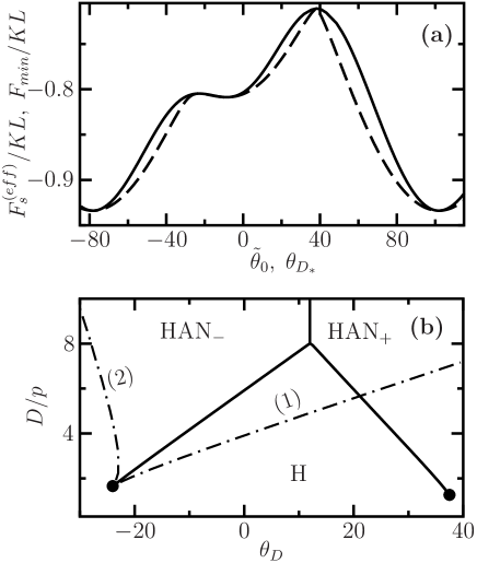
Figure 4: (a) The minimized free energy $F(\theta_{D_{*}},D_{*}=p)|_{min}$ (dashed line) and the effective surface free energy $F_{s}^{(eff)}(\tilde{\theta}_{0},D_{*}=p)$ (solid line) of a nematic liquid crystal confined between a flat surface with strong anchoring and a chemically uniform blazed surface (see Fig. 1 (c) and Eq. (19)). The locally homeotropic anchoring strength on the blazed surface is $pw_{H}/K=2$, the groove depth is $A/p=0.27$ and the blazing parameter is $h=0.2$. $L$ is the extension of the cell in the invariant $y$ direction and $K$ is the isotropic elastic constant. The effective surface free energy $F_{s}^{(eff)}$ (as well as $F(\theta_{D_{*}},D_{*}=p)|_{min}$) is periodic with the period $2\pi$ but it is asymmetric with respect to $\tilde{\theta}_{0}=0$. (b) Phase diagram of the same system as a function of the anchoring angle at the upper flat substrate $\theta_{D}$ and the cell width $D$ with the same line code as in Figs. 2 and 3. The triple point (where the HAN₊, HAN_- and H phases coexist) is at $\theta_{D}\approx 12^{\circ}$ and $D/p\approx 8$, and the critical points (solid circle) are at $D_{cr}/p\approx 1.3$, $\theta_{D}^{(cr)}\approx 38^{\circ}$ and $D_{cr}/p\approx 1.7$, $\theta_{D}^{(cr)}\approx-24^{\circ}$. For clearness, only the limits of metastability of the HAN_- (1) phase and the H (2) phase (for negative $\theta_{D}$) are shown.

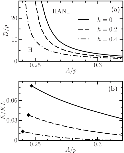
Figure 5: (a) The phase diagram of a nematic liquid crystal confined between the blazed surface (see Fig. 1 (c) and Eq. (19)) with local homeotropic anchoring and a flat surface with strong homeotropic anchoring ($\theta_{D}=0$) as a function of the groove depth $A/p$ and the cell width $D/p$. The anchoring strength on the blazed surface is $pw_{H}/K=2$. The lines correspond to different values of $h$ and denote first order transitions between homeotropic (H) and hybrid aligned (HAN_-) phases. For small $A/p$, the lines extend to $D=\infty$ corresponding to a first order anchoring transition between planar and homeotropic phases. Upon increasing $A/p$ the first order transition lines end at critical points which are not shown in the figure. (b) The energy barrier at the first order transitions with the same line code as in (a). The lines have been obtained from the total effective free energy (see Eq. (6)), while the diamonds correspond to the energy barriers between the planar and homeotropic effective anchoring which follow from considering only the surface contribution $F_{s}^{(eff)}$.

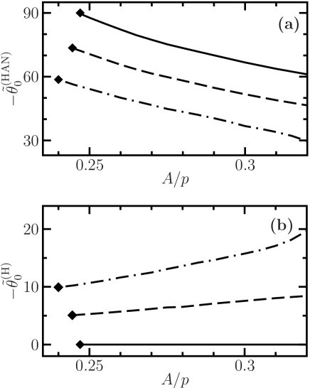
Figure 6: The average surface director (see Eq. (7)) for the hybrid aligned (HAN_-) phase in (a) and the homeotropic (H) phase in (b) on the lines of the first order transitions (see Fig. 5) for a nematic liquid crystal confined between the blazed surface (see Fig. 1 (c) and Eq. (19)) with local homeotropic anchoring and a flat surface with strong homeotropic anchoring ($\theta_{D}=0$). The diamonds in (a) and (b) correspond to the two minima of the effective surface energy function $F_{s}^{(eff)}(\tilde{\theta}_{0})$. The model parameters and the line code are the same as in Fig. 5.

We now concentrate on the most interesting (from a practical point of view) case of strong homeotropic anchoring ($\theta_{D}=0$) at the upper homogeneous surface. Figure 5 (a) displays the phase diagram for a few values of the blazing parameter $h$ and a fixed value of the local homeotropic anchoring strength on the grating surface $pw_{H}/K=2$. For a fixed cell width $D/p$, asymmetry ($h\neq 0$) leads to a decrease of the groove depth $A/p$ at which there is a first order transition between the HAN and the H phases, as compared to the nematic liquid crystal cell with the symmetric surface grating ($h=0$). Upon increasing the groove depth $A/p$ the transition line ends at a critical point (not shown in the figure), while it diverges as $A\to A_{0}$. The groove depth $A_{0}$ corresponds to an anchoring (or surface) transition between low tilt and high tilt surface states which are the homeotropic and planar effective anchoring states, respectively, in the case $h=0$.

The effective free energy method allows one to calculate an energy barrier $E$ between the two bistable states, which is not feasible by the direct numerical minimization of the free energy functional. The results of our calculations are shown in Fig. 5 (b). The asymmetry of the surface grating leads to a decrease of the energy barrier. With increasing groove depth $A/p$ the energy barrier decreases and eventually vanishes upon approaching the critical point. The diamonds in Fig. 5 (b) denote the energy barriers for the abovementioned anchoring transitions of a nematic liquid crystal in contact with a single grating surface.

The energy barrier between two bistable states is an important quantity for the design of a zenithally bistable nematic device. Too small energy barrier, as compared to $k_{B}T$, would cause spontaneous switching between the two states because of thermal fluctuations, while enlarging the energy barrier leads to an increase of the power consumption. Using the calculated values of $E$ (see Fig. 5 (b)) one can estimate the energy barrier in a real nematic liquid crystal cell. For instance, for a cell of area $1\,\mu\mathrm{m}\times 1\,\mu\mathrm{m}$ and of width $D=5\,\mu\mathrm{m}$, and taking the typical values $K=5\times 10^{-12}\,\mathrm{N}$ and $w_{H}=10^{-5}\,\mathrm{N/m}$, one obtains $E\approx 37\,k_{B}T$ for $h=0.2$ and $A\approx 0.026\,\mu\mathrm{m}$, which seems to be an acceptable value.

Another important quantity in zenithally bistable nematic devices is the average director orientation at the grating surface in the two degenerate states. The average surface director in the HAN ($\tilde{\theta}_{0}^{(\mathrm{HAN})}$) and H ($\tilde{\theta}_{0}^{(\mathrm{H})}$) states is shown in Fig. 6 for the same model parameters as in Fig. 5 and for the values of $A/p$ and $D/p$ corresponding to the coexistence line. The asymmetry of the surface grating leads to a decrease of $\tilde{\theta}_{0}^{(\mathrm{HAN})}$ and an increase of $\tilde{\theta}_{0}^{(\mathrm{H})}$. For a fixed value of $h$, the difference between the two angles decreases with increasing the groove depth $A/p$ and finally vanishes upon approaching the critical point (not shown in the figure).

Hence the asymmetry of the surface grating leads to a decrease of the groove depth at which the bistability is observed, which improves optical properties krie:02 , and to a decrease of the energy barrier, which lowers the power consumption of a zenithally bistable nematic device. On the other hand, also the difference between the two bistable states decreases which impairs optical properties of such a device.

III.3 Phase diagrams for a model surface free energy

In section III.1 we have discussed phase diagrams in the $(\theta_{D},D/p)$ plane which can be described in terms of the surface free energy given by Eq. (14). However, it is instructive to consider a more general situation that the surface free energy follows from a truncation of the Fourier expansion given in Eq. (18). To be able to study both symmetric and asymmetric surfaces we assume a natural generalization of Eq. (14), namely

$$F_{s}(\theta_{0})=\sum_{n=0}^{2}\left[a_{n}\cos(2n\theta_{0})+b_{n}\sin(2n\theta_{0})\right]\,,$$ (20)

which reduces to Eq. (14) in the case of a symmetric surface characterized by $b_{n}=0$. The angle $\theta_{0}^{(min)}$ that minimizes $F^{(eff)}(\theta_{0};\theta_{D},D)$ (see Eq. (13)) is a function of $\theta_{D}$ and $D$. The derivative

$$\chi=\left(\frac{\partial\theta_{0}^{(min)}}{\partial\theta_{D}}\right)_{D}=\frac{KLp/D}{KLp/D+F_{s}^{\prime\prime}(\theta_{0}^{(min)})},$$ (21)

is the susceptibility of the system that diverges at the critical thickness

$$D_{cr}=-KLp/\min_{\theta_{0}}F_{s}^{\prime\prime}(\theta_{0}),$$ (22)

and remains finite and positive for $D<D_{cr}$. From Eq. (22) the conditions for the critical angle $\theta_{0}^{(cr)}$ follow as

$$F_{s}^{(3)}(\theta_{0}^{(cr)})=0\;\;\;\textrm{and}\;\;\;F_{s}^{(4)}(\theta_{0}^{(cr)})>0\,,$$ (23)

implying that $D_{cr}$ and $\theta_{0}^{(cr)}$ depend only on the form of $F_{s}(\theta_{0})$.

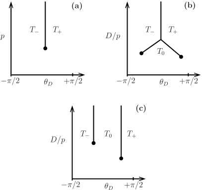
Figure 7: Schematic presentation of possible types of the phase diagram in the $(\theta_{D},D/p)$ plane for the surface free energy given by Eq. (20). $T_{0}$ and $T_{\pm}$ denote different (usually non-uniform) textures, the thick lines correspond to first order transitions, and black circles mark critical points. When $F_{s}$ (defined on the unit circle $z={\rm e}^{2i\theta_{0}}$) has one minimum and one maximum the phase diagram can be either of type (a) or (b). When $F_{s}$ has two minima and two maxima the phase diagram is of type (b) unless the minima are of equal depth, in which case it is of type (c). Note that the lines $\theta_{D}=\pm\pi/2$ are identified with each other and the phase diagram can be considered as being on a cylindrical surface.

The extremes of $F_{s}$ given by Eq. (20) can be found easily only in the case of symmetric or antisymmetric ($a_{n}=0$) surface and the same concerns the position of critical point. In this work, however, we are interested rather in possible topologies of the phase diagram in the $(\theta_{D},D/p)$ plane, which result from Eqs. (13) and (20), and not in the exact location of critical points or transition lines. To draw schematic phase diagrams we consider $F_{s}$ as a function defined on the unit circle $z={\rm e}^{2i\theta_{0}}$. Depending on the parameters $a_{n}$ and $b_{n}$, $F_{s}(\theta_{0})$ has either one minimum and one maximum or two minima and two maxima. This conclusion applies also to the function $F_{s}^{\prime\prime}(\theta_{0})$, thus, there can be either one or two critical points in the phase diagram (see Eqs. (22) and (23)). In the limit of large $D$, there is always a first order phase transition between two non-uniform textures corresponding to the opposite orientations of the director at $z=0$. This is because $F^{(eff)}$ is not a periodic function of $\theta_{0}$ at fixed $\theta_{D}$. To find $\theta_{D}$ at the transition we expand $F_{s}$ around its deepest minimum (denoted $\theta_{m}$), which leads to the approximate free energy:

$$F^{(eff)}(\theta_{D},D)|_{min}\approx F_{s}(\theta_{m})+\frac{KLp(\theta_{D}-\theta_{m})^{2}}{2(D+b)},$$ (24)

where $b=KLp/F_{s}^{\prime\prime}(\theta_{m})$ is the extrapolation length. Since $\theta_{m}$ and $\theta_{m}\pm\pi$ are equivalent minima of $F_{s}$, and both $\theta_{m}$ and $\theta_{D}$ are allowed to vary in the interval $[-\pi/2,\pi/2]$, the transition occurs at $\theta_{D}^{(tr)}=\theta_{m}+\pi/2$ if $-\pi/2\leq\theta_{m}\leq 0$ or at $\theta_{D}^{(tr)}=\theta_{m}-\pi/2$ if $0\leq\theta_{m}\leq\pi/2$. With the above information we can now draw schematically the phase diagram (see Fig. 7). Since the vertical lines at $\theta_{D}=\pm\pi/2$ are to be identified with each other the phase diagram can be considered on a cylindrical surface. Away from the transition lines there is a smooth evolution from one texture to another. This means that at fixed $D$ it is possible to transform smoothly the $T_{+}$ texture into the $T_{-}$ texture, i.e., without crossing the transition line, even for $D>D_{cr}$. We note that in some range of parameters, the phase diagram for $F_{s}$ with one minimum is topologically indistinguishable from that for $F_{s}$ with two minima (Fig. 7 (b)); in both cases there are two critical points and a triple point. If $F_{s}$ has two equal minima (e.g., at $\theta_{0}=0$ and $\theta_{0}=\pm\pi/2$ in the case of symmetric surface) the triple point disappears and the first order transition lines extend to $D\to\infty$, as shown in Fig. 7 (c).

IV Summary

We have studied the phase behavior of a nematic liquid crystal confined between a flat and a patterned substrate (Fig. 1) using the Frank-Oseen model [Eq. (4)] and the Rapini-Papoular surface free energy [Eq. (5)]. An expression for the effective free energy function of the system [Eq. (6)] was derived by determining an effective surface free energy characterizing the anchoring energy at the patterned surface [Eq. (II.3)]. Using the effective free energy function, we have determined the phase behavior of the nematic liquid crystal confined between a flat surface with strong anchoring and a chemically patterned sinusoidal surface (Fig. 1 (a)), finding first order transitions between a homeotropic texture (H) and hybrid aligned nematic (HAN) textures (Figs. 2 (b) and 3 (b)). It is possible to have a first order phase transition even with a monostable surface characterized by a monotonic surface free energy function (Fig. 2 (a), ${\tilde{\theta}}_{0}\in[0,\pi/2]$). In addition we have performed direct minimizations of the original free energy functional [Eqs. (4) and (5)] on a two-dimensional grid and found remarkably good agreement with the phase boundaries resulting from the effective energy function analysis (Figs. 2 (b) and 3 (b)). Hence quantitatively reliable predictions of the phase behavior can be achieved using the effective free energy method.

Using this method, we have also studied the phase behavior (Fig. 4 (b)) of a nematic liquid crystal confined between a chemically uniform, asymmetrically grooved substrate (Fig. 1 (c) and Eq. (19)) with locally homeotropic anchoring and a flat substrate with strong homeotropic anchoring, which is a typical setup for a zenithally bistable nematic device parr:03 ; brow:04 ; parr:04 ; parr:05 . The asymmetry of the grating substrate leads to a decrease of the groove depth at which a first order transition between the H and HAN phases occurs (Fig. 5 (a)). Moreover, we have determined the energy barrier between the two coexisting states (Fig. 5 (b)). Our calculations show that the energy barrier decreases with increasing the asymmetry of the grating surface but it is well above $k_{B}T$ for a typical nematic liquid crystal cell. In addition, the average director orientation at the grating surface in two bistable states has been calculated (Fig. 6). The difference between the two bistable states vanishes with increasing substrate asymmetry, which has a negative effect on the optical properties of a zenithally bistable nematic device.

We have also generalized the model of the effective surface free energy considered by Parry-Jones et al. parr:03 ; parr:04 to the case of asymmetric structured substrates and obtained three possible types of the phase diagram in the plane spanned by the orientation of the director at the homogeneous surface and the thickness of the nematic cell. The asymmetry of the substrate causes only a shift of transition lines and critical points, compared to the symmetric case, but does not change the topology of the phase diagram. Finally, we have verified that this model allows one to reproduce qualitatively the phase diagram of a nematic liquid crystal confined between a homogeneous planar substrate and an asymmetrically grooved surface (Fig. 4 (b) and Fig. 7 (b)).

References

- (1) Surfaces and Interfaces of Liquid Crystals, edited by T. Rasing and I. Muševič (Springer, Berlin, 2004).
- (2) L. Harnau and S. Dietrich, in Soft Matter, edited by G. Gompper and M. Schick (Wiley-VCH, Berlin, 2007), Vol. 3, p. 159.
- (3) D. W. Berreman, Phys. Rev. Lett. 28, 1683 (1972).
- (4) S. Faetti, Phys. Rev. A. 36, 408 (1987).
- (5) G. Barbero, T. Beica, A. L. Alexe-Ionescu, and R. Moldovan, J. Phys. II (France) 2, 2011 (1992).
- (6) R. Barberi, M. Giocondo, G. V. Sayko, and A. K. Zvezdin, Phys. Lett. A 213, 293 (1996).
- (7) F. C. Cardoso and L. R. Evangelista, Phys. Rev. E 53, 4202 (1996).
- (8) T. Z. Qian and P. Sheng, Phys. Rev. Lett. 77, 4564 (1996).
- (9) T. Z. Qian and P. Sheng, Phys. Rev. E 55, 7111 (1997).
- (10) G. P. Bryan-Brown, C. V. Brown, I. C. Sage, and V. C. Hui, Nature 392, 365 (1998).
- (11) J.-B. Fournier and P. Galatola, Phys. Rev. Lett. 82, 4859 (1999).
- (12) J.-B. Fournier and P. Galatola, Phys. Rev. E 60, 2404 (1999).
- (13) V. Mocella, C. Ferrero, M. Iovane, and R. Barberi, Liq. Cryst. 26, 1345 (1999).
- (14) G. Barbero, G. Skačej, A. L. Alexe-Ionescu, and S. Žumer, Phys. Rev. E 60, 628 (1999).
- (15) C. V. Brown, M. J. Towler, V. C. Hui, and G. P. Bryan-Brown, Liq. Cryst. 27, 233 (2000).
- (16) S. Kondrat and A. Poniewierski, Phys. Rev. E 64, 031709 (2001).
- (17) B. Wen and C. Rosenblatt, Phys. Rev. Lett. 89, 195505 (2002).
- (18) B. Wen, J.-H. Kim, H. Yokoyama, and C. Rosenblatt, Phys. Rev. E 66, 041502 (2002).
- (19) P. Patrício, M. M. Telo da Gama, and S. Dietrich, Phys. Rev. Lett. 88, 245502 (2002).
- (20) S. Kondrat, A. Poniewierski, and L. Harnau, Eur. Phys. J. E 10, 163 (2003).
- (21) B. Zhang, F. K. Lee, O. K. C. Tsui, and P. Sheng, Phys. Rev. Lett. 91, 215501 (2003).
- (22) A. Poniewierski and S. Kondrat, J. Mol. Liq. 112, 61 (2004).
- (23) O. K. C. Tsui, F. K. Lee, B. Zhang, and P. Sheng, Phys. Rev. E 69, 021704 (2004).
- (24) L. Harnau, F. Penna, and S. Dietrich, Phys. Rev. E 70, 021505 (2004).
- (25) F. Batalioto, I. H. Bechtold, E. A. Oliveria, and L. R. Evangelista, Phys. Rev. E 72, 031710 (2005).
- (26) S. Kondrat, A. Poniewierski, and L. Harnau, Liq. Cryst. 32, 95 (2005).
- (27) H. Desmet, K. Neyts, and R. Baets, J. Appl. Phys. 98, 123517 (2005).
- (28) L. Harnau, S. Kondrat, and A. Poniewierski, Phys. Rev. E 72, 011701 (2005).
- (29) J. T. K. Wan, O. K. C. Tsui, H.-S. Kwok, and P. Sheng, Phys. Rev. E 72, 021711 (2005).
- (30) K. Kiyohara, K. Asaka, and H. Monobe, N. Terasawa, and Y. Shimizu, J. Chem. Phys. 124, 034704 (2006).
- (31) F. S.-Y Yeung, F.-C. Xie, J. T.-K. Wan, F. K. Lee, O. K. C. Tsui, P. Sheng, and H.-S. Kwok, J. Appl. Phys. 99, 124506 (2006).
- (32) T. J. Atherton and J. R. Sambles, Phys. Rev. E 74, 022701 (2006).
- (33) I. H. Bechtold, F. Batalioto, L. T. Thieghi, B. S. L. Honda, M. Pojar, J. Schoenmaker, A. D. Santos, V. Zucolotto, D. T. Balogh, O. N. Oliveria, and E. A. Oliveria, Phys. Rev. E 74, 021714 (2006).
- (34) G. D., Boyd, J. Cheng, and P. D. T. Ngo, Appl. Phys. Lett. 36, 556 (1980).
- (35) J. Cheng, R. N. Thurston, G. D. Boyd, and R. B. Meyer, Appl. Phys. Lett. 40, 1007 (1982).
- (36) I. Dozov, M. Nobili, and G. Durand, Appl. Phys. Lett. 70, 1179 (1997).
- (37) R. Barberi, M. Giocondo, J. Li, R. Bartolino, I. Dozov, and G. Durand, Appl. Phys. Lett. 71, 3495 (1997).
- (38) H. Bock, Appl. Phys. Lett. 73, 2905 (1998).
- (39) Z. Zhuang, Y. J. Kim, and J. S. Patel, Appl. Phys. Lett. 75, 3008 (1999).
- (40) J.-X. Guo, Z.-G. Meng, M. Wong, and H.-S. Kwok, Appl. Phys. Lett. 77, 3716 (2000).
- (41) C. Denniston and J. M. Yeomans, Phys. Rev. Lett. 87, 275505 (2001).
- (42) J.-H. Kim, M. Yoneya, J. Yamamoto, and H. Yokoyama, Appl. Phys. Lett. 78, 3055. (2001).
- (43) J.-H Kim, M. Yoneya, and H. Yokoyama, Nature 420, 159. (2002).
- (44) A. J. Davidson and N. J. Mottram, Phys. Rev. E 65, 051710 (2002).
- (45) S. H. Lee, K.-H. Park, T.-H. Yoon, and J. C. Kim, Appl. Phys. Lett. 82, 4215 (2003).
- (46) L. A. Parry-Jones, E. G. Edwards, S. J. Elston, and C. V. Brown, Appl. Phys. Lett. 82, 1476 (2003).
- (47) C. V. Brown, L. A. Parry-Jones, S. J. Elston, and S. J. Wilkins, Mol. Cryst. Liq. Cryst. 410, 945 (2004).
- (48) L. A. Parry-Jones, E. G. Edwards, and C. V. Brown, Mol. Cryst. Liq. Cryst. 410, 955 (2004).
- (49) L. A. Parry-Jones and S. J. Elston, J. Appl. Phys. 97, 093515 (2005).
- (50) F. Barmes and D. J. Cleaver, Phys. Rev. E 69, 061705 (2004).
- (51) D. Sikharulidze, Appl. Phys. Lett. 86, 033507 (2005).
- (52) N. Mizoshita, Y. Suzuki, K. Hanabusa, and T. Kato, Adv. Mater. 17, 692 (2005).
- (53) C. Uche, S. J. Elston, and L. A. Parry-Jones, J. Phys. D.: Appl. Phys. 38, 2283 (2005).
- (54) L. Harnau and S. Dietrich, Europhys. Lett. 73, 28 (2006).
- (55) F. Barmes and D. J. Cleaver, Chem. Phys. Lett. 425, 44 (2006).
- (56) C. Uche, S. J. Elston, and L. A. Parry-Jones, Liq. Cryst. 33, 697 (2006).
- (57) F. Schmid and D. Cheung, Europhys. Lett. 76, 243 (2006).
- (58) C. W. Oseen, Arkiv För Matematik, Astronomi Och Fysik 19, 1 (1925).
- (59) H. Zocher, Z. Anorg. Allg. Chem. 147, 91 (1925).
- (60) F. C. Frank, Discuss. Faraday Soc. 25, 19 (1958).
- (61) A. Rapini and M. Papoular, J. Phys. (France) Colloq. 30, C4-54 (1969).
- (62) A. Poniewierski and A. Samborski, Liq. Cryst. 23, 377 (1997).
- (63) E. E. Kriezis, C. J. P. Newton, T. P. Spiller, and S. J. Elston, Appl. Opt. 41, 5346 (2002).