A search for solar-like oscillations in K giants in the globular cluster M4

Abstract

Context. To expand the range in the colour-magnitude diagram where asteroseismology can be applied, we organized a photometry campaign to find evidence for solar-like oscillations in giant stars in the globular cluster M4.

Aims. The aim was to detect the comb-like $p$-mode structure characteristic for solar-like oscillations in the amplitude spectra. The two dozen main target stars are in the region of the bump stars and have luminosities in the range 50–140 $\thinspace{\rm L}_{\odot}$.

Methods. We collected 6160 CCD frames and light curves for about 14 000 stars were extracted. The frames consist of exposures in the Johnson $B$, $V$ and $R$ bands and were obtained at three different telescopes. Three different software packages were applied to obtain the lowest possible photometric noise level. The resulting light curves have been analysed for signatures of oscillations using a variety of methods.

Results. We obtain high quality light curves for the K giants, but no clear oscillation signal is detected. This is a surprise as the noise levels achieved in the amplitude spectra should permit oscillations to be seen at the levels predicted by extrapolating from stars at lower luminosities. In particular, when we search for the signature of oscillations in a large number of stars we might expect to see common features in the power spectra, but even here we fall short of having clear evidence of oscillations.

Conclusions. High precision differential photometry is possible even in very crowded regions like the core of M4. Solar-like oscillations are probably present in K giants, but the amplitudes are lower than classical scaling laws predict. The reasons may be that the lifetime of the modes are short or the driving mechanism is relatively inefficient in giant stars.

1 Introduction

Asteroseismology has made great progress in recent years due to improved observational techniques. Extremely stable spectrographs have been designed with the aim to detect exo-planets through Doppler shifts. These instruments have allowed for the unambiguous detection of $p$-modes in about a dozen solar-type stars (for a review see Kjeldsen & Bedding review (2004)). Although most results have been obtained for dwarf and subgiant stars, some giant stars have been shown to oscillate: $\xi$ Hya (G7III; Frandsen et al. xihya (2002)), $\epsilon$ Oph (G9.5III; De Ridder et al. 2006a ), and $\eta$ Ser (K0III; Barban et al. kgiants (2004)). Unambiguous detection of $p$-modes has so far been restricted to field stars in our immediate neighbourhood.

Döllinger et al. (messenger (2005)) found that field stars show radial velocity and photometric variability, which seems to increase with increasing luminosity. This could either be due to a combination of activity and granulation or pulsations, either self-excited (Mira-like) or driven by convective motions (solar-like). Similar evidence for increased variability has been found for stars in the globular cluster 47 Tucanae (Edmonds and Gilliland tuc47 (1996)).

Stellar clusters present a highly interesting prospect, due to the large number of stars collected in a limited field of view and additional constraints from cluster properties like relative age, metallicity, and evolutionary stage. Gilliland et al. (m67 (1993)) were the first to make a search for solar-like oscillations in the main sequence F-type stars in the open cluster M67. However, based on their multi-site campaign using 4-m class telescopes they made no clear detection. Recently, another campaign was carried out on the same cluster (Stello et al. 2006b ; stello07 (2007)), this time concentrating on stars on the lower part of the giant branch with expected larger oscillation amplitudes.

Knowing that $p$-modes are excited in giant stars, we decided to study K giants in the globular cluster M4. The two main reasons are that M4 has a rich population of K giants (see Fig. 2) and the amplitudes are expected to be substantially higher than for subgiants. The prospect is that if we can measure the gross properties of the oscillations, like amplitudes and the large splitting characteristic for solar-like oscillations, we could potentially study an ensemble of giant stars in different evolutionary stages.

According to the empirical calibration by Kjeldsen & Bedding (kandb (1995)) oscillation amplitudes scale as $L/(M\,T_{\rm eff}^{2})$. For the K giants in M4, taking the solar amplitude as 4.7 ppm (parts per million), we expected amplitudes in the range 400–1000 ppm. The noise level we expected to reach in the amplitude spectra for the bright giant stars was $\simeq\,25$ ppm at high frequencies. This would allow us to detect any excess power and possibly the comb-like structure of the $p$-modes in the amplitude spectra for the brightest and least crowded targets. The mode frequencies unfortunately decrease with luminosity and approach a range where noise caused by extinction and transparency changes is difficult to eliminate in ground-based data.

2 The observations

CCD frames were obtained with the Danish 1.54 m telescope at La Silla, the 1.5 m telescope at Cerro Tololo Inter-American Observatory (CTIO), both in Chile, and the 1 m telescope at the Siding Spring Observatory (SSO) in Australia. The observations took place over a period of almost three months in order to get the necessary frequency resolution. We started at La Silla on April 13, 2001 and got the last data on June 27, 2001. We obtained useful data on 48 nights out of an allocation of 63 nights. Some nights had overlap between Australia and Chile which can be used to check the consistency of the photometric results. Table 1 gives a list of the collected dataset. In total we have 6160 CCD frames of M4 (4014 from La Silla, 863 from CTIO, and 1283 from SSO).

In order to identify the mode type, we decided to observe in three filters $B$, $V$ and $R$. Amplitude ratios between different colours will indicate which type of modes are present. To enhance the signal to noise ratio the data can still be combined using an approximate scaling (Eq. 8) as phase differences of $p$-modes between filters are small. About equal time was allocated to the three filters giving more frames in $R$ due to the shorter exposure times.

Table 1: Observing log for the M4 campaign in 2001.

	Number of images			Date of observation
Observatory	$B$	$V$	$R$	Start	End
SSO	0	548	735	May 1	June 10
CTIO	143	274	446	June 1	June 6
La Silla	847	1358	1809	April 13	June 30

The time distribution is represented in Fig. 1, which includes 31 nights from La Silla, 6 nights from CTIO, and 11 nights from SSO.

Figure 1: Distribution of nights for the three observing sites. The time baseline is 78 days.

The exposure times were adjusted to give the best result for stars in the range $12.5<V<13.5$, which is the area of the RGB bump in M4 shown in Fig. 2. Typically this meant exposure times at La Silla and CTIO of less than a minute in $V$ and $R$ and a few minutes in $B$ depending on seeing conditions. Exposure times at SSO were 2–4 minutes in $V$ and 1–2 minutes in $R$. On average this led to a mean duty cycle around 50%, since the readout time was 1–2 minutes.

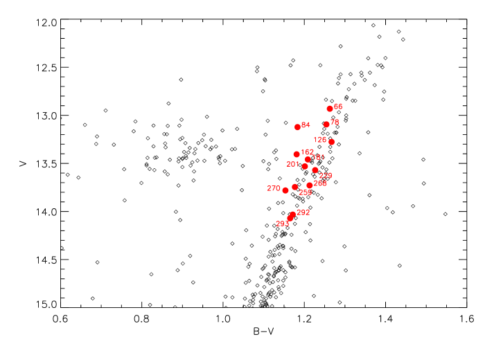
Figure 2: The colour-magnitude diagram for M4 showing the bump stars and part of the horizontal branch. The colours and magnitudes have been calibrated using the database provided by Stetson (stetson07 (2007)). To show the range covered, some of the stars selected for a detailed analysis are indicated and labeled with the ID – see Table 2.

3 CCD photometry techniques

The images were first calibrated by performing traditional bias subtraction and flat fielding. In order to avoid nightly offsets, calibration frames were constructed for periods of several days, typically a week, and the same calibration frames were used for all images in that period. This point is quite important since the timescale of variability for the giant targets is in the range 9–31 hours (cf. Sect. 5.1).

CCD non-linearity was considered, and in the case of the La Silla data the non-linearity was corrected by the technique described by Stello et al. (2006b ). The other cameras did not provide the same option for a correction and were assumed to be linear. We have not seen any evidence for non-linearity, and as we were able to find comparison stars with similar magnitudes in all cases, the influence of non-linearity should be negligible.

In Fig. 3 we present the calibrated CCD image, which has been used as the reference image for the La Silla observations of M4. The two dozen K giant stars we selected for a detailed analysis are marked by boxes.

Figure 3: The field of M4 observed with the Danish 1.54 m telescope at La Silla. The two dozen K giants we analysed in detail are marked by squares. The center of the field is at $\alpha_{2000}=16^{h}23^{m}33^{s}.7,\,\delta_{2000}=-26^{\circ}31^{\prime}05".7$.

In order to achieve the highest possible photometric precision we decided to use three different reduction programs, which have all been successful in the past in producing high quality results: isis, daophot and momf. In the most crowded areas we expected isis (Alard & Lupton isis98 (1998); Alard isis00 (2000)) to give the best results. In the less crowded areas we expected that daophot (Stetson stetson (1987)) would do best. Finally, we know that momf (Kjeldsen & Frandsen momf (1992)) performs very well in fields with only mild crowding. All frames were reduced with isis and daophot and a subset of the $V$ frames from La Silla were reduced with momf. Each of the three methods will be described in Sects. 3.1–3.3 and we compare the results in Sect. 3.4.

3.1 The image subtraction method (isis)

The main advantage of the difference-image technique is the ability to extract high precision photometry in the crowded regions near the core of M4. In addition, any variations due to airmass and transparency changes are removed to first order as a part of the image subtraction.

The image subtraction method isis (Alard & Lupton isis98 (1998); Alard isis00 (2000)) was used by two members of the team independently (isis1 and isis2). For each filter and each observing site we selected the images with the best seeing to make the reference images. While isis2 only used a single reference image for each site and filter, isis1 used subsets of data from about one week.

For each observed image, isis computed a kernel which describes the variations of the PSF across the image relative to the reference image. isis then convolves the reference image with the kernel and subtracts this from the observed image. The resulting difference image will contain the signal that is intrinsically different from the reference image, e.g. cosmic ray hits, hot pixels, and variable stars.

In the first approach (isis1) only La Silla and CTIO data were included (Bruntt bruntt_phd (2003)). They were divided into five subsets and reduced separately. The reason for this was large differences in the positional angle of the CCD camera between different periods. We had problems using the photometry package that is part of isis. Instead, we modified the aperture photometry routine in daophot in order to be able to run it on the subtracted images, in particular allowing negative flux values. The necessary modifications were described in detail by Bruntt et al. (bruntt6791 (2003)). isis needs a reference flux for each star, as only the change in the flux is calculated. This was taken from the daophot reduction of the reference images.

In the second reduction approach (isis2) we constructed only one reference frame (for every observing site and passband). The original isis software does not work correctly with frames that are significantly rotated with respect to the reference frame. The problem resides in the interpolation process. We used our own application, which performs this task correctly even for large rotation angles but requires much more computation time. For all stars detected in the reference frames (of all three observing sites) we derived differential fluxes from our CCD frames following standard procedure of isis reductions (for details see Kopacki kop2000 (2000)). We performed both the PSF fitting and aperture photometry on the difference frames. To transform differential fluxes into magnitudes we used total fluxes measured in the reference frames using aperture photometry tasks neda$+$daogrow under daophot. Finally, all the data were merged into a uniform magnitude system by applying magnitude offsets determined from a carefully chosen set of bright unsaturated stars common to all three observing fields. In this way, the CTIO and SSO data were transformed into the magnitude scale of the La Silla data.

Figure 4: The rms scatter around the mean for a good night with the Danish 1.54 m telescope for the isis1 reduction. The (red) squares give the noise level for the final time series for the selected K giants, where we have looked for solar-like oscillations. The line indicates the estimated noise from scintillation and photon statistics. The excess of stars with high noise near $V=13.3\pm 0.3$ are the RR Lyrae stars. Saturation sets in at $V\sim 12.5$.

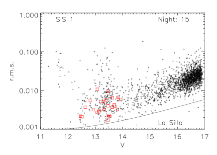
Figure 5: Same as Fig. 4, but for a bad night. The night is characterized by very large sky background contribution due to moon light.

3.2 daophot/allstar/allframe reduction

For the photometry we used the suite of photometry programs developed by Stetson (stetson (1987), stetson2 (1990), stetson3 (1994)): daophot, allstar and allframe. The general use of these is well described in manuals and the literature. For our applications we adopted a slightly modified procedure, which consisted in the following. Firstly, a few of the deepest and lowest-seeing frames were used to produce a master list of stars, which was obtained by several iterations through daophot, allstar and allframe. Next, all frames were run through daophot/allstar once. With the preliminary photometry in hand, positional transformations between each frame and our reference frame were derived using daomatch and daomaster (kindly provided by P. Stetson).

From the frames used to derive the master star list, we created two lists of stars for generating the PSF for the individual images. The first list contained $\sim$10 stars that were well isolated and these were used to generate the first version of the PSF for each frame. Next the second list, containing $\sim$200 stars covering the observed field, was used to generate the final PSF. We used this PSF when running allframe on all the images to produce the final photometry. We made a cross id of all stars in the photometry files and the 7,000 brightest stars were selected for further analysis.

3.3 momf reduction

As an independent test we used the momf package (Kjeldsen & Frandsen momf (1992)) on the La Silla images to derive time series in the $V$ band. The reduction had to be done in a slightly different way than normal, as the La Silla images were slightly rotated relative to each other. momf can only handle shifts. Thus we had to introduce an additional coordinate transformation changing the $(x,y)$ coordinates for each image before doing photometry. For stars outside the very crowded regions, results were comparable to the other techniques. We conclude that we reach similar results for non-crowded regions by all of the techniques.

3.4 Comparison of the photometry

Our database contains photometry from the three different reduction methods and comprises light curves of 13 611 stars with up to 6 160 data points. We also store information about each frame such as seeing, airmass, background level, the mid-time of each observation (Julian date), and position on the reference frame of each star. The data can be accessed at the web page http://astro.phys.au.dk/$\sim$srf/M4/.

The rms scatter in the light curves is plotted versus magnitude for a relatively good and bad night in Fig. 4 and 5, respectively. These results are based on the isis1 photometry in the $V$-band. For the bad night, the noise is considerably larger than the good night for all stars. The higher noise is due to high sky background as a result of the close proximity of the Moon to M4. The lower envelope of stars for the good night is close to the expected precision based on the flux level (indicated by the solid line). We find a number of stars with rms scatter as low as 1.5 mmag. For the K giants the level is typically about 2 mmag per data point. The bump stars are found around $V=13.5$, where we obtain the lowest noise levels.

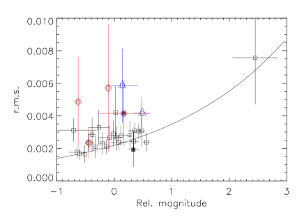
Figure 6: The mean rms scatter per data point per night is plotted against the nightly mean flux level in the exposures represented by a corresponding magnitude difference between each night and a reference night. The filled symbols are two nights with very few observations. The over-plotted diamonds indicate nights with a high sky level and the triangles nights with very good seeing. The rms uncertainty is marked for each point.

Figure 7: The mean scatter per data point per night for night 14 for the daophot (left panel) and isis1 reduction (right panel). The line gives the noise level for a good night, see Fig. 4.

As shown in Fig. 5, some nights do not give good results, with noise levels considerably higher than the majority of the data. Naturally, the noise per data point depends on the level of exposure per frame. This will vary as we had to adjust the exposure time to avoid saturation. In good seeing we obtained fewer photons per frame as the stellar image size is smaller and the maximum exposure level is kept constant to avoid saturation. Also, when cirrus clouds were present we kept the exposures times a bit conservative in order to avoid occasional over-exposed images from holes in the clouds.

We have investigated in which conditions the photometry was worse than expected from photon noise alone. To do this we considered the isis1 photometry of stars from La Silla. We selected an ensemble of 19 bright stars and calculated their average scatter per night. The average flux for the ensemble was also derived and converted to a magnitude. One good night was chosen as the reference night and the magnitude for that night was subtracted from the magnitudes from all other nights.

The measured rms scatter is plotted against the magnitude for all the nights in Fig. 6. If only photon noise were present the scatter should follow the solid line in Fig. 6, ie. following the relation: $5\,\log_{10}\sigma=m-m_{\rm ref}$.

Most of the nights follow this law, but there are exceptions. Nights with a high sky background clearly stand out as less valuable for the purpose of achieving high photometric precision (diamonds in Fig. 6). A second problem arises, when the seeing is very good since under-sampling sets in (triangles in Fig. 6).

An important issue is whether any of the three reduction techniques are superior. In general we find that the results are quite similar for the image subtraction, PSF fitting, and aperture photometry techniques. However, momf is clearly not suited for crowded fields and only for a small fraction of stars does it perform as well as isis or daophot. The quality of the daophot photometry is comparable to the isis results, although isis is superior in the most crowded areas. We also find the best results with isis for faint stars, especially on nights with bad seeing. This is shown in Fig. 7 where we compare the rms scatter in data from one bad night from La Silla using daophot (left panel) and isis (right panel). The rms noise of the K giant stars is 40% lower for the isis reduction.

It is possible that with a more careful choice of PSF stars and other parameters involved in the daophot reductions, it may be possible to improve these results. The optimum choice of parameters for good observing conditions might not be the best for frames obtained under non-photometric conditions.

A final illustration of the differences seen between the different algorithms is presented in Fig. 8. Here the rms scatter is presented for three different reductions: isis1, isis2 and daophot. Each point is for a particular star and the symbols define which reduction technique was being used. It is evident, that none of the techniques produce the best results in all cases. It seems that the image subtraction method isis1 has been most successful on average.

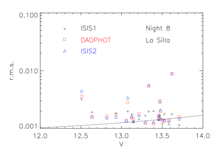
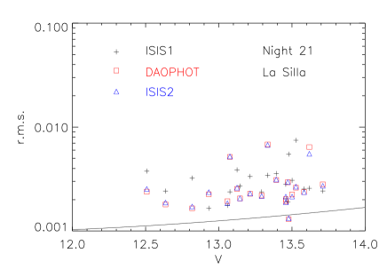
Figure 8: The rms noise level in K giant stars for La Silla data from two different nights is shown in the left and right panel. We compare the noise level from the three reduction methods. It is similar for most stars, but in a few cases the daophot and isis2 noise levels are higher than for isis1.

The time series from each observatory show different characteristics due to different observing conditions and different telescope and detector setups. At the SSO the seeing was considerably worse leading to more extended stellar images. This leads to increased noise as a result of the higher influence of the background level, which is worse for fainter stars. This effect is shown in Fig. 9. The CTIO data are heavily influenced by the presence of the Moon bing close to the target field, particularly in the middle of the run, and this makes the data of rather poor quality. The results can be characterized by the rms noise per data point for a non-crowded K giants for the three sites on a good night: $1.6$ mmag for La Silla, $3.0$ mmag for CTIO and $2.1$ mmag for SSO.

4 Light curve preparation

The outcome of the previous section is either absolute or differential magnitudes. In both cases it is necessary to make differential photometry by comparing each target star with a set of reference stars. The effects of extinction, instrumental drifts and other sources of non-stellar noise need to be minimized for us to be able to study and stellar signal at frequencies below $30$ $\mu$Hz corresponding to periods longer than 9 hours. The approach is described in the following Sections.

4.1 Ensemble photometry

An ensemble of reference stars is used to derive the relative magnitude for all stars. This should take out transparency and extinction variations. In M4 there is a wide range of possibilities for choosing reference stars. However, the results depend strongly on the implementation of the ensemble average performed.

The algorithm we employed was the following: for a given star, a number of reference stars were selected which were required to have similar $V$ magnitude and $B-V$ colour and be within a certain distance (eg. half the size of the CCD) on the CCD frame. We calculated the magnitude difference of the target star and each reference star for a whole observing block ($t\geq 7$ d) and subtracted the median value producing a time series $\Delta m_{i}(t)$, where the index $i$ indicate the reference star.

We now do an analysis night by night. For each night the rms noise $\sigma_{i,\rm rms}$ of each $\Delta m_{i}(t)$ time series is calculated and a weight is assigned using

$$w_{i}=1/\sigma_{i,\rm rms}^{2}.$$ (1)

The 10 stars with highest weights are used to calculate the final light curve for the night as the weighted sum

$$\Delta m(t)=\sum_{i=1}^{10}w_{i}\Delta m_{i}(t)/\sum_{i=1}^{10}w_{i}.$$ (2)

The set of reference stars will vary from night to night. The method does not imply any high-pass filtering at a timescale of one day, as the median is subtracted before splitting the time series into single nights. The technique gives slightly lower (10–20%) white noise levels in the final light curves compared with the simpler choice of a common set of reference stars extending over all nights of an observing period. The final light curves are obtained by selecting, for each observing site, the result with lowest noise among the different methods applied (daophot, isis1 and isis2).

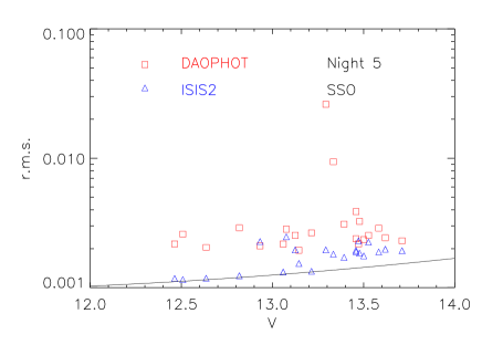
Figure 9: The rms noise levels in data from a good night at SSO. daophot is doing significantly worse than isis2. Notice the increased noise at faint magnitudes relative to the photon noise estimate (solid curve).

4.2 Decorrelation

Instrumental drifts and reduction noise may lead to correlation of the measured magnitudes with parameters like the colour of the star, position on the CCD and airmass. We found no clear correlations between the relative magnitudes and parameters like airmass, sky background or position on the CCD. As a consequence no type of decorrelation was performed.

4.3 Combining $B$,$V$ and $R$

The results from the procedures described in Sect. 4.1 are a set of light curves from the three sites in three filters $B$, $V$ and $R$. In our search for solar-like oscillations in the K giants we assume that phase shifts between observations in different filters are small (Jiménez et al. phases (1999)). We also assume that the oscillation amplitudes scale with inverse wavelength as $A\propto\lambda^{-1}$ (Eq. 8) and we therefore scaled the $B$ and $R$ time series relative to the $V$ filter: scaling factors were 1.222 and 0.846. The weights, described in the next subsection, were also scaled with the inverse factor following Eq. 4.

Table 2: The 24 K giants selected for detailed analysis. ID2 is from Stetson (stetson07 (2007)) if present in the catalog (NA means not available) and $V$ and $B-V$ are calibrated using this database. $T_{\rm eff}$ is found using the $B-V$ calibration of Alonso et al. (alonso (1999)) while the luminosity and radius were determined using the parameters for the M4 cluster (see text for details). In the last four columns we list the predicted values for the peak amplitude in ppm when assuming $\delta L/L\propto(L/M)^{0.7}$, $\nu_{\rm max}$ is the expected peak frequency for $p$-modes, $\Delta\nu_{0}$ is the large separation, and $\omega_{c}$ is the acoustic cutoff frequency (frequencies are all in $\mu$Hz and calculated from Eqs. 5–8).

ID	ID2	$\alpha_{2000}$	$\delta_{2000}$	$V$	$B-V$	$L$/$\thinspace{\rm L}_{\odot}$	$T_{\rm eff}$	$R$/$\thinspace{\rm R}_{\odot}$	$\delta L/L$	$\nu_{\rm max}$	$\Delta\nu_{0}$	$\omega_{c}$
66	364	16 23 53.65	-26 33 55.0	12.93	1.263	143.0	4723	17.9	254	8.9	1.64	16.4
78	1715	16 23 32.46	-26 26 20.7	13.09	1.254	123.1	4741	16.5	227	10.5	1.86	19.4
83	689	16 23 27.34	-26 30 59.1	13.03	1.303	130.3	4637	17.7	247	9.2	1.67	16.9
84	264	16 23 54.72	-26 31 22.6	13.12	1.183	120.0	4903	15.2	209	12.2	2.10	22.3
126	NA	16 23 26.94	-26 30 43.9	13.28	1.267	104.1	4714	15.3	204	12.2	2.07	22.4
162	986	16 23 50.23	-26 29 28.0	13.41	1.181	92.4	4909	13.3	173	15.8	2.56	29.1
166	1753	16 23 22.96	-26 30 32.6	13.44	1.221	89.3	4815	13.6	176	15.3	2.48	28.2
181	NA	16 23 50.01	-26 32 21.5	13.46	1.209	88.0	4844	13.3	172	15.9	2.55	29.2
195	NA	16 23 47.55	-26 31 06.0	13.47	1.218	86.9	4822	13.4	172	15.8	2.54	29.1
200	NA	16 23 19.94	-26 32 40.1	13.54	1.203	82.0	4856	12.8	163	17.2	2.71	31.6
201	NA	16 23 53.03	-26 28 09.1	13.53	1.201	82.4	4861	12.8	163	17.2	2.71	31.6
210	NA	16 23 43.11	-26 28 08.8	13.52	1.190	83.4	4888	12.8	163	17.3	2.73	31.8
228	NA	16 23 47.84	-26 29 50.2	13.56	1.196	80.5	4873	12.6	160	17.7	2.78	32.6
229	NA	16 23 45.01	-26 33 58.3	13.57	1.227	79.4	4803	12.9	163	17.1	2.68	31.4
243	NA	16 23 21.77	-26 26 45.8	13.59	1.205	77.9	4851	12.5	158	18.0	2.81	33.1
244	NA	16 23 24.57	-26 31 10.6	13.64	1.226	74.6	4805	12.5	156	18.2	2.82	33.5
259	243	16 23 42.43	-26 33 18.6	13.75	1.177	67.6	4919	11.3	139	21.8	3.26	40.1
266	NA	16 23 48.97	-26 29 21.3	13.70	1.278	70.8	4691	12.8	158	17.7	2.73	32.4
268	331	16 23 41.72	-26 29 47.9	13.73	1.213	68.6	4834	11.8	145	20.2	3.06	37.2
270	540	16 23 47.83	-26 32 44.7	13.78	1.153	65.4	4976	10.9	133	23.5	3.45	43.1
280	463	16 23 32.34	-26 29 22.4	13.82	1.172	63.0	4931	10.9	131	23.6	3.46	43.4
285	305	16 23 42.13	-26 32 07.4	13.83	1.233	62.7	4788	11.5	139	21.4	3.18	39.3
292	1005	16 23 26.05	-26 30 39.6	14.03	1.172	51.9	4931	9.9	115	28.7	4.00	52.7
293	1059	16 23 22.50	-26 29 41.2	14.07	1.165	50.1	4947	9.7	111	30.0	4.15	55.2

4.4 Removing outliers and weighting the data

Due to the changes in observing conditions there is a large variation in the data quality from night to night. It is therefore essential to apply weights when the Fourier spectra are calculated.

In the first step we remove obvious outliers. All points that deviate more than 5$\sigma$ from the mean are discarded. Weights are then calculated for each star by combining a weight for each night and a weight based on the point-to-point scatter. Each night gets a weight, which is

$$w_{1}=1/\sigma_{night}^{2},$$ (3)

where $\sigma_{night}$ is the rms noise of the time series for the entire night. All data points from this night get the same weight.

The point-to-point weight is calculated by first computing a spline fit to an averaged time series with a smoothing width of $\pm 0.075$ d. The spline fit is subtracted from the data. The noise level at any given point in time $\sigma_{pt}$ is then the average rms calculated using a Gaussian with a width of 0.05 d. The weight is chosen as the inverse of the noise level:

$$w_{2}=1/\sigma_{pt}.$$ (4)

We note that Eq. 4 (rather than use of inverse variance) was also the preferred weighting in similar multi-site campaigns by Handler (handler03 (2003)) and Bruntt et al. (brunttM67 (2007)).

The final weight we use is the product of $w_{1}$ and $w_{2}$. A maximum weight (4 times the mean weight) is defined to avoid nights with very few points to give very high weights.

5 Selection of K giant targets

We selected two dozen K giants for a detailed analysis. The stars are found in the least crowded parts of M4 and cover a range in luminosity on both sides of the bump stars. Further, we selected the stars with the rms scatter in the time series less than 4 mmag. We list their ID numbers, standard $V$ magnitude and $B-V$ colour in Table 2. The position of some of the stars in the colour-magnitude diagram is shown in Fig. 2 and the position in the cluster are marked with squares in Fig. 3.

To calculate $L$/$\thinspace{\rm L}_{\odot}$, $T_{\rm eff}$ and $R$/$\thinspace{\rm R}_{\odot}$ for the targets we used cluster parameters from Ivans et al. (ivans (1999)) for M4: distance $d=2.1$ kpc, reddening $E(B-V)=0.37$, interstellar absorption $A_{V}=4.0E(B-V)$, metal content [Fe/H]$=-1.2$, bolometric correction $BC=-0.48$ and mass $M=0.85\hbox{$\thinspace{\rm M}_{\odot}$}$. As pointed out by Ivans et al. (ivans (1999)), the reddening is varying over the field of the cluster. These parameters lead to a distance modulus of $(m-M)_{V}=13.1$. This compares reasonably well with the mean magnitude of the RR Lyrae stars (Kopacki & Frandsen, rrlyr (2007)) in the range $13.2$–$13.3$, which have absolute magnitude $M_{\rm V}\simeq 0.0$. The uncertainty of the cluster parameters introduce a $\sim$10% uncertainty in the luminosities.

5.1 Expected signal for solar-like oscillations

We have made estimates of the amplitude and frequency that is expected for solar-like oscillations.

We use the following scaling relations for the frequency separation $\Delta\nu_{0}$, the expected location of $p$-mode maximum frequency $\nu_{\rm max}$ and the acoustic cutoff frequency $\omega_{c}$:

$$\Delta\nu_{0}=134.9\,(M/\hbox{$\thinspace{\rm M}_{\odot}$})^{1/2}(R/\hbox{$\thinspace{\rm R}_{\odot}$})^{-3/2}\,\mu{\rm Hz},$$ (5)

$$\nu_{\rm max}=3050\,{M/\hbox{$\thinspace{\rm M}_{\odot}$}\over(R/\hbox{$\thinspace{\rm R}_{\odot}$})^{2}(T_{\rm eff}/5777\,{\rm K})^{0.5}}\,\mu{\rm Hz},$$ (6)

$$\omega_{c}=5600\,{(M/\hbox{$\thinspace{\rm M}_{\odot}$})\over(R/\hbox{$\thinspace{\rm R}_{\odot}$})^{2}(T_{\rm eff}/5777\,{\rm K})}\,\mu{\rm Hz}.$$ (7)

The expected amplitude of the oscillation modes were estimated from the calibration by Kjeldsen and Bedding (kandb (1995)), but using the scaling $\delta L/L\propto(L/M)^{0.7}$ suggested by Samadi et al. (samadi (2006)):

$$(\delta L/L)_{\lambda}=4.7\,{[(L/\hbox{$\thinspace{\rm L}_{\odot}$})\,/\,(M/\hbox{$\thinspace{\rm M}_{\odot}$})]^{0.7}\over(\lambda/550\,{\rm nm})\,(T_{\rm eff}/5777\,{\rm K})^{2}}\,{\rm ppm}.$$ (8)

The computed parameters using Eq. 5–8 for the 24 selected K giants are listed in Table 2. As the luminosity decreases from about 150 to 50 $L_{\odot}$ the amplitudes decreases from 300 to 100 ppm, while the frequency of maximum power shifts from 9 to 30 $\mu$Hz (periods of 31 to 9 hours). The search for the signatures of the oscillations will be difficult, as we are in the region of the frequency spectrum that is affected by slow drifts originating from observing conditions (seeing, transparency and extinction) and the instrument (eg. slight changes in the position of the stars on the CCD).

6 Time series analysis

6.1 Fourier analysis

The light curves were analysed using the Fourier analysis program period98 (Sperl sperl98 (1998)). In Fig. 10 we show the power spectra computed from the light curves using weights (cf. Sect 4.4). The spectra of a dozen K giants covering a range in luminosity increasing from 50 to 140 $\thinspace{\rm L}_{\odot}$ from the bottom to the top panels.

In general the white noise increases as the stars become fainter but some stars have significantly higher noise than stars with similar brightness, which in some cases is due to the presence of a close neighbouring star but in other cases may be an unidentified instrumental problem. The noise level in the amplitude spectra lies in the range 60–100 ppm at 81–104 $\mu$Hz (white noise) increasing to 100–140 ppm at 23–46 $\mu$Hz. With this low noise level we might be able to detect oscillations if the amplitudes follow the extrapolations used in Sect. 5.1 (cf. Table 2) and the mode lifetime is not as short as a few days as found by Stello et al. (2006a ). The stochastic excitation often gives rise to higher than average amplitudes for observing periods that do not exceed the lifetimes by large factors.

The observed amplitudes of the highest peaks below the acoustic cutoff frequency $\omega_{c}$ range from 200 to 400 ppm in the spectra plotted in Fig. 10. We cannot claim that they are real as the signal-to-noise is low ($S/N<4$) in all cases. In a few stars we see suggestive evidence of power in the right range (#181, #228 and #229), which occurs between multiples of 1 c/d, but due to the low S/N we cannot claim to have detected $p$-modes.

6.2 Quantifying the effect of the spectral window

The observing window will introduce frequency spacings which may be mistaken for the frequency spacing characteristic for solar oscillations. The spectral window is different from star to star as the applied weights vary from star to star.

In Fig. 11 we show the autocorrelation function of the window function for star #181. This is a representative example for the K giant stars and gives an idea of the effect of the complicated spectral window which is due to gaps in the time series. The autocorrelation function has a very pronounced peak at 11.57 $\mu$Hz due to the daily side lobes. In addition a strong peak at $\sim$0.81$\mu$Hz is seen. The origin of the peak is found in the observing schedule, where dark time was not allocated to the project (Fig. 1). When searching for the presence of the large separation using the autocorrelation technique this will give rise to extra peaks. For a few stars the window function shows a more complex pattern giving rise to even more peaks in the autocorrelation. This will considerably reduce our ability to see clear evidence of stellar signal oscillations (cf. Sect. 7.1).

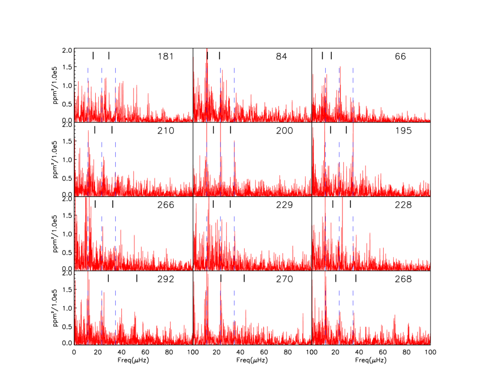
Figure 10: Power spectra for the 12 K giants with the lowest noise at high frequencies. The luminosity of the stars increases from the bottom to top panels and increases from left to right. The predicted location of the maximum $p$-mode power and the acoustic cutoff frequency (indicated by thick black lines) shift to lower frequencies for increasing luminosity. Frequencies at multiples of 11.57 $\mu$Hz (1 c/d) are indicated with vertical dashed lines.

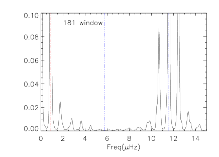
Figure 11: The autocorrelation of the spectral window for star #181. The vertical lines indicate peaks at 11.57, 5.84 and 0.81 $\mu$Hz (1, 0.5 and 0.07  c/d). Note that multiples of the 0.81 $\mu$Hz peak are present.

6.3 Subtracting 1 c/d aliases

We note that some of the observed excess peaks in the amplitude spectra are close to multiples of 1 c/d (11.57 $\mu$Hz) as indicated by the vertical dashed lines in Fig. 10. These peaks are likely due to residual effects of extinction. In some light curves a peak in the range $\nu$ = 0.8–0.9 $\mu$Hz was also detected as likely caused by the spectral window (cf. Sect. 6.2). Therefore, following the approach of Stello et al. (2006b ), we subtract these low frequency peaks if they are significant ($S/N>4$). We specify later in each case, whether we are using the raw or the cleaned spectra (cf. Sect. 7).

In Fig. 12 we show an example of the process for star #66. Daily alias variations are seen in the amplitude spectrum in panel (a). Panel (b) is the amplitude spectrum after subtracting two peaks indicated by the vertical tickmarks in panel (a). Panel (c) is the spectral window, which shows quite strong and complex sidelobes. The white noise level is $\simeq 60$ ppm and is calculated as the mean level in the frequency range 81–104$\,\mu$Hz.

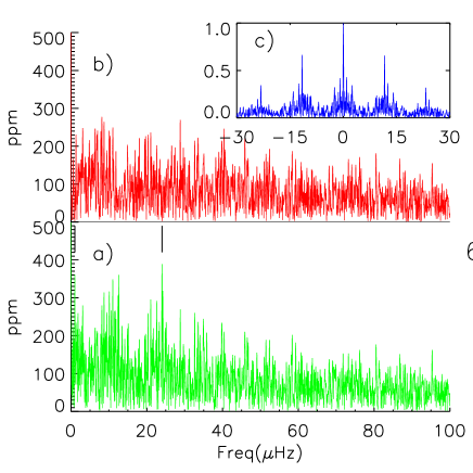
Figure 12: Amplitude spectra for star #66 which is the brightest, non-saturated star in the subsample chosen for a detailed analysis. Panel (a) is the raw spectrum with one low frequency peak and a peak close to 2 c/d (23.14 $\mu$Hz) marked. Panel (b) shows the amplitude spectrum after subtracting the two peaks marked with vertical lines in panel (a). Panel (c) shows the spectral window, which is seen to contain a complex substructure around each 1 c/d sidelobe.

6.4 Light curve simulations

To facilitate the interpretation of the observations in Sect. 7 we made simulations of the light curves. The time sampling and the noise properties are the same as for the observations and they include a known oscillation signal.

To mimic the noise we used the observed time series of two stars assuming that they resembled pure noise. The two stars (#66 and #292) are at either end of the luminosity range of the selected K giants. Both are among the K giant stars with the lowest noise in the amplitude spectra. The two stars show no clear evidence of power excess or a frequency separation that could arise from stellar oscillations.

We used different input amplitudes and life time of the modes using the simulation software described by De Ridder et al. (2006b ) and Stello et al. (stello04 (2004)).

7 A search for evidence of solar-like oscillations

Inspection of the K giant amplitude spectra in Fig. 10 reveals that the noise increases towards low frequencies, indicating that drift noise is present in the light curves. This will seriously hamper the interpretation of the signal below $\simeq 20$ $\mu$Hz. We see no clear evidence of excess power or the comb-like pattern expected for solar-like oscillations in any of the K giants. Although we find clear evidence for an increase in excess power towards low frequencies, it is not possible to disentangle drift noise and variation intrinsic to the K giant stars, eg. due to granulation or $p$-modes.

We have used two techniques to look for evidence of $p$-modes in the amplitude spectra:

• Autocorrelation of the amplitude spectra to search for the large separation (Sect. 7.1).

• A search for evidence of excess power in the expected frequency range (Sect. 7.2).

7.1 Autocorrelation

A clear proof of the presence of stellar oscillations would be a systematic behaviour of the observed frequency separations. The separation should increase with decreasing luminosity (cf. Eq. 5). In a few cases the autocorrelation shows a peak that could be indicative of the large separation. A prominent peak is seen in star #181 as shown in Fig. 13, where there is a peak at 2.75 $\mu$Hz (predicted to be at 2.55 $\mu$Hz). The highest peak at $\simeq$0.9 $\mu$Hz (vertical dashed line) is due to the window function (cf. Fig. 11) The autocorrelation was done on the raw spectrum. We find a few other stars with peaks in the autocorrelation spectrum that might come from the presence of a $p$-mode spectrum, but in the majority of cases we are not able to find a single prominent peak.

Figure 13: The autocorrelation of the raw power spectrum for the giant star #181. Vertical lines represent peaks in the window function. The peak at 2.75 $\mu$Hz could be the large separation, but might also be due to low frequency noise interacting with the window function.

We made several simulations of stars #66 and #292 with known input amplitude and lifetime as described in Sect. 6.4. We used two methods to search for the known large separations of the inserted modes. The first method was a simple autocorrelation technique and the second method cut up the spectrum in small pieces and added these pieces (like when an Echelle diagram is created) and then searches for peaks. The latter method is described by Christensen-Dalsgaard et al. (kepler (2007)). Both methods gave quite similar results. If the oscillations have a $Q$ value above 200, the correct large frequency separation $\Delta\nu_{0}$ is recovered in both stars for amplitudes down to 400 ppm.

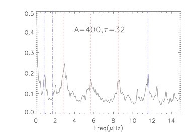
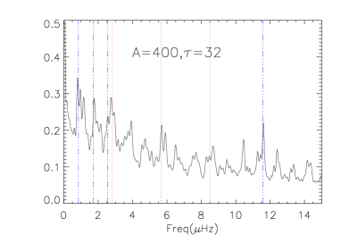
Figure 14: Autocorrelation of a simulation of star #292 including oscillations. In the top panel the spectrum of #292 was cleaned for multiples of 1 c/d before adding the simulated signal and in the bottom panel, the same procedure was followed as for the observed time series data. The red dotted lines correspond to multiples of the large separation in the simulated signal. The blue vertical lines indicate parasitic peaks from the window function at 0.85 and 11.57 $\mu$Hz (see Fig. 12).

In Fig. 14 we show the autocorrelation of the spectrum of star #292 including simulated oscillations with large separation 2.83 $\mu$Hz, amplitude $A$=400 ppm and lifetime $\tau$=32 d. We note that this lifetime is at least a factor two longer than expected. In the top panel the spectrum of #292 was cleaned for multiples of 1 c/d before adding the simulated signal. The autocorrelation clearly shows several peaks that correspond to the large separation present in the simulated signal (red dotted lines). The first dotted line indicates the large frequency separation present in the simulation, which repeats several times. The blue, dot-dash, vertical lines indicate parasitic peaks in the window function at 0.85 and 11.57 $\mu$Hz (see Fig. 11). In the bottom panel in Fig. 14 the procedure applied to the observed time series data was followed (see #181 in Fig. 13). In this case the input large separation is much harder to recover.

For the bright star (#66) for inserted amplitudes as low as $A=200$ ppm and large $Q$ values ($>$30) the large separation is recovered. However, if the lifetime is shorter than $\simeq$16 days ($Q<12$), we find that it is not possible to recover the input separation in any of the simulated series, even with amplitudes up to 800 ppm. Thus, our upper limits of 200–400 ppm only hold if the lifetime is greater than two weeks as predicted by Houdek & Gough (houdek02 (2002)) and Houdek (houdek06 (2006)), and not a few days as found by Stello et al. (2006a ).

7.2 A search for evidence of excess power

To search for excess power we followed the approach by Stello et al. (stello07 (2007)) used in their analysis of K giants in the open cluster M67. The K giant stars in M4 were put in three groups with luminosities around 60, 80, and 130 $\thinspace{\rm L}_{\odot}$ (faint, average or bright stars). For each group we calculated a mean raw amplitude spectrum. To demonstrate the effect of cleaning the spectra, we also produced a mean spectrum for the faint group of the cleaned spectra.

In Fig. 15 we show the mean spectra. The raw spectra for the three groups of stars are quite similar with prominent peaks near multiples of 1 c/d. This is unexpected and suggests that the power seen possibly is dominated by a noise component due to instrumental drift in the data.

Using the simulations described in Sect. 6.4 we probed our ability to identify the inserted oscillation signal. The black, solid spectrum in Fig. 15 is based on a mean of four time series of star #292 which includes simulations of $p$-modes using different lifetimes in the range 2–8 days and peak amplitudes of $A=400$ ppm per mode. This covers the range of expected lifetimes and averaging four simulations removes some of the stochastic features of the oscillations. This artificial spectrum is clearly above any of the observed mean spectra. Our conclusion is that excess power from $p$-modes with amplitudes $A>300$ ppm would show up clearly in our observed spectra.

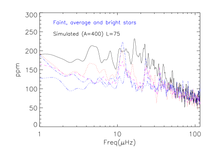
Figure 15: Average smoothed spectra for three groups of observed K giants with luminosity $L\simeq 60,80\leavevmode\nobreak\ {\rm and}\leavevmode\nobreak\ 130$ $\thinspace{\rm L}_{\odot}$. The faint group (raw and clean version) are the blue lines, the average group is plotted as the magenta line and the bright group is the red line. The bottom curve is the faint group after multiples of 1 c/d are removed. The black solid line is for a simulation of star #292 with peak oscillation amplitudes of $A=400$ ppm.

8 Comparison with 3D-hydrodynamical simulations of granulation

We have compared our results for the K giants with 3D hydrodynamical simulations of granulation by Svensson & Ludwig (g-simul (2005)). The effect of granulation is modelled by simulations of the convective motions in a box which is scaled to predict the effect expected to be observed when observing a spherical star. The result of Svensson & Ludwig (g-simul (2005)) indicate that K giants should have a low frequency component of granulation power similar to the noise levels achieved for some of the K giants in M4.

One of their simulations (Ludwig ludwig (2006); kindly provided by G. Ludwig) is shown as the dotted black curve in Fig. 16. The stellar parameters are $R/\hbox{$\thinspace{\rm R}_{\odot}$}=30.2,\log g=2.0,$ $T_{\rm eff}$ $=4560$ K, and metallicity [M/H] $=0.0$. This corresponds to a luminosity $L=385$ $\thinspace{\rm L}_{\odot}$, which is larger by roughly a factor two than the brightest K giants we have observed. The larger luminosity means that the simulated granulation has larger amplitudes and excess power at lower frequencies than for our brightest target.

A scaling of the solar power spectrum has been attempted by Kjeldsen & Bedding (in preparation) and by Stello et al. (stello07 (2007)). A white noise component with the same level as the star chosen for comparison (#66) is added to a scaled granulation signal and a scaled $p$-mode spectrum. The scaling is very crude, and a difference of a factor two from our K giants would not be surprising. The granulation spectrum is shown in a logarithmic plot of power density in Fig. 16.

The simulated spectrum (black dotted line) and the scaled spectrum (blue dashed line) both show a larger power density at low frequencies compared to the observations (red solid line). The peak of the observed spectrum coincides with the peak around 10 $\mu$Hz of the scaled spectrum, in which the power is due to the presence of oscillations. In the observed spectrum it is likely to be the 1 c/d alias.

The reason for the high power at low frequencies in the 3D simulations is because the luminosity of the model simulated is twice the luminosity of star #66. The amplitude of the power density should scale with $L^{2}$ and the frequency with $L^{-1}$, which will bring the 3D simulations closer to the other curves, but still above the observations. Svensson and Ludwig (g-simul (2005)) show that lowering the metal content in a 1 $\thinspace{\rm M}_{\odot}$ model makes the power density drop considerably. A change of metal content might remove the discrepancy between the observations and the 3D simulations of a giant. The 3D simulation (black dotted line) falls below the other curves at high frequencies since no white noise was included.

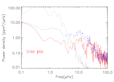
Figure 16: Power density for three cases: 1) the observed star #66 (red, solid line), 2) a scaled power spectrum including granulation, $p$-modes with $A=300$ppm and white noise as star #66 (blue, dashed line), 3) the simulation by Svensson and Ludwig (g-simul (2005)) (black, dotted line).

9 Conclusion and discussion

We have presented results for a three-site multi-colour photometric campaign on the globular cluster M4. We used data in the Johnson $BVR$ bands from 48 nights with a time baseline of 78 days.

We compared the precision of the photometry obtained from three different photometric packages. In the most crowded parts of the field we find the best results using a difference image analysis (Alard isis00 (2000)), while classical aperture photometry give better results in the semi-crowded regions. The best photometry is found for stars not affected by crowding, and in this case we achieve noise levels close to the theoretical noise limit.

The main goal of the campaign was to detect solar-like oscillations in the rich population of K giant stars in M4. However, we are not able to claim an unambiguous detection and we summarize our conclusions here:

• We detect no individual peaks with $S/N>4.0$.

• We find no significant large frequency separation from the autocorrelation of the amplitude spectrum.

• We divided the stars with the best photometry in three groups and computed the average power spectra. From a comparison of the spectra with realistic simulations of granulation and an assumed comb-like distribution of $p$-modes, we can exclude that power is present from $p$-modes with peak amplitudes above 300 ppm whatever the damping time. This upper limit is in accordance with the $(L/M)^{0.7}$ scaling suggested by Samadi et al. (samadi (2006)) which predicts amplitudes below 300 ppm for the most luminous stars, but far below the scaling law $L/M$ from Kjeldsen & Bedding (kandb (1995)).

• In all K giants the amplitude increases towards low frequencies. This would be consistent with granulation, but we find that the observed increase does not vary with stellar luminosity. Thus we cannot differentiate between drift noise in the data and the expected granulation signal.

• We have compared the observations with a 3D-hydrodynamical simulation for solar metallicity. The observed power density at low frequencies is much lower than the simulations of granulations predict. In their 3D simulations Svensson & Ludwig g-simul (2005) found that the granulation power is substantially smaller for lower metallicity (M4 has [Fe/H] $=-1.2$). This could explain that our data, even for the brightest star, falls considerably below the simulations (Fig. 16).

Our negative results support the recent evidence for short lifetimes in giant stars (Stello et al. 2006a ) but contradict the theoretical predictions by Houdek & Gough (houdek02 (2002)).

For the population II star $\nu$ Indi, which has a low luminosity (6 $\thinspace{\rm L}_{\odot}$), $p$-modes have been detected (Bedding et al. bedding06 (2006), Carrier et al. carrier07 (2007)). However, we cannot tell whether the stochastic driving still works in population II stars around $L=100$ $\thinspace{\rm L}_{\odot}$, although we can say it cannot be very efficient and certainly not exceeding amplitudes following the $(L/M)^{0.7}$ scaling relation suggested by Samadi et al. (samadi (2006)).

This is contrary to the conclusion by Stello et al. (stello07 (2007)) for the K giants in M67, who found indications of $p$-mode power in stars at lower luminosities (10–20 $\thinspace{\rm L}_{\odot}$). They find better agreement between observations and predictions if the amplitudes scale as $L/M$. Their noise level at low frequencies do not permit any statement for stars at luminosities similar to the stars investigated in M4. It remains an open question, whether the stochastic driving still works without being destroyed by convective or radiative processes in population II K giants.

Based on the results obtained from large multisite campaigns on M67 and M4, it seems difficult to get conclusive positive results about the stochastic oscillations and the granulation from ground-based photometry. Improvements can be made, but extinction and other atmospheric effects will always be a limiting factor and especially so at the time scales of the K giants. It is also difficult to get a clean window function due to changing weather patterns for campaigns lasting several weeks, which is unfortunately needed to study solar-like oscillations in K giant stars.

9.1 Directions for the future

If a new campaign is organized we recommend to use a single filter, as colour information is not likely to be of a quality that can lead to mode identification. We found no use for the differences between the filters. We recommend that the $V$ filter is used in the future: the $B$ filter observations show strong colour-dependent extinction and the amplitudes will be very low in $R$.

From the ground one would do better by organizing a longterm radial velocity campaign. One immediate advantage is that the noise from granulation is 10 times lower in velocity (Grundahl et al. song (2007), their Fig. 1). One could observe several K giants during the night since the time scale of the oscillations is several hours. A dedicated network providing good time coverage would be needed in order to obtain a clean window function. The proposed SONG network (Grundahl, et al. song (2007)) is an example of such a programme.

For fast rotating stars where the broad spectral lines prevent precise velocity results to be obtained, observations of solar-like oscillations can be made with photometry from space. This has resulted in the measurements of variability in population I G giants by the WIRE satellite (Buzasi, Bedding & Retter wire1 (2003)), and $p$ modes in $\eta$ Boo with the MOST satellite (Guenther et al. most (2005)).

Giants are also among the targets for the new photometric satellite missions like the CoRoT mission (Baglin, Michel & Auvergne corot (2006)) and the future Kepler mission (Christensen-Dalsgaard et al. kepler (2007)). The CoRoT mission observes the same part of the sky for up to 150 days while the Kepler mission will cover many more targets for up to six years.

- (1) Alard, C. 2000, A&AS, 144, 363
- (2) Alard, C., & Lupton, R. H. 1998, ApJ, 503, 325
- (3) Alonso, A., Arribas, L. & Martinez-Roger, C. 1999, 140, 261
- (4) Baglin, A., Michel, E., Auvergne, M. et al. 2006, Proc. of SOHO 18/GONG 2006/HELAS I, Beyond the spherical Sun (ESA SP-624), Eds. K. Fletcher & M. Thompson, CDROM, p.34.1
- (5) Barban, C., De Ridder, J., Mazumdar, A. et al. 2004, in Proceedings of the SOHO 14 / GONG 2004 Workshop (ESA SP-559), ed. D. Danesy, 113
- (6) Bedding, T. R. et al. 2006, ApJ, 647, 558
- (7) Bedding, T. R. et al. 2007, ApJ, accepted, (Astro-ph/0702747)
- (8) Bruntt, H. 2003, Ph.D. Thesis, University of Aarhus (Denmark)
- (9) Bruntt, H., Grundahl, F., Tingley, B., Frandsen, S., Stetson, P. B., & Thomsen, B. 2003, A&A, 410, 323
- (10) Bruntt et al., 2007, MNRAS, in press
- (11) Buzasi, D., Bedding, T., & Retter, A. 2003, Solar and Solar-Like Oscillations: Insights and Challenges for the Sun and Stars, 25th meeting of the IAU, Joint Discussion 12, 18 July 2003, Sydney, Australia, 12
- (12) Carrier, F., et al. 2007, ArXiv e-prints, 706, arXiv:0706.0795
- (13) Christensen-Dalsgaard, J. et al. 2007, astro-ph/0701323
- (14) Collet, R., Asplund, M. & Trampedach, R. 2007, astro-ph/0703652
- (15) De Ridder, J., Barban, C., Carrier, F., Mazumdar, A., Eggenberger, P., Aerts, C., Deruyter, S., & Vanautgaerden, J. 2006a, A&A, 448, 689
- (16) De Ridder, J., Arentoft, T. & Kjeldsen, H. 2006b, MNRAS, 365, 595
- (17) Döllinger, M. P., Pasquini, L., Hatzes, A. P. et al. 2005, The ESO Messenger, 122, 39
- (18) Edmonds, P. D. & Gilliland, R. L. 1996, ApJ, 464, L157
- (19) Frandsen, S., Carrier, F., Aerts, C. et al. 2002, A&A, 394, L5
- (20) Gilliland, R. L., Brown, T. M. 1992, PASP, 104, 582
- (21) Gilliland, R. L., Brown, T. M., Kjeldsen, H. et al. 1993, AJ, 106, 2441
- (22) Guenther, D. B., Kallinger, T., Reegen, P. et al. 2005, ApJ, 635, 547
- (23) Grundahl, F., Kjeldsen, H., Christensen-Dalsgaard et al. 2007 Comm. in Asteroseismology, accepted
- (24) Handler, G. 2003, Baltic Astronomy, 12, 253
- (25) Houdek, G., Gough, D. O. 2002, MNRAS, 336, L65
- (26) Houdek, G. 2006, preprint astro-ph/0612024
- (27) Ivans, I. I. et al. 1999, AJ 118, 1273
- (28) Jiménez, A., Roca Cortés, T., Severino, G. & Marmolino, C. 1999, ApJ, 525, 1042
- (29) Kjeldsen, H., & Frandsen, S. 1992, PASP, 104, 413
- (30) Kjeldsen, H. & Bedding, T. R. 1995, A&A, 293, 87
- (31) Kjeldsen, H., & Bedding, T. R. 2004, ESA SP-559: SOHO 14 Helio- and Asteroseismology: Towards a Golden Future, 14, 101
- (32) Kjeldsen, H., Bedding, T. R., Butler, P. R. et al. 2005, ApJ, 635, 1281
- (33) Kopacki G., 2000, A&A, 358, 547
- (34) Kopacki G. & Frandsen, S. 2007 Comm. in Asteroseismology, accepted
- (35) Ludwig, H. G., 2006, A&A, 445, 661
- (36) Samadi, R., Georgobiani, D., Trampedach, R., Goupil, M.J. et al. A 2006, astro-ph 0611762
- (37) Sperl, M. 1998, Comm. in Asteroseismology, 111, 1
- (38) Stello, D., Kjeldsen, H., Bedding, T. R., de Ridder, J., Aerts, C., Carrier, F., & Frandsen, S. 2004, Sol. Phys., 220, 207
- (39) Stello, D., Kjeldsen, H., Bedding, T. R. & Buzasi, D. 2006a, A&A, 448, 709
- (40) Stello, D. et al. 2006b, MNRAS, 373, 1141
- (41) Stello, D., Kjeldsen, H., Bedding, T. R., Buzasi, D. 2006c, MmSAI, 77, 406
- (42) Stello, D. et al. 2007, 377, 584
- (43) Stetson, P. B. 1987, PASP, 99, 191
- (44) Stetson, P. B. 1990, PASP, 102, 932
- (45) Stetson, P. B. 1994, PASP, 106, 250
- (46) Stetson, P. B. 2007, http://www.physics.mcmaster.ca/Globular.html
- (47) Svensson, F. & Ludwig, H.-G. 2005, in Proc. 13th Cambridge Workshop on Cool Stars, Stellar Systems and the Sun (ESA SP-560), Eds. F. Favata, G. Hussain & B. Battrick, 979