The empirical metallicity dependence of the mass-loss rate
of O- and early B-type stars

We present a comprehensive study of the observational dependence of the mass-loss rate in stationary stellar winds of hot massive stars on the metal content of their atmospheres. The metal content of stars in the Magellanic Clouds is discussed, and a critical assessment is given of state-of-the-art mass-loss determinations of OB stars in these two satellite systems and the Milky-Way. Assuming a power-law dependence of mass loss on metal content, $\dot{M}\propto Z^{m}$, and adopting a theoretical relation between the terminal flow velocity and metal content, $v_{\infty}\propto Z^{0.13}$ (Leitherer et al. 1992), we find $m=0.83\pm 0.16$ for non-clumped outflows from an analysis of the wind momentum luminosity relation (WLR) for stars more luminous than $10^{5.2}L_{\odot}$. Within the errors, this result is in agreement with the prediction $m=0.69\pm 0.10$ by Vink et al. (2001). Absolute empirical values for the mass loss, based on H$\alpha$ and ultraviolet (UV) wind lines, are found to be a factor of two higher than predictions in this high luminosity regime. If this difference is attributed to inhomogeneities in the wind, and this clumping does not impact the predictions, this would imply that luminous O and early-B stars have clumping factors in their H$\alpha$ and UV line forming regions of about a factor of four. For lower luminosity stars, the winds are so weak that their strengths can generally no longer be derived from optical spectral lines (essentially H$\alpha$) and one must currently rely on the analysis of UV lines. We confirm that in this low-luminosity domain the observed Galactic WLR is found to be much steeper than expected from theory (although the specific sample is rather small), leading to a discrepancy between UV mass-loss rates and the predictions by a factor 100 at luminosities of $L\sim 10^{4.75}L_{\odot}$, the origin of which is unknown. We emphasize that even if the current mass-loss rates of hot luminous stars would turn out to be overestimated as a result of wind clumping, but the degree of clumping would be rather independent of metallicity, the scalings derived in this study are expected to remain correct.

1 Introduction

Understanding the properties and evolution of massive stars in low metallicity environments is of fundamental importance in astrophysics. This is amply illustrated by referring to the anticipated role of massive stars in the early universe, where they are thought to be responsible for its re-ionization (e.g. Haehnelt et al., 2001; Wyithe & Loeb, 2003), galaxy formation, and chemical evolution of young galaxies and of the intra-galaxy medium. Strong indications of gamma-ray bursts occurring primarily at low metallicity (e.g. Gorosabel et al., 2005) and massive stars being progenitors (e.g. Hjorth et al., 2003), adds to the point. To a large extent, the evolution of massive stars is controlled by the effects of mass loss, therefore mass loss has a direct and/or indirect impact on all the phenomena mentioned above. This makes a quantitative handle on the dependence of mass loss on the metal content of the environment out of which these early stars form so vital. Obviously this argument also applies to massive stars in the local universe.

In the last decade the development of realistic stellar atmosphere models has allowed accurate determination of the wind parameters of a sizeable sample of early-type Galactic stars (e.g. Puls et al., 1996; Herrero et al., 2002; Repolust et al., 2004; Crowther et al., 2006). This, in turn, has allowed us to test our understanding of aspects of stellar wind hydrodynamics, including its driving mechanism, to an unprecedented level. During this period new instrumentation developements on large telescopes have resulted in significant numbers of extragalactic stars being spectroscopically studied. Examples of extensive surveys are those of Massey et al. (2004, 2005) and of Evans et al. (2005), although there are many others and the relevant ones will be discussed later. The latter program is the VLT-FLAMES Survey of Massive Stars, in which close to 100 O- and early B-type stars were observed in the Magellanic Clouds. The inclusion of line blocking/blanketing in the modeling of hot star atmospheres (e.g. Hubeny & Lanz, 1995; Hillier & Miller, 1998) allows for a consistent description of the effects from vast numbers of overlapping metal lines, particularly regarding a detailed treatment of the effects of chemical composition, and has paved the way for a robust quantitative comparison of the wind strengths of hot massive stars in different metallicity environments. The most recent step forward in the modeling technique has been the development of an automated fitting method, opening up a means to analyse large samples in a homogeneous way (Mokiem et al., 2005).

This paper provides a critical assessment of the current standing of mass-loss determinations in the Galaxy and the Large and Small Magellanic Clouds, and is specifically aimed at establishing the dependence of mass loss on the chemical abundance pattern, notably metal content $Z$. The Small Magellanic Cloud (SMC) with $Z$ at about 1/5th of the Galactic value is the lowest metallicity we can so far probe in reasonable detail. The Large Magellanic Cloud (LMC) with approximately half the metal content of the Galaxy provides an intermediate environment.

The only possibility, in the forseeable future, of studying stars in environments with significantly lower metallicity than the SMC is the massive stellar populations of the Local Group dwarfs GR8, Sextans A and Leo A. These three galaxies have metallicities betweem 0.1 and 0.05 Z_⊙, but their low starformation rates and distances of around 1-2 Mpc makes studies of large numbers of young massive stars extremely difficult. Given this difficulty of establishing the dependence of mass-loss rates upon metallicity below 1/5 Z_⊙, we must rely on predictions to access this interesting part of parameter space. Although we do not deal with the theory of wind driving mechanism, we will compare predicted and observed wind strengths to establish successes and failures of the theory such that we may identify aspects of the $\dot{M}(Z)$ problem that require further study, and regimes in parameter space that seem sufficiently under control to allow us to venture out to lower metallicity regimes and the early universe (see also Vink & de Koter, 2005).

In Sect. 2 we briefly review the mass-loss mechanism of early-type stars. The present day chemical composition of the Galaxy and Magellanic Clouds is discussed in Sect. 3. Sections 4 and 5 describe the methodology used to determine mass-loss rates and how to compare these for different chemical environments. The observed mass-loss relations are presented in Sect. 6. On these relations the global metallicity dependence of $\dot{M}$ is determined in Sect. 7. Finally, in Sect. 8 we discuss the observed mass-loss relations in terms of the so-called weak wind problem and wind clumping, and end with concluding remarks.

2 The mass-loss mechanism of early-type stars

We briefly review those aspects of the wind driving mechanism of massive early-type stars that are relevant in the context of establishing an empirical relation between mass loss and chemical composition. For a more in-depth treatment of the physics of mass loss, see e.g. Kudritzki & Puls (2000) and Vink et al. (2001). The basic mechanism driving the winds of hot massive stars is the transfer of momentum from photons to the atmospheric gas by line interactions. The driving mechanism implies that the properties of the stellar wind will depend on the number of photons per second streaming through the photospheric layers (reflecting the stellar luminosity), and on the number and ability of lines being available – in particular at wavelengths around the photospheric flux maximum – to absorb or scatter these photons.

Table 1: Overview of the ions that dominate the line driving in early-type stars – for solar metallicity with $L_{\star}=10^{5}$ $L_{\odot}$. See Sect. 2 for a discussion.

	$T_{\rm eff}$= 20 kK	$T_{\rm eff}$= 25 kK	$T_{\rm eff}$= 30 kK	$T_{\rm eff}$= 40 kK
Atom	Contr. %	Contr. %	Contr. %	Contr. %
H	19.53	14.84	12.82	14.11
He	0.01	0.03	0.05	0.05
C	2.61	12.28	14.43	24.03
N	0.49	1.09	1.76	7.19
O	0.65	0.14	1.87	4.64
Mg	2.07	0.46	3.08	–
Al	2.17	3.21	12.61	–
Si	7.95	10.01	20.34	13.16
P	6.56	9.46	0.93	1.13
S	4.51	6.52	4.55	16.51
Cl	0.30	1.57	1.05	0.91
Ar	0.11	0.24	0.33	1.87
Cr	2.36	1.98	0.78	0.48
Mn	1.10	0.92	1.07	0.34
Fe	39.00	32.29	23.07	10.51
Ni	6.40	4.03	0.65	2.40
Rest	4.18	0.93	0.61	2.67

The dependence of the wind driving on the number of lines present suggests that mass loss is a function of elemental abundance. Whether this is indeed the case formally depends on the nature of the driving lines. In the hypothetical case that one would be in a regime of abundances for which all lines effectively contributing to the line force are optically thick, mass loss would not be a function of elemental abundance. This regime is not encountered in even the most metal rich environments known (Vink et al., 2001). In reality, it is found that the lines driving the wind are a mixture of optically thin and optically thick lines. Representing the distribution of line strengths by a power law, one predicts, for Galactic O stars, a ratio of the line acceleration from optically thick lines to the total line acceleration of $\alpha\sim 2/3$ (see Puls et al., 2000), where an even larger contribution by optically thick lines would increase this value (and vice versa). This ensures a dependence of mass loss on elemental abundance.

Which elements dominate the line force? The answer depends on the effective temperature of the star. (More precisely: on the radiation and electron temperature in the wind acceleration regime; see also Vink et al., 1999; Puls et al., 2000). Although hydrogen and helium are by far the most abundant elements, their impact on the wind driving is modest. Decisive for whether or not a species is a significant contributor to the line driving is the product: abundance $\times$ ionisation fraction $\times$ number of effective lines. Very roughly, the elemental abundance times the ionisation fraction of hydrogen and helium are similar to that of metals that are in the dominant stage of ionisation. It is therefore the number of driving lines that is decisive. As H and He – due to their simple atomic structure – have only few lines that can effectively contribute to the line force, it is relatively abundant complex atoms that are the main contributors.

We estimate the relative contributions of the different elements by the use of a Monte Carlo method (Abbott & Lucy, 1985; de Koter et al., 1997; Vink et al., 1999) that calculates the total momentum transfer from the radiation field to the outflowing gas particles. Although the relative contribution to the line force is depth-dependent (see below), here we simply register the atomic number of the elements with which the photons interact somewhere in the wind, and we present the results in Tab. 1. For a late-O dwarf of solar composition, CNO accounts for some 15 percent; iron contributes some 25 percent. Other iron-group elements (for instance Cr, Mn, Co, Ni) add a few percent. $\alpha$-elements, such as Ne, Mg, Si, S, Ar, and Ca account for about 30 %, with Si being the main contributor with $\sim$ 20 %. We mention a decomposition of the line force in terms of iron group and $\alpha$ elements as their nucleosynthetic origin is different. The former are mostly produced in thermonuclear Type Ia supernovae, the latter predominantly in core-collapse supernovae of types II and Ib/c. Beware that due to their different electronic structure specific groups of elements have a different line-strength statistics, and dominate the line acceleration at different depths: iron group elements have a somewhat larger influence on the mass-loss rate, whereas lighter ions dominate the acceleration in the outer wind, thus controlling the terminal velocity (cf. Vink et al. 1999; Puls et al. 2000). These more subtle effects are not reflected in the statistics provided in Table 1.

Mixing of CNO-cycled material to the surface during the supergiant phase may affect the relative abundances of these three elements. However, in terms of their contribution to the line force not much will change when this happens, as these three elements have more or less equal numbers of effective driving lines near the photospheric flux maximum and the C+N+O abundance remains unaffected by the CNO-cycle (Vink & de Koter, 2002).

Accounting for the fact that we are interested in the gross dependence of wind parameters on metallicity, and particularly in the product of mass-loss rate and terminal velocity (see below), we conclude that a straight mean of C+N+O, $\alpha$-elements, and iron-group elements is an appropriate abundance value to use as a $Z$ measure for O stars. For stars of spectral type B and A the contribution of iron increases to up to 50 percent.

3 Metallicity determinations of early-type stars

Having identified the elements that dominate the line force, we now address the present-day chemical composition of hot massive stars in the Galaxy and the Magellanic Clouds.

Spectroscopy of H ii regions and supernova remnants have been used to probe the gas phase composition of the Magellanic Clouds (for reviews see for instance Pagel et al., 1978; Dufour, 1990; Russell & Dopita, 1990; Garnett, 1999). The results derived from these studies do not necessarily represent the initial chemical composition of the stars in these environments because of fractionation of some elements from the gas phase onto solid state particles (or “dust”). Also, emission line studies may be affected by spatial inhomogeneities in the nebula. Therefore, to obtain the appropriate chemical composition of the winds we are studying it would be pertinent to determine the photospheric abundances of the massive stellar populations in the Clouds. As the comparison between theoretical and observed wind strength is usually not done on an individual basis (but see de Koter et al., 1997) it is relevant to specify how the observed metal abundance $Z$ – so far the abundance input parameter for mass-loss predictions – is derived. If $Z$ is derived from CNO abundances in either evolved or rapidly rotating objects one should be careful. In supergiants and even giants (Korn et al., 2000; Lennon et al., 2003) rotational mixing and ejection of the outermost envelope by mass loss may bring CNO equilibrium material to the surface. In stars rotating at about half of break-up at the surface or more, abundance alterations due to rotational mixing may already occur very early on in the stars evolution (Yoon & Langer, 2005).

The optical spectra of O stars show few spectral lines of heavy elements. B stars are relatively rich in absorption features due to C, N, O, Mg, Al, Si, S, and Fe providing a sound basis for establishing the metallicity, although we note that the Fe lines are intrinsically quite weak (especially so in the SMC; Rolleston et al., 2003). The advantage of B and later-type dwarf and giant stars is also that they may be analysed accurately using non-LTE line-blanketed hydrostatic atmospheres, without winds.

Table 2: Present-day chemical composition of the LMC and SMC from B-type stars. The values are taken from Hunter et al. (2007) and Trundle et al. (2007) apart from Al and S which are LTE results from Rolleston et al. (2002, 2003). For comparison the solar abundances of Asplund et al. (2005) also given.

Element	Solar	LMC		SMC
		$12+\log X/{\rm H}$	$\Delta[X/{\rm H}]$	$12+\log X/{\rm H}$	$\Delta[X/{\rm H}]$
C	8.39	7.73	$-$0.66	7.37	$-$1.02
N	7.78	6.88	$-$0.90	6.50	$-$1.28
O	8.66	8.35	$-$0.31	7.98	$-$0.68
Mg	7.53	7.06	$-$0.47	6.72	$-$0.81
Al	6.37	…	…	5.43	$-$0.72
Si	7.51	7.19	$-$0.32	6.79	$-$0.72
S	7.14	…	…	6.44	$-$0.42
Fe	7.45	7.23	$-$0.29	6.93	$-$0.57

A major goal of the VLT-FLAMES survey of massive stars (Evans et al., 2005) was to observe a large number of such B-type stars in the same vicinity as the O-stars to determine their photospheric abundances. Hunter et al. (2007) and Trundle et al. (2007) have presented the chemical compositions of 34 and 53 B-type stars in the SMC and LMC respectively. These are the narrow lined stars from the FLAMES survey, with the highest signal-to-noise spectra, analysed with the line-blanketed non-LTE code tlusty. These authors determined the best estimates for the chemical composition of the Clouds from a comparison of results from stellar and nebular work, and we summarise and extend their results in Table 2. The non-LTE absolute abundances for C, N, O, Mg, and Si are quoted, along with the simple difference between these absolute values and the current standard solar abundances of Asplund et al. (2005). However detailed non-LTE model atoms for use in calculating line profiles for Al, S and Fe in tlusty are required to allow reliable line abundances to be calculated consistently in non-LTE. The results for Fe are taken from Trundle et al. (2007) in which a non-LTE atmosphere and LTE line formation calculations were used. The results for Al and S are taken from the LTE B-star analysis of Rolleston et al. (2003) and Rolleston et al. (2002). Because we are less certain of the validity of the absolute values of the LTE results, we quote the differential abundances from these papers which were determined from analysing Galactic B-stars with identical atmospheric parameters. We should also note that the Rolleston et al. (2003) abundances come from the analysis of a single star AV304, and the LMC results are from 5 stars with spectra of modest signal-to-noise.

The SMC abundance of the $\alpha$ elements (O, Mg, Si) has a mean relative to solar of $\Delta[\alpha/{\rm H}]=-0.7\pm 0.1$ dex. The differential LTE result of Al is in good agreement with this value, although the one S abundance from the star AV304 is somewhat higher. The Fe abundance is $\Delta[{\rm Fe}/{\rm H}]=-0.57\pm 0.16$ dex, which, within the uncertainties, is in agreement with the $\alpha$ elements. The SMC Fe abundance has also been determined through studies of AFGK supergiants, which have more and stronger metal lines in their spectra and for which non-LTE effects are less important. They tend to show very good agreement at $\Delta[{\rm Fe}/{\rm H}]=-0.60\pm 0.1$ dex (Venn, 1999). Differences in modelling techniques/codes, diagnostic lines, and atomic data will clearly lead to systematic differences between the sets of results. The discrepancies between different analyses are becoming smaller, but have not completely been resolved and progress is required in the model atmosphere and line formation codes, particularly with regard to atomic data for S, Al and Fe for B-star analysis. We adopt $\Delta[Z/{\rm H}]\sim-0.7\pm 0.1$ for the SMC, but will discuss the effects of a potentially different metallicity later (see Sect. 7.2).

The abundance of the $\alpha$ elements in the LMC relative to solar from Hunter et al. (2007) and Trundle et al. (2007) is $\Delta[\alpha/{\rm H}]=-0.36\pm 0.1$ dex. An extensive comparison of abundance determinations in the LMC was compiled by Rolleston et al. (2002). Reasonable agreement is found between six independent studies of the overall metallicity of the LMC – irrespective of the class of object used to trace the chemical composition or the spatial location of the investigated stars. The mean metallicity, based on O and Si, is ($\Delta[{\rm O}/{\rm H}]+\Delta[{\rm Si}/{\rm H})/2=-0.30\pm 0.08$ dex. Some previous analyses using OB stars seem to indicate that iron is less deficient than the $\alpha$-elements. Rolleston et al. (2002) report an $\alpha$ to iron ratio $\Delta[\alpha/{\rm Fe}]\sim-0.14$ dex for main sequence OB stars, consistent with that obtained for evolved B-stars (Korn et al., 2000). However Trundle et al. (2007) determine a mean differential Fe abundance of $-0.29\pm 0.15$ for 13 stars of their sample in NGC2004, in good agreement with the depletions of O, Mg and Si. Studies using F supergiants and Cepheids, however, report iron abundances representative of the mean metallicity (Hill et al., 1995; Luck et al., 1998). In this study, we adopt $\Delta[Z/{\rm H}]\sim-0.3\pm 0.1$ for the LMC.

We note that for C and N the values in Hunter et al. (2007) are the best estimates of the baseline abundances in the Clouds. I.e. they are estimates of the C and N when the stars are born and before any rotational mixing has caused the photospheric abundances to change. It has been clear for some time that C and N are significantly underabundant in the Clouds in comparison to the heavier elements. This may have an effect on the wind strengths of the hottest stars where CNO (mainly C) is a significant contributor to the line force. (see Table 1).

4 Mass-loss determinations of early-type stars

During recent years, three basic diagnostics to derive the mass-loss rate of early-type stars have been employed. These are: (a) infrared, millimetre and radio excess due to free-free processes; (b) ultraviolet resonance lines, and (c) optical lines, notably H$\alpha$, but for the hottest stars also He ii $\lambda 4686$. For a didactic explanation of the way in which $\dot{M}$ can be derived from these diagnostics, see Lamers & Cassinelli (1999). In the context of the dependence of mass loss on metal content, millimetre and radio excess emission in early-type stars is (at this moment) impracticable as the flux levels are weak and can only be measured for not too distant Galactic stars (up to a few kiloparsec), i.e. the method can not be applied to Magellanic Cloud stars.

UV resonance lines of relatively abundant elements such as C, N, O and Si are the most sensitive probes of mass loss, allowing detection of rates as low as $\sim 10^{-9}\,M_{\odot}{\rm yr}^{-1}$. The lines typically saturate at about $\sim 10^{-7}$ $M_{\odot}{\rm yr}^{-1}$, therefore for strong winds they only provide lower limits to $\dot{M}$. Because of the ease with which the lines saturate, unsaturated lines often relate to minor ionisation stages (and/or, obviously, to weak winds). The ionisation of these trace ions may depend rather critically on the treatment of line-blanketing, clumping, and shocks. Over the past decade, line-blanketing has been incorporated into model atmosphere codes for hot stars with winds. In a detailed comparison of three of these codes, Puls et al. (2005) conclude that the flux levels at $\lambda\gtrsim 400$ Å agree very well. Below 400 Å, discrepancies are found, implying that the population of species such as N iv, C iv, and O vi should be taken with care, as should the mass-loss rates derived using these ions. One of the most important current challenges in model atmospheres treating outflows is to implement the direct and indirect effects of the line-driven instability (see e.g. Lucy & Solomon, 1970; Owocki, 1994, and references therein). This instability causes the formation of small scale density and velocity gradients in the wind flow, creating “clumps” of gas and shocks leading to X-ray emission and enhanced EUV-flux. We will discuss clumping in more detail in Sect. 8.2. Shocks may also impact on the ionisation of the species mentioned above. This presents a second reason for being cautious with the $\dot{M}$ values derived from UV resonance lines of which the ionisation is affected by EUV and/or X-ray photons. A third reason to be cautious is that the abundances of C, N, and O may be affected by the surfacing of nuclear processed material (see Sect. 3).

The third approach to derive the rate of mass loss is by fitting the H$\alpha$ profile, and, for stars of roughly spectral type O5 or earlier, He ii $\lambda 4686$. The advantages of fitting these lines compared to ultraviolet resonance lines are that i) the abundance determination is robust (for the most detailed approach, see Mokiem et al., 2005, 2006); ii) at least for hydrogen, the ionisation balance is well known, i.e. it is not affected by shock processes (which might still be a problem for helium). On the down side however, the H$\alpha$ diagnostic is not as sensitive as are the UV lines. For OB stars, only for mass-loss rates in excess of $\sim 10^{-7}$ $M_{\odot}{\rm yr}^{-1}$ can the contribution of wind emission to the H$\alpha$ photospheric line be used to determine $\dot{M}$. Even more, at such low wind densities the uncertainty about the velocity law (which cannot be constrained if the wind emission inside H$\alpha$ is low) introduces an additional ambiguity, which increases the errors in the derived mass-loss rate considerably, up to factors of two to three (e.g., Puls et al. 1996).

This poses a challenge: the H$\alpha$ and UV resonance line diagnostics have only a small mass-loss regime in common in which both techniques can be applied simultaneously. This is unfortunate in view of resolving the weak wind problem (see Sect. 8.1), although there may be alternative wind diagnostics. First, the Br$\alpha$ line at 4.05 $\mu$m is intrinsically stronger than H$\alpha$ and could push the sensitivity of the hydrogen line $\dot{M}$-diagnostic by possibly a factor two to three (Schaerer et al., 1996; Lenorzer et al., 2004; Repolust et al., 2005) or even more (as resulting from test calculations by JP and FN), providing sufficient overlap to derive $\dot{M}$ from both methods for a reasonable number of stars. Second there is a P v resonance doublet at $\lambda\lambda$1118,1128 Å. The abundance of phosphorus is about a factor of $10^{2}-10^{3}$ less than that of C, N, O, and Si. As a result of this the line does not saturate as easily. Consequently, it can be applied to stars with $\dot{M}$ in excess of $10^{-7}$ $M_{\odot}{\rm yr}^{-1}$ (see e.g. Crowther et al., 2002; Hillier et al., 2003). Moreover, for a range of O subtypes P v is expected to be the dominant ionisation stage (for recent results, see Puls et al. 2007), making it less susceptible to shocks. Access to the far-ultraviolet region of the spectrum is provided by, for instance, the Far Ultraviolet Spectroscopic Explorer. Analysis of spectra obtained with this instrument strongly points to discrepant P v and H$\alpha$ based mass-loss rates, suggestive of clumped winds (Massa et al., 2003; Fullerton et al., 2006).

5 Comparing $\dot{M}$ in different environments

How should we compare the mass-loss rates of OB stars in different galaxies? The most straightforward way of doing this would be to consider two stars with almost identical parameters – one in each galaxy – and directly compare their $\dot{M}$ values. There are two arguments against such an approach. The first one is of a practicable nature. The number of O and early-B stars studied in the Galaxy and the Magellanic Clouds is so far too limited to identify a significant number of stars with “identical” luminosity, temperature, mass, and to a lesser extent rotational and terminal wind velocity. The impact of stellar rotation on mass loss appears important only for stars close to the $\Omega$-$\Gamma$ limit (e.g. Maeder & Meynet 2000 and Lamers 2004, and, e.g., van Boekel et al. 2003 and Smith et al. 2003 for the extreme case of $\eta$ Carinae), therefore, for relatively “normal” early-type stars one may consider it less critical. Terminal velocity differences due to metallicity effects are found to be minor, both from observational (e.g. Evans et al., 2004b) and theoretical (e.g. Puls et al., 2000; Krtička, 2006) considerations.

Even if for a few cases one could perform such a direct comparison, it would still not be an appealing approach, as the $\dot{M}(Z)$ relation may not necessarily be universal for all stellar parameters, and the result might not be applicable to all early-type stars. Therefore, the second reason against an object-to-object comparison is that it may ignore potential physical arguments that would allow the entire parameter space of hot massive stars be used to establish the mass loss-metallicity relation, and that would add predictive power to the derived $\dot{M}(Z)$.

Indeed the radiation-driven wind theory makes such predictions, and a powerful way to proceed is through the use of the so-called modified wind momentum – luminosity relation, (WLR; e.g. Kudritzki et al., 1995; Kudritzki & Puls, 2000)

$$\log\mbox{$D_{\rm mom}$}\equiv\log\left(\dot{M}v_{\infty}\sqrt{R}\right)\simeq x\log(L_{\star}/L_{\odot})+\log\mathit{D}_{\circ}\leavevmode\nobreak\ .$$ (1)

In this relation the slope $x$ and the constant $\mathit{D}_{\circ}$ are expected to vary as a function of spectral type and metal content (Kudritzki et al., 1999; Vink et al., 2000; Puls et al., 2000). This equation expresses that the mechanical momentum of the stellar wind flow is primarily a function of photon momentum. It is perhaps surprising that the stellar mass does not feature in this dependence. The reason is that $\log\mathit{D}_{\circ}$ contains a term $\propto(3/2-x)\log M$, which (almost) vanishes since $x$ happens to be $\sim 3/2$ for O-stars and early B-supergiants (Puls et al., 2000). The uniqueness of the modified wind momentum relation has been confirmed by independent investigations (e.g Vink et al., 2000; Puls et al., 2003). In Tab. 3 coefficients for the WLR as predicted by Vink et al. (2000, 2001) are given for the Galactic, LMC and SMC metallicities.

Table 3: Coefficients describing empirical modified-wind momentum relations. Slope and vertical offset are given as $x$ and $\mathit{D}_{\circ}$, respectively. Parameters denoted with an apostrophe are derived from the wind momentum distributions including clumping corrected $D_{\rm mom}$ values for stars with H$\alpha$ in emission. For comparison, the coefficients of the theoretically predicted relation of Vink et al. (2000) is also given.

Galaxy	sample	$x$	$\log D_{0}$	$x^{\prime}$	$\log D^{\prime}_{0}$
MWG	Mokiem et al. (2005)	$1.86\pm 0.20$	$18.71\pm 1.16$	$1.58\pm 0.19$	$20.16\pm 1.11$
	Total	$1.84\pm 0.17$	$18.87\pm 0.98$	$1.56\pm 0.16$	$20.23\pm 0.91$
	Martins et al. (2005)	$3.15\pm 0.95$	$10.29\pm 5.08$
	Vink et al. (2000)	$1.826\pm 0.044$	$18.68\pm 0.26$
LMC	Mokiem et al. (2007)	$1.87\pm 0.19$	$18.30\pm 1.04$	$1.49\pm 0.18$	$20.40\pm 1.00$
	Total	$1.96\pm 0.16$	$17.88\pm 0.91$	$1.57\pm 0.15$	$20.02\pm 0.84$
SMC	Mokiem et al. (2006)	$2.00\pm 0.27$	$17.31\pm 1.52$	$1.50\pm 0.23$	$20.03\pm 1.32$
	Total	$1.84\pm 0.19$	$18.20\pm 1.09$	$1.62\pm 0.19$	$19.26\pm 1.10$

Assuming the mass loss and terminal velocity are power laws of metallicity, i.e.

$$\dot{M}\propto Z^{m}$$ (2)

and

$$v_{\infty}\propto Z^{n}\leavevmode\nobreak\ ,$$ (3)

it follows that

$$(m+n)=\Delta\log\mbox{$D_{\rm mom}$}/\Delta\log Z$$ (4)

The index $m$ may now be derived from a comparison of the modified wind momentum for different galaxies, adopting for instance the theoretical result $n=0.13$ from Leitherer et al. (1992) to describe the $v_{\infty}(Z)$ dependence. As the slope $\alpha$ of the WLR is not identical (though similar) for different metallicities one can not simply substitute the constant $\mathit{D}_{\circ}(Z)$ for $D_{\rm mom}$ in the above equation. What is required is a comparison of the actual $D_{\rm mom}$ at a chosen luminosity, using the uncertainty in the WML relation at that specific $L_{\star}$ (see Sect. 7.2).

6 Observed mass-loss relations

To determine the empirical mass loss versus metallicity dependence, we compiled mass-loss rates and terminal velocity determinations from the literature, limiting ourselves to results obtained with state-of-the-art modeling techniques using unified non-LTE line-blanketed stellar atmosphere models. Initially, we collected results obtained with four such codes: fastwind of Puls et al. (2005), cmfgen of Hillier & Miller (1998), wm-basic of Pauldrach et al. (2001), and isa-wind of de Koter et al. (1993, 1997). We decided not to use studies performed with the latter two computer programmes (e.g. de Koter et al., 1994, 1998; Bianchi & Garcia, 2002; Garcia & Bianchi, 2004) as these account for only a relatively minor fraction of the total number of stars investigated (some 20 percent) of which some have been reanalysed with either fastwind or cmfgen. This approach assures an extensive and relatively homogeneous dataset, but not to the limit that only one code is used. In this way we can still investigate potential (systematic) differences between at least two methods. Objects for which the fastwind and cmfgen studies provided only upper limits on the mass-loss rate are not included in the determination of the empirical WLRs, however they are included in the figures for reference and comparison purposes. We also limit the sample to stars with $T_{\rm eff}>24$ kK. For lower effective temperatures, a decrease in the terminal wind velocity is observed (Lamers et al., 1995; Crowther et al., 2006), which may be accompanied by an increase in the mass-loss rate due to a change in the ionization balance of iron (Vink et al., 1999), potentially leading to a different WLR for such relatively cool stars. This excludes some targets from the studies by Trundle et al. (2004); Trundle & Lennon (2005); Crowther et al. (2006). Finally, we did not include the entries from the comprehensive study of Markova et al. (2004) because, with the exception of the mass-loss rates, the stellar parameters were based on calibrations. We note however that the stellar parameters derived by these authors compare well with other studies.

6.1 Galaxy

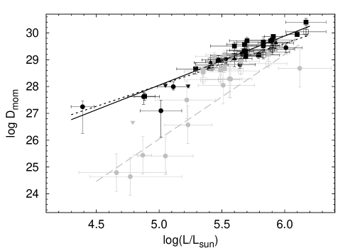
Figure 1: Modified wind-momentum – luminosity distribution of Galactic stars. Different luminosity classes are shown using circles, triangles and squares for, respectively, V, III-II and I class objects. Upper limits are shown as inverted triangles. Black/grey symbols refer to fastwind/cmfgen analyses. Clumping corrected $D_{\rm mom}$ values, using a clumping correction of $-0.37$ dex for objects with a H$\alpha$ emission line profile, are shown with open symbols. Left: stars analysed by Mokiem et al. (2005) using an automated fitting method. The solid line corresponds to the empirical wind-momentum luminosity relation (WLR) for rates not corrected for clumping. A dotted line is the WLR for clumping corrected values. Right: total Galactic sample. Black solid and dotted lines, respectively, correspond to WLRs fitted to the complete sample using uncorrected and clumping corrected rates. The grey dashed line is the WLR obtained from fitting only the dwarfs analysed by Martins et al. (2005), adopting their rates for $f=1$ (grey circles). Upper limits were not considered in determining any of the best fits.

For the Galaxy we consider a sample based on the analyses performed by Repolust et al. (2004), Mokiem et al. (2005), Martins et al. (2005) and Crowther et al. (2006). Note that the second study includes a reanalysis of the Cyg OB2 stars analysed by Herrero et al. (2002), and HD 15629 and $\zeta$ Oph studied by Repolust et al. The relevant atmospheric parameters adopting non-clumped mass-loss rates are listed in Tab. 4. Two entries are given for HD 15629 and HD 93250, as they were analysed separately using fastwind and cmfgen. In the following determination of the Galactic WLR, we adopt the results of the fastwind studies for reasons of consistency, but note that the differences of both analyses are not signficant.

In Fig. 1 the distribution of the Galactic stars in the modified wind-momentum vs. luminosity diagram is presented, where black/grey symbols refer to fastwind/cmfgen analyses. Different luminosity classes are distinguished using circles, triangles and squares for, respectively, class V, III-II and I objects. The open symbols show $D_{\rm mom}$ values resulting from scaling the $\dot{M}$ by a factor of 0.44, corresponding to $-$0.37 in $\log\mbox{$D_{\rm mom}$}$, for supergiants exhibiting H$\alpha$ emission line profiles. A reduction of this amount was proposed by Repolust et al. (2004) to correct for the fact that these stars have a systematically higher wind momentum compared to O dwarfs and theoretical predictions (see also Puls et al., 2003; Markova et al., 2004). The physical interpretation for this systematic offset proposed by these authors is connected to wind clumping. Because H$\alpha$ is a recombination line, its strength scales with the (wind)density $\rho$ squared. In a uniformly clumped wind, the emission will increase by a factor $f=<\rho^{2}>/<\rho>^{2}$, where $f$ is referred to as the clumping factor. As the H$\alpha$ line-forming region of stars with H$\alpha$ in emission is more extended compared to stars in which the profile is seen in absorption, these more extended regions must be more clumped than the innermost wind regions of those stars with absorption type profiles. In this interpretation, therefore, the observed offset suggests a (spatial) gradient in the clumping factor or a difference in the clumping properties of thin and thick winds. The (differential) clumping factor that corresponds to the applied scaling is $f=1/0.44^{2}\simeq 5$. We will return to the issue of clumping in Sect. 8.2.

The left-hand side of Fig. 1 compares the stars that have been analysed by Mokiem et al. (2005) in a homogeneous way by using an automated fitting method. We have constructed a WLR by fitting a power law, while accounting for both the symmetric errors in $L_{\star}$ and the asymmetric errors in $D_{\rm mom}$, to the observed distribution. This empirical WLR is shown as a solid and dotted black line for uncorrected and clumping corrected wind momenta, respectively. The clumping corrected relation is found to be flatter because the clumping corrections only affected the two brightest objects. In Sect. 7 we will compare the empirical and theoretical WLRs in the observed $L_{\star}$ range.

On the right-hand side of Fig. 1 the observed $D_{\rm mom}$ distribution for the complete Galactic sample is shown. The empirical WLRs determined for this sample are again shown as a black solid and dotted line for the uncorrected and clumping-corrected rates. As can be seen in Tab. 3 the fit coefficients for both relations are in very good agreement with those derived from the homogeneously analysed sample.

The Galactic sample comprises results from both cmfgen and fastwind studies. We note that fastwind is so far limited to studies of the visual spectral region – therefore H$\alpha$ is the most important $\dot{M}$ diagnostics – while cmfgen (also) uses the ultraviolet regime. In the latter approach the UV lines are given more weight in the mass-loss determination. In the case of weak winds ($\lesssim 10^{-7}M_{\odot}{\rm yr}^{-1}$) the $\dot{M}$ determinations rely almost exclusively on fits to C iv $\lambda\lambda 1548,1551$ (Martins et al., 2005).

Figure 1 shows good agreement between cmfgen and fastwind studies for relatively high luminosities ($\log L_{\star}/L_{\odot}\gtrsim 5.5$), consequently high wind densities. For lower luminosities, the UV analyses of the dwarf sample studied by Martins et al. (2005) show a systematic discrepancy with the average relations. This is emphasised by the grey dashed line, which shows the average relation for these objects. The fit coefficients of this latter relation are also listed in Tab. 3 and clearly signal a discrepency between UV based mass-loss determinations and theoretical expectations. This is referred to as the “weak wind problem” (see e.g. Bouret et al., 2003). We will discuss this further in Sect. 8.1.

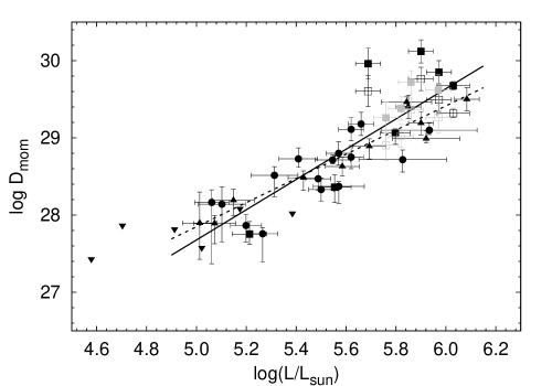
Figure 2: Modified wind momentum – luminosity distribution for LMC stars. Symbols have the same meaning as in Fig. 1. Left: stars analysed by Mokiem et al. (2007) using an automated fitting method. Dotted and dashed lines are empirical WLRs fitted to uncorrected and clumping corrected $D_{\rm mom}$ values, respectively. Right: total LMC sample. Fitted empirical WLRs are shown as a solid and dashed line for uncorrected and clumping corrected wind momentum rates. The fit coefficients for the different WLR relations are given in Tab. 3. Upper limits were not considered in determining any of the best fits.

6.2 LMC

The studies from which we have drawn the LMC sample are those of Crowther et al. (2002), Massey et al. (2004, 2005), Evans et al. (2004a) and Mokiem et al. (2007). In Tab. 5 the relevant atmospheric parameters are listed. Note that some of the objects in this table have been analysed in more than one study. In those cases we adopted the results from studies using the automated fitting procedure developed by Mokiem et al. (2005). If these were not available we preferred results from studies that used both the optical and UV spectral range over results that consider only the optical regime. For a number of stars analysed by Mokiem et al. (2007), no UV measurement of the wind velocity was available. Consequently, these authors estimated $v_{\infty}$ by scaling the escape velocity at the stellar surface ($v_{\rm esc}$) with a constant factor of 2.6 (cf. Lamers et al., 1995). To account for the metallicity dependence and to facilitate a comparison with theoretical predictions, we accordingly rescaled this $v_{\infty}$ using Eq. 3 with $Z=0.5\,Z_{\odot}$ and $n=0.13$ (cf. Leitherer et al., 1992). In Tab. 5 the rescaled values are given between brackets. As $v_{\infty}$ also influences the density in the line forming region of wind sensitive lines (because of the requirement of mass continuity), also a rescaling of $\dot{M}$ was required. For this we used the wind-strength parameter

$$Q=\frac{\dot{M}}{R^{3/2}_{\star}v_{\infty}}\leavevmode\nobreak\ .$$ (5)

that conserves the H$\alpha$ equivalent width (Schmutz et al. 1989, see also Puls et al. 1996 and de Koter et al. 1997). The combined effect of these re-scalings is a reduction of the modified-wind momentum by 0.08 dex.

The distribution of the modified-wind momenta as a function of stellar luminosity for the LMC stars is shown in Fig. 2 using the same symbols as in Fig. 1. On the left-hand side of the figure we (again) only consider objects that have been analysed by Mokiem et al. (2007) using an automated fitting method. The solid and dotted lines give the mean relations for uncorrected and clumping corrected rates. The correction applied was the same as for the Galactic stars. We note however that the metallicity dependence of this correction is as yet unknown.

For the total sample, shown on the right-hand side of the Fig. 2, the scatter is slightly larger. In particular the bright supergiants Sk $-67$ 22 at $\log L_{\star}/L_{\odot}\approx 5.7$ seems to stand out. Probably its discrepant position can be explained by the fact that Massey et al. (2005) could only determine a lower limit for its effective temperature, hence it could be intrinsically brighter. Despite the increased scatter, the obtained WLRs are in good agreement with the relations determined from the homogeneously analysed sample. This can be seen from the fit coefficients given in Tab. 3. For a confrontation of the empirical behaviour of the WLR with predictions, we refer the reader to Sect. 7.

6.3 SMC

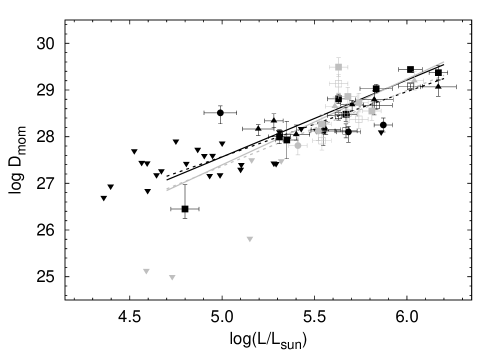
Figure 3: Modified wind momentum – luminosity distribution for SMC stars. The symbols have the same meaning as in Fig. 1. To construct the uncorrected and clumping corrected empirical WLR (solid and dashed line) the dwarf NGC346 033 at $\log L_{\star}/L_{\odot}\approx 5.0$ was not taken into account as the scaling of the escape velocity resulted in an anomalously high wind velocity. In Tab. 3 the fit coefficients for the individual relations are listed. Left: stars analysed by Mokiem et al. (2006) an automated fitting method. Right: total SMC sample. It turns out that the WLR is strongly influenced by the objects with $\log L_{\star}/L_{\odot}<5.3$. This is shown by the grey lines, which correspond to the empirical WLRs calculated ignoring these objects. For establishing the empirical $\dot{M}(Z)$ as well as for the comparison with theory we will use the latter set of WLRs. Upper limits were not considered in determining any of the best fits.

In Tab. 6 atmospheric parameters are given for the SMC sample that was compiled from the studies of Hillier et al. (2003), Bouret et al. (2003), Trundle et al. (2004), Massey et al. (2004), Evans et al. (2004a), Trundle & Lennon (2005), Massey et al. (2005) and Mokiem et al. (2006). For objects that were fitted in multiple studies we adopted results of one of these investigations following the same rules as applied to the LMC stars. Wind velocities given between brackets correspond to values that were calculated from the escape velocity at the stellar surface. These velocities and the associated mass-loss rates were scaled in a similar manner as was done for the LMC. Adopting $Z=0.2\,Z_{\odot}$, the $D_{\rm mom}$ values were scaled down by 0.18 dex.

Figure 3 shows the distribution of the SMC stars in the $D_{\rm mom}$ vs. $L_{\star}$ diagram. The symbols used are the same as in Fig. 1. On the left-hand side of the figure only the objects that have been analysed using an automated fitting method by Mokiem et al. (2006) are shown. For $\log L_{\star}/L_{\odot}\lesssim 5.3$ the majority of the mass-loss determinations are upper limits. The empirical WLRs are shown using a solid and dotted line for uncorrected and clumping corrected wind momenta. Note the position of the dwarf NGC346-033 at $\log L_{\star}/L_{\odot}\approx 5.0$. We did not include this object in the fits, as its high wind momentum is the result of an anomalously high wind velocity resulting from the scaling with $v_{\rm esc}$ (also see Mokiem et al., 2006).

The right-hand side of Fig. 3 shows the wind momentum distribution for the total SMC sample. For this large sample the low luminosity part of the diagram still remains scarcely populated. Also note the upper limits determined using cmfgen for $\log L_{\star}/L_{\odot}<5.2$. This could point to a steeper WLR relation for UV based mass-loss estimates compared to those obtained from H$\alpha$, as was found for the galactic case. However, this is not a firm statement as by far the bulk of the SMC targets in this luminosity range only show upper limits.

The empirical WLRs for the total sample are shown on the right-hand side Fig. 3 as a black solid line for uncorrected wind momenta and as a dotted line for clumping corrected values. We find that these relations are strongly influenced by the objects with $\log L_{\star}/L_{\odot}<5.3$. This is shown by the grey solid and dashed lines, which correspond to the respective WLRs calculated ignoring these objects. As the low luminosity part of the SMC diagram is rather uncertain, we opted to use this latter set of relations. Note that this choice will not influence our determination of the metallicity dependence of $\dot{M}$, as this will be based on the stars brighter than $L_{\star}$/$L_{\odot}$= 5.3. In this range, the fit uncertainties are small (see Sect. 7).

7 Mass loss versus metallicity

Now that we have established the empirical modified-wind momentum luminosity relation for the three galaxies, we can determine the $\dot{M}(Z)$ relation. Before doing so, we first inter compare the results for these three environments, and confront them with predictions.

7.1 Global comparison

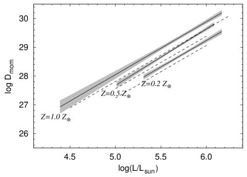
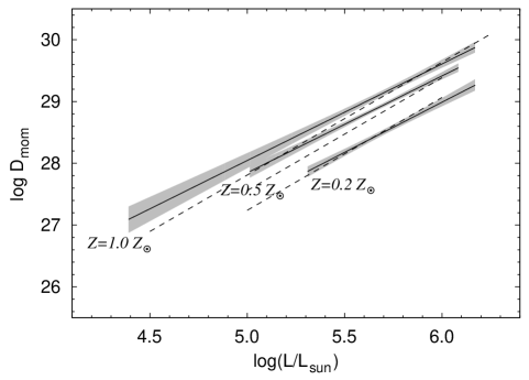
Figure 4: Comparison of the observed wind momentum – luminosity relations (solid lines) with the predicted relations of Vink et al. (2000, 2001) (dotted lines). Top, middle and bottom lines of each line style, respectively, correspond to Galactic, LMC and SMC observed and predicted WLRs. Left and Right plots show, respectively, empirical WLRs including uncorrected and clumping corrected wind momentum rates. See Sect. 6.1 for the applied clumping correction. One sigma confidence intervals for the empirical relations are shown as grey areas.

In Fig. 4 the empirical modified-wind momentum relations determined for the total observed samples (solid lines) are shown alongside the predicted relations of Vink et al. (2000, 2001) (dotted lines). The top, middle and bottom lines of each line style, respectively, correspond to the Galactic, LMC and SMC observed and predicted relations. To facilitate a meaningful comparison one sigma confidence intervals for the observed WLRs are shown as grey areas. First focusing on the left-hand side, showing the relations without a clumping correction, we see that the empirical relations are clearly separated from each other beyond the fitting uncertainties. We interpret this as quantitative evidence for a successive decrease of the mass-loss rates of massive stars in the Galactic, LMC, and SMC environment.

For the entire investigated luminosity range, the relative separations of the empirical WLRs agree well with the separations predicted by Vink et al. (2001), although the empirical WLRs do show a systematic offset compared to the theoretical results. Focusing for a moment on the relative separations only: measured at $\log L_{\star}/L_{\odot}=5.75$, which coincides with the region where the fit uncertainties are the smallest, the offsets between the empirical and theoretical relations relative to the Galaxy are: $0.28$ and $0.25$ for the LMC, and $0.62$ and $0.57$ for the SMC.

The systematic offset between observations and theory is of the order of 0.2 dex. This suggests that if wind clumping does affect the determination of empirical mass-loss rates, but would only have a marginal effect on mass-loss predictions, the empirical mass-loss rates would be overestimated by at most a factor of $\sim$ two.

Indeed, when turning to the clumping corrected empirical relations, the relative offset almost disappears. This is shown on the right-hand side of Fig. 4, where we show the wind momentum relations obtained from the total observed samples accounting for this correction. Note that, strictly speaking, this agreement pertains only to stars not showing H$\alpha$ in emission, as the clumping corrections is designed such as to scale the ones that do show H$\alpha$ emission to those that do not (see Sect. 6.1). The slopes of the empirical relations, however, are slightly flatter, as the clumping correction preferentially affects the high-luminosity objects.

7.2 The empirical $\dot{M}(Z)$ relation

To calculate the mass loss metallicity dependence we use the relative separation between the empirical modified-wind momentum relations at $\log L_{\star}/L_{\odot}=5.75$, for which the fit uncertainty in all three relations is at its minimum. Note that the differential slopes also allow for a luminosity dependent $Z$-dependence, however, based on the uncertainties we doubt whether this would be meaningful. Moreover, for the SMC it was shown that this slope is very sensitive to the rather uncertain low luminosity domain. In Tab. 3 the power law indices for the observed $\dot{M}(Z)$ dependence for the LMC and SMC relative to the Galaxy are listed. These were calculated using Eq. 4 assuming $n=0.13$. The indices determined from the homogeneously analysed sample are in good agreement with those determined for the total sample. For the LMC relatively larger differences are found compared to the SMC, which is a result of the smaller metallicity difference of this system relative to our galaxy. This also explains the larger error bars.

To determine the global metallicity dependence, we made a linear fit regarding the logarithm of the differential (i.e. with respect to the Galaxy) modified wind momentum and the log of the differential metallicity. Assuming smooth winds, we find:

$$\dot{M}\propto Z^{0.83\pm 0.16}\leavevmode\nobreak\ .$$ (6)

We emphasize that the error bar in $m$ is a fitting error of the mass-loss rate and the metallicity only. Several uncertainties add to the quoted error. These include i) those related to the adopted luminosity at which we gauge the relation; ii) errors related to the neglect of the correlation between luminosity and modified wind momentum (Markova et al., 2004, see); iii) errors related to uncertainties in the $v_{\infty}$($\dot{M}$) dependence, i.e. in the adopted value $n=0.13$, and iv) those related to possible systematic uncertainties in the metallicities of the Magellanic Clouds. The motivation for gauging at $\log L_{\star}/L_{\odot}=5.75$ is given above. Least squares fit analysis including the correlation between $L$ and $D$ yield similar results for the stars analysed using the automated fitting method, though for the total sample the Galactic $\log D(\log L)$ relation is found to be somewhat steeper. Deviations in the Galactic slope are to be expected (Markova et al., 2004). However, at $\log L_{\star}/L_{\odot}=5.75$ the wind momenta are not found to be very different and result in uncertainties $\Delta m\lesssim 0.10$ dex. Uncertainties in the velocity vs. metallicity dependence are not very well known, however, they are likely to be small as well. By far the largest source of error in $m$ is that due to uncertainties in the metallicities of the Magellanic Clouds, notably that of the SMC. To illustrate this, if the SMC metal content is not $\Delta[Z/{\rm H}]\sim-0.7\pm 0.1$ but rather $-0.5\pm 0.1$, the empirical value of $m$ will increase to $1.13\pm 0.25$.

Keeping this in mind, the derived exponent $m$ of the empirical mass-loss luminosity relation as given in Eq. 6 appears to be consistent with the predicted value of $m_{\rm pred}=0.69\pm 0.10$ (Vink et al., 2001) and $m_{\rm pred}=0.67$ from the alternative investigation by Krtička (2006).

If we apply the earlier-mentioned clumping correction scaling of $-$0.37 dex in $\log\mbox{$D_{\rm mom}$}$ for stars showing H$\alpha$ emission, the metallicity dependence is found to be:

$$\dot{M}\propto Z^{0.72\pm 0.15}\leavevmode\nobreak\ .$$ (7)

This result too is consistent with both theoretical predictions quoted above.

Three remarks need to be made. First, we can only state that this $\dot{M}(Z)$ relation holds for stars more luminous than $\sim$$10^{5.2}$ $L_{\odot}$. The reasons are the lack of firm $\dot{M}$ determinations for stars less luminous than this number and the inconsistency between the H$\alpha$ and UV wind lines mass-loss diagnostics (see below). Note in particular that the slope of the WLR might depend on the wind-density and/or metallicity itself (as it is predicted from a close inspection of the line-strength distribution functions, cf. Puls et al. 2000), though not to such an extent as indicated by the weak wind problem (cf. Fig. 1). In so far, it is possible that the metallicity dependence for low-luminosity objects deviates from our previous results.

Second, the absolute agreement in wind momentum only holds if the winds of the O dwarfs are not significantly clumped. If they are, the predictions (which do not yet account for clumping) may overestimate the mass-loss rate and therefore $D_{\rm mom}$. Third, if O dwarf winds are clumped, but the clumping does not depend on metal content or mass-loss (i.e. $f\neq f(Z,\dot{M}(Z))$) then the derived $m$ will not be affected, and, therefore, the agreement in the observed and predicted mass loss – metallicity scaling will remain preserved. To rephrase this last point: irrespective of what the actual $\dot{M}$ values are, if clumping were independent of metallicity and wind density, the derived power-law index is anticipated to be correct – even if the winds are significantly clumped.

Interestingly, these analyses suggest that the systematic errors in the slope of the mass-loss-metallicity relation, $m$, as introduced by potential wind clumping may be less relevant than remaining uncertainties in the metallicity determinations of the Magellanic Clouds.

8 Discussion

8.1 The weak wind problem

As mentioned before, for the majority of stars at lower luminosities the ultraviolet resonance lines based mass-loss rates disagree strongly with theoretical predictions. Still, there are few (though different) Galactic objects at similar, low luminosity which display a “normal” H$\alpha$ mass-loss rate, which might point either to different physics or questions the validity of at least one of the applied diagnostical tools.

Going from high to low luminosity, figures 1 and 3 show that this discrepancy appears at $L_{\star}\approx 10^{5.25}\,L_{\odot}$. The dwarf star sample recently analysed by Martins et al. (2005) using cmfgen suggests progressively weaker winds than are predicted by current theory. At $L\sim 10^{4.75}L_{\odot}$ this discrepancy has reached a factor 100. Note that given the still limited number of stars investigated at relatively low luminosity alternative descriptions (compared to a steeper slope) of the WLR might also be appropriate. For instance, the WLR may retain the same slope but jump to a two order of magnitudes lower value of $D_{\rm mom}$ at $L\lesssim 10^{5.25}\,L_{\odot}$ compared to the predictions. In the SMC, the discrepancy could be even worse, as UV analyses only yield upper limits. Note that also the H$\alpha$ analyses of SMC objects at $L\lesssim 10^{5.25}\,L_{\odot}$ yield almost exclusively results as upper limits. So, in principle, these need not be contradictory to the UV based $\dot{M}$.

What could be the reason for this “weak wind problem”? There are three directions in which one might look for causes: first, errors in the H$\alpha$ and/or UV analysis; second, missing physics or invalid assumptions in the wind predictions, or, third, the nature of the stars showing the weak wind problem is different from that of normal OB stars (that do appear to follow theory). Here, we focus on the first possibility. For more thorough discussions on this topic we refer to Martins et al. (2004, 2005) and de Koter (2006).

Two important advantages of the H$\alpha$ method are that the ionisation and abundance of hydrogen are well known. One cannot make this statement with similar confidence for the elements responsible for the UV resonance lines. For the weak wind stars, the prime $\dot{M}$ diagnostic – C iv as mentioned – is only a trace ion, i.e. it does not represent the dominant ionisation stage. This makes it is susceptible to X-ray emission, thought to originate from shocks that may develop in the wind outflow. Martins et al. (2005) present test calculations estimating that X-rays may decrease the C iv ionisation by an order of magnitude, requiring an increase of the mass loss by the same amount to preserve the line fit. With typical uncertainties in the carbon abundance of a factor of two, this shows that the UV method is much more prone to errors than the H$\alpha$ method. This does not imply that H$\alpha$ does not suffer from uncertainties. Besides the ambiguity in $\dot{M}$ introduced by the unknown velocity law in weaker winds which has been discussed already, continuum rectification issues and potential nebular emission limit the applicability of the H$\alpha$ diagnostic to stars with $\dot{M}\gtrsim 10^{-7}M_{\odot}{\rm yr}^{-1}$. To reach this limit requires high signal-to-noise data of stars with no appreciable nebular emission, such as is the case for three of the five Galactic stars at $L\lesssim 10^{5.15}\,L_{\odot}$ – i.e. in the (UV identified) weak wind regime. These galactic stars are $\zeta$ Oph, Cyg OB2 #2, and HD 217086. For two other stars at these low luminosities, $\tau$ Sco and 10 Lac, we also established the mass-loss rate, however, the error bars on these determinations are large. For the three stars mentioned, the H$\alpha$ derived rates do appear to be more or less consistent with predictions. Note that some of the C iv analyses account for (canonical) X-ray emission suggesting that the problem may not be fully explicable by uncertainties in the UV method.

So far the origin of the weak wind problem has not yet been identified. We stress that because of the poor overlap between the H$\alpha$ and UV diagnostics, it is at present difficult to exclude the possibility that the (major) cause is simply connected with uncertainties in the wind structure predicted by the model atmospheres that are needed to derive the empirical $\dot{M}$– notably the ionisation of species responsible for the UV resonance lines. Further spectroscopy in the IR, particularly using Br$\alpha$ as an ideal mass-loss indicator also for weak winds, might unravel at least part of the problem.

8.2 Small-scale clumping

So far, we have not discussed the physical reality of the “clumping” correction applied in Sect. 6 to bring the WLR relation of the supergiants with H$\alpha$ emission line profiles in accord with those of dwarfs. Is wind clumping observed in O stars? And, is clumping more important in the winds of supergiants? Clumping was studied in detail by Hillier (1991) to explain the scattering wings of He ii lines of Wolf-Rayet stars. Although these stars are known to have very dense winds, their He ii scattering wings are weak features. Consequently, for the weaker O star winds these diagnostics cannot be applied. Nonetheless, direct observational evidence that the winds of O stars are also clumped was provided by Eversberg et al. (1998) from time series spectroscopy of He ii $\lambda 4686$ in $\zeta$ Pup, and by Crowther et al. (2002); Hillier et al. (2003); Bouret et al. (2003); Massa et al. (2003); Martins et al. (2004, 2005); Bouret et al. (2005), and Fullerton et al. (2006) from analysis of UV (resonance) lines, partly in combination with optical lines.

The fitting of the ultraviolet lines, notably P v $\lambda\lambda 1118,1128$, O v $\lambda 1371$, and N iv $\lambda 1718$, is found to be improved if a distance dependent clumping is introduced – with clumps starting to form above the sonic point and reaching maximum clumping in the outer wind – and a void interclump medium is assumed. In the above listed studies a total of 25 stars have been analysed using the cmfgen code. Clumping corrections are applied in roughly half the sample, including both dwarfs and supergiants – for objects brighter than $10^{5.15}L_{\odot}$. The maximum clumping factors that are derived from these studies are in the range 10 – 100. Though clumping corrections have turned out to be necessary for some stars but not for others, this does not exclude the possibility that all stars are clumped to a certain degree: Due to the fact that only few lines react differentially on clumping and thus allow for distinct statements, it is rather difficult to exclude the presence of clumping in a certain object at the present state of knowledge unless the wavelength coverage is fairly complete (extending from the UV to the IR), and unless a large number of systematic investigations have been performed.

In addition to these purely spectroscopic investigations, Puls et al. (2006) analyzed a sample of Galactic O-type (super)giants more recently, combining H$\alpha$, infrared, mm and radio fluxes to derive constraints on the radial stratification of the clumping factor. Since all diagnostics employed have a $\rho^{2}$ dependence, only relative clumping factors could be derived, normalized to the values in the outermost, radio-emitting region, whereas absolute values for the clumping factors and thus the actual mass-loss rates remained unconstrained.

In contrast to present hydrodynamical simulations of the line-driving instability but in (partial) agreement with previous studies it was found that for denser winds clumping starts fairly close to the sonic point, reaches a certain maximum (mostly within $r<2\mbox{$R_{\star}$}$) and decreases outwards, where the maximum, normalized clumping factors are of the order of 3 to 6. For weaker winds, on the other hand, the clumping factors in the inner and outermost regions turned out to be similar.

This appears to be consistent with findings from the linear polarimetry of Luminous Blue Variables (Davies et al., 2005), where it was found that (i) clumping must start close to the photosphere to reproduce the observed levels of polarimetry, and (ii) denser winds yield a larger amount of linear polarisation (see also Robert et al., 1989, for WR stars).

The results by Puls et al. (2006) could mean one of two things: either the outer wind is significantly clumped whilst the inner wind is even more strongly clumped (which would imply that the UV results calling for large clumping factors are correct), or the outer wind is not significantly clumped and the current mass-loss predictions are approximately correct. The latter possibility, of course, would require an explanation of the different UV results.

8.3 Concluding remarks

The first result we mention is that the empirical $\dot{M}(Z)$ relation appears to be in agreement with theoretical predictions for luminosities larger than $\sim$$10^{5.2}$ $L_{\odot}$. Second, for lower luminosities, UV based $\dot{M}$ determinations for dwarfs seem to indicate a breakdown of the theory, leading to discrepancies of up to a factor $10^{2}$ for the lowest luminosity stars with a measurable mass loss. We found that for the H$\alpha$ based mass-loss rates of three galactic stars, $\zeta$ Oph, Cyg OB2 #2, and HD 217086, do follow the predictions down to $\log L_{\star}/L_{\odot}\approx 4.9$. Their $\dot{M}$ values are $\sim 2\times 10^{-7}\leavevmode\nobreak\ M_{\odot}{\rm yr}^{-1}$ or less, which is so low that they may suffer from uncertainties that are not reflected in the derived error bars, for instance those associated with the uncertain velocity law in low density winds and/or the unnoticed presence of minor amounts of nebular emission. Still, given these findings, it appears premature to exclude the possibility that the (major) cause of the breakdown between empirical and predicted mass loss at low luminosity is connected to modeling uncertainties associated with the empirical $\dot{M}$ values.

To further probe the cause of the possible theoretical breakdown at low luminosity, it is therefore necessary to study those stars for which both the H$\alpha$ and UV line indicators of mass loss can be applied – although unfortunately there is only a very limited mass-loss regime for which this is possible. To this end, the use of Br$\alpha$ as a mass-loss diagnostic (Lenorzer et al., 2004; Repolust et al., 2005) will prove to be fruitful as it will widen the overlap between hydrogen and UV line analyses. Regarding clumping, the P v resonance line seems a powerful diagnostic (Massa et al., 2003; Fullerton et al., 2006). Also, it may be fruitful to focus on the question whether all O-type stars suffer from clumping. Concerning the effect of clumping on the mass loss vs. metallicity relation, the following important remark can be made: regardless what the actual $\dot{M}$ values are, if clumping is universal in O-type stars, and if it does not depend on wind properties such as density or metallicity, then the derived scaling (i.e. the power law index $m$) remains correct.

Finally, let us briefly contemplate some implications of O-type star mass-loss rates that are lower by factors of 3 to 100 than so far assumed. These implications branch out into at least two directions: wind hydrodynamics and stellar evolution. For our understanding of the intrinsic instabilities associated with the wind driving mechanism (Owocki, 1994) the requirement of clumping factors $f\sim 10-100$ in the H$\alpha$ line forming regions of dwarf O-type stars, which do not extend far beyond the sonic point, seems to imply that these density inhomogeneities have developed already in the sub-sonic part of the flow. As an example, the O5 V star N11-051 in the LMC has an H$\alpha$ line forming region that extends from the photosphere to a velocity of 13 km s^-1, which is about 0.6 times the sonic velocity. For other O-type dwarfs, similar results are found. This is not anticipated by theory, which predicts that the onset of line-driven instabilities is only at about the sonic velocity (where, admittedly, the growth rate of the instability is large). Implications for the wind driving mechanism may also be severe, although it should be noted that clumping has not yet been incorporated in mass-loss predictions.

Clumping may also impact on our understanding of massive star evolution. Weaker stellar winds will cause less loss of angular momentum. Consequently the stars will not spin down as rapidly as currently thought. It may even be expected that most Galactic massive stars retain their initial rotational velocity properties during the entire main sequence (Meynet & Maeder, 2000; Maeder & Meynet, 2001). For the brightest stars – corresponding to initial masses of 60 $M_{\odot}$ or more – the integrated main-sequence mass loss could drop dramatically. With the current rates they are expected to lose 20 to 40 percent of their mass in the H-burning phase. This could drop by a factor of three, requiring the objects to lose ten to tens of solar masses by other means in order to evolve towards the hot Wolf-Rayet phase Smith & Owocki (2006). This could either imply an increase of the duration of the LBV phase by a factor of two, assuming that the (unknown) mechanism thought to be responsible for the eruptive mass loss in this phase is unaffected by clumping issues (see e.g. Humphreys & Davidson, 1994), or alternatively that some LBVs explode before reaching the Wolf-Rayet phase (Kotak & Vink, 2006; Gal-Yam et al., 2007; Smith, 2007).

Appendix A Parameters analysed samples

Table 4: Wind parameters of Galactic O- and early B-type stars.

Star	ST	$T_{\rm eff}$	$R_{\star}$	$\log L_{\star}$	$\dot{M}$	$v_{\infty}$	$\log\mbox{$D_{\rm mom}$}$	Ref.
		[kK]	[$R_{\odot}$]	[$L_{\odot}$]	[$M_{\odot}{\rm yr}^{-1}$]	[km s-1]	[${\rm g\,cm\,s^{-2}}\,R_{\odot}$]
Cyg OB2 #7	O3 If∗	45.8	14.2	5.91	$9.98\cdot 10^{-6}$	3080	29.867	2
Cyg OB2 #11	O5 If+	36.5	21.9	5.89	$7.36\cdot 10^{-6}$	2300	29.700	2
Cyg OB2 #8C	O5 If	41.8	13.1	5.69	$3.37\cdot 10^{-6}$	2650	29.313	2
Cyg OB2 #8A	O5.5 I(f)	38.2	25.5	6.10	$1.04\cdot 10^{-5}$	2650	29.943	2
Cyg OB2 #4	O7 III((f))	34.9	13.8	5.40	$8.39\cdot 10^{-7}$	2550	28.698	2
Cyg OB2 #10	O9.5 I	29.7	30.1	5.79	$2.63\cdot 10^{-6}$	1650	29.175	2
Cyg OB2 #2	B1 I	28.7	11.1	4.88	$1.63\cdot 10^{-7}$	1250	27.635	2
10 Lac	O9 V	36.0	8.4	5.01	$6.06\cdot 10^{-8}$	1140	27.098	2
$\zeta$ Oph	O9 V	32.1	8.9	4.88	$1.43\cdot 10^{-7}$	1550	27.621	2
$\tau$ Sco	B0.2 V	31.9	5.0	4.39	$6.14\cdot 10^{-8}$	2000	27.245	2
HD 115842	B0.5Ia	25.5	34.2	5.65	$2.00\cdot 10^{-6}$	1180	28.940	4
HD 122879	B0Ia	28.0	24.4	5.52	$3.00\cdot 10^{-6}$	1620	29.180	4
HD 14947	O5 If+	37.5	16.8	5.70	$8.52\cdot 10^{-6}$	2350	29.710	1
HD 152234	B0.5Ia(Nwk)	26.0	42.4	5.87	$2.70\cdot 10^{-6}$	1450	29.210	4
HD 15558	O5 III(f)	41.0	18.2	5.93	$5.58\cdot 10^{-6}$	2800	29.620	1
HD 15629	O5 V((f))	42.0	12.4	5.64	$9.28\cdot 10^{-7}$	3200	28.822	2
HD 15629	O5 V((f))	41.0	12.0	5.56	$3.16\cdot 10^{-7}$	2800	28.290	3
HD 18409	O9.7 Ib	30.0	16.3	5.29	$1.02\cdot 10^{-6}$	1750	28.660	1
HD 190864	O6.5 III(f)	37.0	12.3	5.41	$1.39\cdot 10^{-6}$	2500	28.890	1
HD 192639	O7 Ib(f)	35.0	18.7	5.68	$6.32\cdot 10^{-6}$	2150	29.570	1
HD 193514	O7 Ib(f)	34.5	19.3	5.68	$3.48\cdot 10^{-6}$	2200	29.330	1
HD 193682	O5 III(f)	40.0	13.1	5.60	$1.73\cdot 10^{-6}$	2800	29.040	1
HD 203064	O7.5 III:n((f))	34.5	15.7	5.50	$1.41\cdot 10^{-6}$	2550	28.950	1
HD 207198	O9 Ib	33.0	16.6	5.47	$1.79\cdot 10^{-6}$	2150	28.990	1
HD 209975	O9.5 Ib	32.0	22.9	5.69	$2.15\cdot 10^{-6}$	2050	29.120	1
HD 210809	O9 Iab	31.5	21.2	5.60	$5.30\cdot 10^{-6}$	2100	29.510	1
HD 210839	O6 I(n)fp	36.0	21.1	5.83	$6.85\cdot 10^{-6}$	2250	29.650	1
HD 217086	O7 Vn	38.1	8.4	5.11	$2.13\cdot 10^{-7}$	2550	27.995	2
HD 24912	O7.5 III(n)((f))	35.0	14.0	5.42	$1.08\cdot 10^{-6}$	2450	28.800	1
HD 303308	O4 V((f+))	41.0	11.5	5.53	$1.63\cdot 10^{-6}$	3100	29.030	1
HD 30614	O9.5 Ia	29.0	32.5	5.83	$6.04\cdot 10^{-6}$	1550	29.530	1
HD 34078	O9.5 V	33.0	7.5	4.77	$3.00\cdot 10^{-10}$	800	24.640	3
HD 37128	B0Ia	27.0	24.0	5.44	$2.25\cdot 10^{-6}$	1910	29.120	4
HD 38666	O9.5 V	33.0	6.6	4.66	$3.00\cdot 10^{-10}$	1200	24.790	3
HD 38771	B0.5Ia	26.5	22.2	5.35	$9.00\cdot 10^{-7}$	1525	28.610	4
HD 42088	O6.5 Vz	38.0	9.6	5.23	$1.00\cdot 10^{-8}$	1900	26.570	3
HD 46202	O9 V	33.0	8.4	4.87	$1.30\cdot 10^{-9}$	1200	25.440	3
HD 46223	O4 V((f+))	41.5	11.9	5.57	$3.16\cdot 10^{-7}$	2800	28.280	3
HD 66811	O4 I(f)	39.0	19.4	5.90	$8.80\cdot 10^{-6}$	2250	29.740	1
HD 91943	B0.7Ia	24.5	26.3	5.35	$7.50\cdot 10^{-7}$	1470	28.550	4
HD 91969	B0Ia	27.5	25.3	5.52	$1.00\cdot 10^{-6}$	1470	28.670	4
HD 93028	O9 V	34.0	9.7	5.05	$1.00\cdot 10^{-9}$	1300	25.410	3
HD 93128	O3 V((f))	46.5	10.4	5.66	$2.64\cdot 10^{-6}$	3100	29.220	1
HD 93129A	O2 If*	42.5	22.5	6.17	$2.63\cdot 10^{-5}$	3200	30.400	1
HD 93146	O6.5 V((f))	37.0	10.0	5.22	$5.62\cdot 10^{-8}$	2800	27.500	3
HD 93204	O5 V((f))	40.0	11.9	5.51	$1.78\cdot 10^{-7}$	2900	28.050	3
HD 93250	O3.5 V((f+))	46.0	15.9	6.01	$3.45\cdot 10^{-6}$	3250	29.450	1
HD 93250	O3.5 V((f+))	44.0	19.9	6.12	$5.62\cdot 10^{-7}$	3000	28.680	3
HD 94909	B0Ia	27.0	25.5	5.49	$2.00\cdot 10^{-6}$	1050	28.620	4

References: (1) Repolust et al. (2004); (2) Mokiem et al. (2005); (3) Martins et al. (2005); (4) Crowther et al. (2006)

Table 5: Wind parameters of O- and early B-type stars in the LMC. Wind velocities given between brackets are calculated from the escape velocity at the stellar surface. Identifications: “BI” from Brunet et al. (1975), “LH” from Lucke (1972), except LH 51-496, which is identified by Garmany et al. (1994), “N11” from Evans et al. (2006), “R136” from Hunter et al. (1997) and Massey & Hunter (1998) and “Sk” from Sanduleak (1970).

Star	ST	$T_{\rm eff}$	$R_{\star}$	$\log L_{\star}$	$\dot{M}$	$v_{\infty}$	$\log\mbox{$D_{\rm mom}$}$	Ref.
		[kK]	[$R_{\odot}$]	[$L_{\odot}$]	[$M_{\odot}{\rm yr}^{-1}$]	[km s-1]	[${\rm g\,cm\,s^{-2}}\,R_{\odot}$]
BI 237	O2 V((f*))	53.2	9.7	5.83	$7.81\cdot 10^{-7}$	3400	28.717	1
BI 253	O2 V((f*))	53.8	10.7	5.93	$1.92\cdot 10^{-6}$	3180	29.100	1
HD 2670952	O6 Iaf+	33.5	25.0	5.86	$1.10\cdot 10^{-5}$	1520	29.720	4
HD 269050	B0 Ia	24.5	42.2	5.76	$3.20\cdot 10^{-6}$	1400	29.260	5
HD 269896	ON9.7 Ia+	27.5	42.3	5.97	$7.50\cdot 10^{-6}$	1350	29.620	5
Lh101:W3-24	O3 V((f))	48.0	8.1	5.50	$5.00\cdot 10^{-7}$	2400	28.330	3
LH58-496	O5 V(f)	42.0	10.5	5.49	$6.00\cdot 10^{-7}$	2400	28.470	2
LH64-16	ON2 III(f*)	54.5	9.4	5.85	$4.00\cdot 10^{-6}$	3250	29.400	2
LH81:W28-23	O3.5 V((f+))	47.5	10.0	5.66	$2.50\cdot 10^{-6}$	3050	29.180	2
LH81:W28-5	O4 V((f+))	46.0	9.6	5.57	$1.20\cdot 10^{-6}$	2700	28.800	3
LH90:ST2-22	O3.5 III(f+)	44.0	18.9	6.08	$4.50\cdot 10^{-6}$	2560	29.500	2
N11-004	OC9.7 Ib	31.6	26.5	5.80	$1.62\cdot 10^{-6}$	[2182]	29.061	1
N11-008	B0.7 Ia	26.0	29.6	5.55	$4.53\cdot 10^{-7}$	[1480]	28.362	1
N11-026	O2 III(f*)	53.3	10.7	5.92	$1.66\cdot 10^{-6}$	[2848]	28.989	1
N11-029	O9.7 Ib	29.4	15.7	5.21	$1.58\cdot 10^{-7}$	[1440]	27.754	1
N11-031	ON2 III(f*)	45.0	13.7	5.84	$3.88\cdot 10^{-6}$	3200	29.462	1
N11-032	O7 II(f)	35.2	14.0	5.43	$7.37\cdot 10^{-7}$	[1752]	28.483	1
N11-033	B0 IIIn	27.2	15.6	5.07	$2.23\cdot 10^{-7}$	[1404]	27.891	1
N11-038	O5 II(f+)	41.0	14.0	5.69	$1.38\cdot 10^{-6}$	[2377]	28.890	1
N11-042	B0 III	30.2	11.8	5.01	$1.73\cdot 10^{-7}$	[2108]	27.896	1
N11-045	O9 III	32.3	12.0	5.15	$5.01\cdot 10^{-7}$	[1415]	28.191	1
N11-051	O5 Vn((f))	42.4	8.4	5.31	$9.27\cdot 10^{-7}$	[1927]	28.515	1
N11-058	O5.5 V((f))	41.3	8.4	5.27	$1.39\cdot 10^{-7}$	[2259]	27.758	1
N11-060	O3 V((f*))	45.7	9.7	5.57	$4.77\cdot 10^{-7}$	[2502]	28.371	1
N11-061	O9 V	33.6	11.7	5.20	$1.96\cdot 10^{-7}$	[1734]	27.865	1
N11-066	O7 V((f))	39.3	7.7	5.10	$3.73\cdot 10^{-7}$	[2116]	28.140	1
N11-068	O7 V((f))	39.9	7.1	5.06	$3.13\cdot 10^{-7}$	[2769]	28.164	1
R136-014	O3.5 If*	38.0	21.1	5.90	$2.30\cdot 10^{-5}$	2000	30.120	2
R136-018	O3 III	45.0	14.7	5.90	$2.00\cdot 10^{-6}$	3200	29.190	2
R136-033	O3 V	47.0	9.8	5.62	$2.00\cdot 10^{-6}$	3250	29.110	2
R136-055	O3 V	47.5	9.4	5.62	$9.00\cdot 10^{-7}$	3250	28.750	3
Sk $-65$ 47	O4 If	40.0	20.1	5.97	$1.20\cdot 10^{-5}$	2100	29.850	2
Sk $-66$ 169	O9.7 Ia+	26.0	40.0	5.82	$6.00\cdot 10^{-6}$	1000	29.380	4
Sk $-67$ 22	O2 If*	42.0	13.2	5.69	$1.50\cdot 10^{-5}$	2650	29.960	2
Sk $-66$ 100	O6 II(f)	39.0	13.6	5.58	$8.81\cdot 10^{-7}$	2075	28.629	1
Sk $-66$ 18	O6 V((f))	40.2	12.2	5.55	$1.07\cdot 10^{-6}$	2200	28.714	1
Sk $-67$ 166	O4 Iaf+	40.3	21.3	6.03	$9.28\cdot 10^{-6}$	1750	29.675	1
Sk $-70$ 69	O5 V	43.2	9.0	5.41	$1.03\cdot 10^{-6}$	2750	28.728	1

References: (1) Mokiem et al. (2007), (2) Massey et al. (2005), (3) Massey et al. (2004), (4) Crowther et al. (2002), (5) Evans et al. (2004a)

Table 6: Wind parameters of O- and early B-type stars in the SMC. Wind velocities given between brackets are calculated from the escape velocity at the stellar surface. Identifications: “AzV” from Azzopardi & Vigneau (1975, 1982), “MPG” from Massey et al. (1989) and “NGC330” and “NGC346” from Evans et al. (2006).

Star	ST	$T_{\rm eff}$	$R_{\star}$	$\log L_{\star}$	$\dot{M}$	$v_{\infty}$	$\log\mbox{$D_{\rm mom}$}$	Ref.
		[kK]	[$R_{\odot}$]	[$L_{\odot}$]	[$M_{\odot}{\rm yr}^{-1}$]	[km s-1]	[${\rm g\,cm\,s^{-2}}\,R_{\odot}$]
NGC346-001	O7 Iaf+	34.1	29.3	6.02	$6.04\cdot 10^{-6}$	1330	29.438	1
NGC346-007	O4 V((f))	41.5	11.1	5.52	$2.70\cdot 10^{-7}$	2300	28.120	3
NGC346-010	O7 IIIn((f))	35.9	10.2	5.20	$4.88\cdot 10^{-7}$	[1486]	28.166	1
NGC346-012	B1 Ib	26.3	12.1	4.80	$1.01\cdot 10^{-8}$	[1272]	26.450	1
NGC346-033	O8 V	39.9	6.6	4.99	$6.02\cdot 10^{-7}$	[3328]	28.510	1
NGC330-013	O8.5 III((f))	34.5	14.1	5.40	$2.96\cdot 10^{-7}$	1600	28.049	1
AzV 15	O7 II	39.4	18.3	5.82	$1.12\cdot 10^{-6}$	2125	28.791	1
AzV 26	O7 III	40.1	25.2	6.17	$1.71\cdot 10^{-6}$	2150	29.066	1
AzV 69	OC7.5 III((f))	33.9	18.6	5.61	$9.20\cdot 10^{-7}$	1800	28.650	5
AzV 70	O9.5 Ibw	28.5	28.4	5.68	$1.50\cdot 10^{-6}$	1450	28.860	2
AzV 75	O5.5 I(f)	40.0	25.4	6.17	$3.50\cdot 10^{-6}$	2100	29.370	4
AzV 83	O7 Iaf+	32.8	18.3	5.54	$2.00\cdot 10^{-6}$	940	28.270	5
AzV 95	O7 III	38.2	13.8	5.56	$3.56\cdot 10^{-7}$	1700	28.151	1
AzV 104	B0.5 Ia	27.5	20.0	5.31	$3.24\cdot 10^{-7}$	[1087]	27.998	6
AzV 215	BN0 Ia	27.0	30.0	5.63	$1.35\cdot 10^{-6}$	1400	28.810	6
AzV 235	B0 Iaw	24.5	36.2	5.63	$5.80\cdot 10^{-6}$	1400	29.490	2
AzV 242	B1 Ia	25.0	36.6	5.67	$8.40\cdot 10^{-7}$	950	28.480	7
AzV 243	O6 V	42.6	12.8	5.68	$2.64\cdot 10^{-7}$	2125	28.102	1
AzV 296	O7.5 V((f))	35.0	11.9	5.28	$5.00\cdot 10^{-7}$	2000	28.340	4
AzV 372	O9 Iabw	31.0	28.7	5.83	$2.04\cdot 10^{-6}$	1550	29.028	1
AzV 388	O4 V	43.3	10.6	5.55	$3.34\cdot 10^{-7}$	1935	28.122	1
AzV 420	B0.5 Ia	27.0	21.7	5.35	$2.76\cdot 10^{-7}$	[1063]	27.928	7
AzV 435	O3 V((f*))	45.0	14.2	5.87	$5.00\cdot 10^{-7}$	1500	28.250	8
AzV 456	O9.5 Ibw	29.5	30.6	5.81	$7.00\cdot 10^{-7}$	1450	28.550	2
AzV 469	O8.5 II((f))	34.0	20.6	5.70	$1.10\cdot 10^{-6}$	1550	28.688	1
AzV 488	B0.5 Iaw	27.5	32.6	5.74	$1.20\cdot 10^{-6}$	1250	28.730	2
MPG 355	O2 III(f*)	52.5	12.7	6.04	$2.50\cdot 10^{-6}$	2800	29.200	3
MPG 368	O4-5 V((f))	40.0	10.6	5.41	$1.50\cdot 10^{-7}$	2100	27.810	3

References: (1) Mokiem et al. (2006), (2) Evans et al. (2004a), (3) Bouret et al. (2003), (4) Massey et al. (2004),
(5) Hillier et al. (2003), (6) Trundle et al. (2004), (7) Trundle & Lennon (2005), (8) Massey et al. (2005)