Fluctuation scaling in complex systems: Taylor’s law and beyond

Abstract

Complex systems consist of many interacting elements which participate in some dynamical process. The activity of various elements is often different and the fluctuation in the activity of an element grows monotonically with the average activity. This relationship is often of the form "$\mathrm{fluctuations}\approx\mathrm{const.}\times\mathrm{average}^{\alpha}$", where the exponent $\alpha$ is predominantly in the range $[1/2,1]$. This power law has been observed in a very wide range of disciplines, ranging from population dynamics through the Internet to the stock market and it is often treated under the names Taylor’s law or fluctuation scaling. This review attempts to show how general the above scaling relationship is by surveying the literature, as well as by reporting some new empirical data and model calculations. We also show some basic principles that can underlie the generality of the phenomenon. This is followed by a mean-field framework based on sums of random variables. In this context the emergence of fluctuation scaling is equivalent to some corresponding limit theorems. In certain physical systems fluctuation scaling can be related to finite size scaling.

Dedicated to the memory of

L.R. Taylor (1924–2007)

I Introduction

Interacting systems of many units with emergent collective behavior are often termed "complex". Such complex systems are ubiquitous in many fields of research ranging from engineering sciences through physics and biology to sociology. An advantage of the related multi-disciplinary approach is that the universal appearance of several phenomena can be revealed more easily. Such generally observed characteristics include (multi-)fractality or scale invariance vicsek.book ; bak.soc , the related Pareto or Zipf laws pareto ; zipf , self-organized and critical behavior.

In this paper we study such a general feature related to the scaling properties of the fluctuations in complex systems. This type of scaling relationship is called Taylor’s law by ecologists after L.R. Taylor and his influential paper on natural populations in 1961 taylor . The law states that for any fixed species the fluctuations in the size of a population (characterized by the standard deviation) can be approximately written as a constant times the average population to a power $\alpha$:

$$\mathrm{fluctuations}\approx\mathrm{const.}\times\mathrm{average}^{\alpha}$$

for a wide range of the average.

The phenomenon was – to our knowledge – first discovered in 1938 by H. Fairfield Smith fairfield.smith , who wrote an equivalent formula for the yield of crop fields though his paper has, surprisingly, received much less attention than Taylor’s work. The same relationship was explored recently by Menezes and Barabási barabasi.fluct for dynamics on complex networks, and later termed "fluctuation scaling" eisler.unified in the physics literature. There the temporal fluctuations and the averages of the network’s traffic were measured at the different nodes.

Despite the analogous questions, the exchange of ideas between disciplines is very limited. This review attempts to show how general fluctuation scaling is by surveying the literature and the current models, as well as by reporting some new empirical evidence and presenting new model calculations. We also have the aim to step beyond mere demonstration, and show some basic principles that can potentially underlie the generality of the phenomenon.

The paper is organized as follows. Section II gives a more precise definition of fluctuation scaling. We then give a brief overview of empirical results from the literature, and also some previously unpublished findings. Section III presents a general mean-field formalism based on sums of random variables. This is followed by the interpretation of the scaling exponent $\alpha$, and how it reflects the dynamics of the complex system. We show that $\alpha$ is usually between $1/2$ and $1$, and that these two limiting values can both arise from several, simple types of dynamics. We then show three scenarios how intermediate exponents can arise. Because of this multitude of possibilities no value of $\alpha$ can be used in itself to uniquely identify the internal dynamics of a system, but it is still possible to exclude many options that would be incompatible with the observed value of $\alpha$. The remaining possibilities can be narrowed down further by analyzing the time scale dependence of $\alpha$ and by the application of our mean field framework. The procedure is demonstrated on some simple models in Section IV, and the relationship between fluctuation scaling, (self-organized) criticality, scaling and multiscaling is explored. Fluctuation scaling can be directly applied to certain physical systems, where one finds a strong connection with finite size scaling. Section V gives a general discussion and directions for future research. Finally Section VI concludes. Some calculations were deferred to the Appendices.

II Fluctuation scaling

II.1 Basic notions

Throughout the paper we will always consider some additive quantity $f$, and the dependence between its mean and standard deviation. By dependence we mean the behavior of $f$ over a multitude of observations. Say, if we can observe the same dynamical variable in several settings where it has different means, how does the standard deviation change with the value of the mean?

In order to determine this dependence one needs many realizations. These can be simultaneous temporal observations for different elements (nodes, subsystems) of a large complex system. The measured means and standard deviations are then calculated in time, and the subsystems are compared: for subsystems with a larger mean $f$ are the fluctuations larger as well?

In other cases $f$ is not considered as time dependent, only as a fixed value for every subsystem. Then the averages are taken over an ensemble of subsystems of equal size, and the standard deviation characterizes the variation of $f$ between subsystems of the same size.

We just used the expressions "elements", "nodes", "subsystems" and "the same size", but what do these mean? Imagine that we want to quantify fluctuations in the traffic of Internet routers. It is very straightforward to calculate the mean and the standard deviation of, say, daily data throughput, and the question whether routers with larger mean traffic exhibit larger fluctuations can be investigated. However, routers are not "subsystems" of the Internet. They merely represent points of measurement, elements of the system. The traffic is formed as a sum of data packets that are "extrinsic" to the elements. The packets do not belong to the structure of the network, but they carry the dynamics on it. Here we are not interested in the structure of the routers, i.e., the nodes. Instead, the data over which the averages are taken have a temporal structure.

Let us take a different example. Now we want to analyze data on the size of animal populations. A population can be divided into smaller groups, which then consist of individuals, and this gives a true notion of size. Various smaller areas can be naively considered as "subsystems" with respect to the habitat of the species, for example a continent. These subsystems are not structureless, and their population comes about as a sum over their smaller subgroups of individuals.

In our review we will call the points of measurement as nodes, whether they have a structure or not. The additive quantity under study, be it activity, population, traffic or whatever else, will be denoted by $f_{i}$, where $i$ indicates the node of measurement. This will always be decomposed as a sum of random variables, which will either represent internal constituents or some events similar to the arrival of the extrinsic "packets" to the Internet routers. In both cases we will call these the constituents of the nodes/signals. Their number for node $i$ will be denoted by $N_{i}$, and their respective contributions to $f$ will be denoted by $V_{i,n}$, where $n=1\dots N_{i}$. Examples of the scheme for building up a system from constituents can be seen in Table 1. Now we turn to more precise definitions.

$$\mathrm{constituents}\rightarrow\mathrm{nodes/elements}\rightarrow\mathrm{complex\ system}$$

$$V_{i,n},n=1,\dots,N_{i}\rightarrow f_{i},i=1,\dots,M\rightarrow\mathrm{total\ activity}$$

$$\mathrm{a\ group\ of\ individuals}\rightarrow\mathrm{a\ population}\rightarrow\mathrm{a\ species}$$

$$\mathrm{a\ single\ tree}\rightarrow\mathrm{a\ single\ forest}\rightarrow\mathrm{all\ forests\ of\ a\ continent}$$

$$\mathrm{a\ single\ data\ packet}\rightarrow\mathrm{router}\rightarrow\mathrm{Internet}$$

$$\mathrm{a\ single\ car}\rightarrow\mathrm{measurement\ point}\rightarrow\mathrm{highway\ system}$$

Table 1: Examples of building up a system from its constituents. The symbol $\rightarrow$ indicates that the kind of object on the right is made up by several ones of the kind on the left.

II.1.1 Temporal fluctuation scaling (TFS)

Let us assume that during an extended period we can measure an additive quantity $f_{i}$ within a system at its nodes (labeled by the index $i$). For some finite time duration $[t,t+\Delta t)$ the signal can be formally decomposed as the sum

$$f_{i}^{\Delta t}(t)=\sum_{n=1}^{N_{i}^{\Delta t}(t)}V_{i,n}^{\Delta t}(t).$$ (1)

$N_{i}^{\Delta t}(t)$ is the number of constituents of node $i$ during $[t,t+\Delta t)$. We assume that $V_{i,n}^{\Delta t}(t)\geq 0$, so that the time average of $f_{i}^{\Delta t}$ does not vanish. For example, if on the stock market during $[t,t+\Delta t)$ there are $N_{i}^{\Delta t}(t)$ transactions with the papers of the $i$’th company, and the $n$’th of those transactions has a value $V_{i,n}^{\Delta t}(t)$, then the total trading activity of stock $i$ can be calculated by this formula.

The time average of Eq. (1), which we will denote as $\left\langle f_{i}^{\Delta t}\right\rangle$, can be calculated as

$$\left\langle f_{i}^{\Delta t}\right\rangle=\frac{1}{Q}\sum_{q=0}^{Q-1}f_{i}^{\Delta t}(q\Delta t)=\frac{1}{Q}\sum_{q=0}^{Q-1}\sum_{n=1}^{N_{i}^{\Delta t}(q\Delta t)}V_{i,n}^{\Delta t}(q\Delta t),$$ (2)

where $Q=T/\Delta t$, and $T$ is the total time of measurement. From the definitions it is trivial that $\left\langle f_{i}^{\Delta t}\right\rangle=\Delta t\left\langle f_{i}^{\Delta t=1}\right\rangle$. We will use $\left\langle f_{i}\right\rangle$ without the upper index to denote this latter quantity.

On any time scale the variance can be obtained as a time average:

$$\sigma^{2}_{i}(\Delta t)=\left\langle[f_{i}^{\Delta t}]^{2}\right\rangle-\left\langle f_{i}^{\Delta t}\right\rangle^{2},$$

this quantity characterizes the fluctuations of the activity of a fixed node $i$ from interval to interval.

When $f$ is positive and additive, it is often observed that the relationship between the standard deviation and the mean of $f$ is given by a power law:

$$\sigma_{i}(\Delta t)\propto\left\langle f_{i}^{\Delta t}\right\rangle^{\alpha_{\mathrm{T}}},$$

where one varies the node $i$, and $\Delta t$ is fixed. The dependence of the right hand side on $\Delta t$ is trivial, since $\left\langle f_{i}^{\Delta t}\right\rangle\equiv\Delta t\left\langle f_{i}\right\rangle$. Thus throughout the paper we will use $\left\langle f_{i}\right\rangle$ as the scaling variable:

$$\sigma_{i}(\Delta t)\propto\left\langle f_{i}\right\rangle^{\alpha_{\mathrm{T}}}.$$ (3)

The exponent $\alpha_{\mathrm{T}}$ is usually in the range $[1/2,1]$. The lower index $T$ in the scaling exponent indicates that the statistical quantities are defined as temporal averages as in Eq. (2).

Finally, if the $i$-dependence of $\sigma$ and $\left\langle f\right\rangle$ is only manifested via a well defined parameter of the nodes, such as their linear extent ($L$), area ($A$), a fixed number of constituents ($N$) or some other size-like parameter $S$, then we will use this quantity as lower index where possible. For example temporal standard deviation will be denoted as $\sigma_{S}$.

II.1.2 Ensemble fluctuation scaling (EFS)

Again imagine that nodes have a well defined size-like parameter $S$, and it is possible to group them according to that. Furthermore, assume that nodes that fall into the same group have equivalent statistical properties. Then aside from the temporal average given separately for each node, one can also define the average of $f$ within each group. This is a sort of ensemble average over similar nodes, it will be denoted by $\overline{f_{S}^{\Delta t}}$, and it can be calculated as

$$\overline{f_{S}^{\Delta t}}=\frac{1}{M_{S}}\sum_{\forall i:S_{i}=S}f_{i}^{\Delta t}(t)$$ (4)

Both $t$ and $\Delta t$ are now fixed, the summation instead goes for those nodes $i$ which have a size $S_{i}=S$, and $M_{S}$ is the number of such nodes. In the notation we will omit $t$ for simplicity. Variance is given by

$$\overline{\sigma^{2}_{S}}(\Delta t)=\overline{[f_{S}^{\Delta t}]^{2}}-\overline{f_{S}^{\Delta t}}^{2}.$$

Fluctuation scaling can also arise here in the form

$$\overline{\sigma_{S}}(\Delta t)\propto{\overline{f_{S}}}^{\alpha_{\mathrm{E}}},$$ (5)

where we compare different groups by varying $S$, while $\Delta t$ is kept constant. For convenience we follow the convention of the previous part: On the right hand side of Eq. (5) we write $\overline{f_{S}}$, which is a short notation for $\overline{f_{S}^{\Delta t=1}}$. The scaling exponent $\alpha_{\mathrm{E}}$ will always indicate when we use ensemble averaging over elements of the same size.

For data analysis the size $S$ very often corresponds to the linear size $L$, or the area $A$ of the node/subsystem, and there the lower index will be changed accordingly. For example, the classic study of Taylor taylor compares areas of different size $A$, and the measured quantity is the population size of a given species in the area. The constituents can be smaller groups or, as usually called, metapopulations. If one considers the number of groups ($N$) and the size of the groups ($V_{n}$) as random variables, the total population has the same sum form as before:

$$f_{i}=\sum_{n=1}^{N_{i}}V_{i,n},$$

which is the analogue of Eq. (1).

We will call the relationship (3) temporal fluctuation scaling (TFS), and (5) ensemble fluctuation scaling (EFS). When we do not wish to distinguish between the two cases, we will simply use fluctuation scaling (FS), and then the exponent will be denoted by $\alpha$ without lower index. There exists a large body of results on these subjects, and the literature is spread over many disciplines. Therefore in the following we would like to give a (necessarily incomplete) overview of the results. A summary is presented in Table 2.

II.2 Empirical results: ensemble averages

II.2.1 Pioneering studies

As noted in the introduction, the first observations of fluctuation scaling appeared in two independent studies, well before the widespread recognition of fractality and scaling mandelbrot.book . The paper of Fairfield Smith fairfield.smith was published in 1938, and it was concerned with the yields of agricultural crops. For a fixed size of land ($A$) it is possible to calculate the average yield $\overline{f_{A}}$ of a certain type of crop, and the standard deviation $\overline{\sigma_{A}}$ of the yield between areas of size $A$. Then the calculation can be done for areas of many different sizes. It was found that there exists the power law (5) relationship between the two quantities, $\overline{\sigma_{A}}\propto{\overline{f_{A}}}^{\alpha_{\mathrm{E}}}$, with $\alpha_{\mathrm{E}}\approx 0.62$.

Taylor’s 1961 paper taylor stated the scaling law (5) for systems in population dynamics. Similarly to Fairfield Smith, Taylor took an ensemble of areas of the same size, and measured the number of individuals of a certain type of animal. With increasing area size both the mean and the variance of the population grew, with a power law relationship between the two quantities. Let us now take a closer look at fluctuations in ecology.

II.2.2 Ecology

Stable populations in a given habitat fluctuate around a typical size called the habitat’s carrying capacity maurer.taper ; sheep ; noisy.clockwork . These fluctuations have a very rich internal structure noisy.clockwork . Both the randomness of birth-death processes (a kind of "intrinsic noise") and external climatic forcing play an important role noisy.clockwork ; saether . The effect of climatic factors is so strong that it can synchronize the fluctuations of even non-interacting populations (the so-called Moran effect) sheep ; moran . To further complicate the situation, individuals of a species interact among themselves, just as well as species interact with each other. These interactions are non-linear and by now they are also commonly recognized to have a significant dependence on the population density/size. So interactions, driving and noise all contribute to population dynamics to a certain degree noisy.clockwork ; saether . This diversity makes any ecosystem a showcase of complexity; certain regularities are known, but the bigger picture is still missing.

This is the reason why by discovering a universal law, Taylor’s paper taylor triggered a growing activity in ecology, with literally a thousand publications to date. Taylor’s results were verified for a wide range of populations, and the value of the exponent was predominantly found to be $1/2\leq\alpha_{\mathrm{E}}\leq 1$ conserv . Despite its generality, the origins of the law and the meaning of $\alpha$ are still much debated. Anderson et al. anderson.variability suggested that the influence of environmental fluctuations may be responsible for the observed non-trivial exponents. The model of Kendal kendal.dla proposed a dynamics similar to Diffusion Limited Aggregation in which self-similarity gives rise to the mean-variance scaling. Another study kendal.ecological proposed that the exponents can be described by a class of statistical models, which rely on the interplay between the number of animal clusters in an area and the size of the individual clusters. We will discuss these models in detail in Section III.3.3. For two comprehensive reviews of these (and more) scaling laws in ecological and related systems see Kendal kendal.ecological and Marquet et al. marquet.scaling .

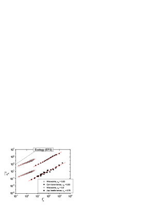
Figure 1: Fluctuation scaling for ensemble averages of the population of four species. Every point represents the mean $\overline{f_{A}}$ and variance $\overline{\sigma^{2}_{A}}$ over an ensemble of areas of the same size $A$ taylor . The bottom dashed line corresponds to $\alpha_{E}=1/2$, the top one to $\alpha_{E}=1$. Points were shifted both vertically and horizontally for better visibility.

II.2.3 Life sciences

There is a number of findings from cellular and molecular biology regarding FS. Azevedo and Leroi cells conducted a very extensive study of how the typical cell count of a species is related to its fluctuations from individual to individual. They found that FS holds over almost $10$ orders of magnitude in size, between more than $2000$ species, see Fig. 2. The exponent $\alpha_{\mathrm{E}}$ differs among tissue types, but for entire organisms its value is approximately $1$. Kendal kendal.tumor presents similar findings for the number of tumor cells in groups of mice, but the exponents vary.

Similarly, Kendal kendal.genomevar analyzed for the most common variations in the human genome called Single Nucleotide Polymorphisms (SNPs) genomevar . He found that the mean and the variance of the number of SNPs in a DNA sequence scale as different non-trivial powers of the length of the sequence, and thus the variance also scales with the mean.

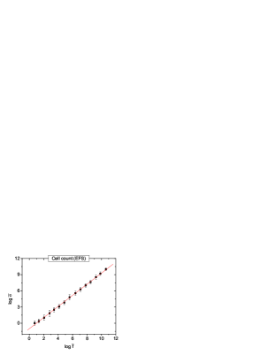
Figure 2: Fluctuation scaling for the cell count of species. For every species the average cell count $\overline{f}$ and its variance $\overline{\sigma^{2}}$ was calculated separately. Then these points were binned logarithmically for better visibility, error bars show the standard deviation of $\log\overline{\sigma}$ in the bins. $\alpha_{\mathrm{E}}=1$. Data courtesy of Ricardo Azevedo cells .

II.2.4 Physics

FS has been present in the physics literature as well. Many extensive quantities are known to have equilibrium fluctuations proportional to the square root of the system size, implying the value $\alpha_{\mathrm{E}}=1/2$ reichl ; landau5 . This relationship is a simple consequence of the central limit theorem (see Section III.2.1). Botet et al. botet.prl ; botet.pre ; botet.npb find EFS for a wide range of models, and also for the fragment multiplicity measured in heavy-ion collision experiments. Moreover, a linear ($\alpha=1$) relationship was found between the fluctuations and mean fluxes of cosmic radiation uttley.flux ; vaughan.flux . Here the ensemble is formed by cutting a single time series into pieces, and then periods with higher average activity exhibit higher fluctuations.

II.3 Empirical results: temporal averages

We will now turn to temporal FS. For the collection of such data it is necessary to have multi-channel measurements, simultaneously monitoring the behavior of a range of elements $i$. With the unbroken growth of computing infrastructure, many technological networks now offer appropriate datasets, several ones publicly available.

II.3.1 Complex networks

Menezes and Barabási barabasi.fluct ; barabasi.separating , in part inspired by Taylor’s original paper, found TFS for several complex networks. A good example is the analysis of Internet traffic, which was later revisited by Duch and Arenas duch.internet . In their study they analyzed the traffic of the Abilene backbone network. The nodes $i$ correspond to routers, and the mean and variance of their data flow was calculated. In Fig. 3 we show their results for weekly data traffic, the best fit is achieved with $\alpha_{\mathrm{T}}\approx 0.75$. Menezes and Barabási also analyzed web page visitations, river flow, microchip logical gates and highway traffic. They proposed that the datasets should fall into two "universality classes" with $\alpha_{\mathrm{T}}=1/2$ and $1$. There also exists a growing body of literature on transport processes on networks, and the scaling of fluctuations in such systems eisler.internal ; duch.internet ; menezes.flux ; tadic.loops ; duch.model .

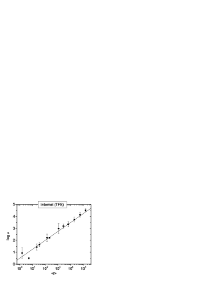
Figure 3: Fluctuation scaling for the traffic of Internet routers. For every router the temporal average of weekly data traffic $\left\langle f_{i}\right\rangle$ and its standard deviation $\sigma_{i}$ was calculated separately. Then these points were binned logarithmically for better visibility, error bars show the standard deviation of $\log\sigma$ in the bins. The fitted exponent is $\alpha_{\mathrm{T}}=0.75$. Data courtesy of Jordi Duch and Alex Arenas duch.internet .

II.3.2 Ecology

Ecologists have made many advances regarding TFS as well, but the literature is far from unequivocal. The basic concept is to monitor many populations of a given species for an extended period of time, and then for each population $i$ calculate the temporal mean $\left\langle f_{i}\right\rangle$ and standard deviation $\sigma_{i}$ of abundance. These are typically power law related according to TFS, examples are shown in Fig. 4.

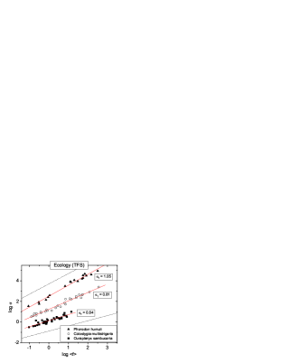
Figure 4: Fluctuation scaling for temporal averages of the population of three species. A point represents the temporal mean $\left\langle f_{i}\right\rangle$ and standard deviation $\sigma_{i}$ of a population. The bottom dashed line corresponds to $\alpha_{T}=1/2$, the top one to $\alpha_{T}=1$. Points were shifted both vertically for better visibility. Data courtesy of Marm Kilpatrick kilpatrick.ives ; taylor.insect .

Classical population dynamics offers several benchmark models may.complexity ; lotka ; volterra , but simple deterministic and Markovian models cannot explain the observed $\alpha_{\mathrm{T}}$ values between $1/2$ and $1$. After a range of small populations where they show realistic behavior, they cross over to either $\alpha_{\mathrm{T}}=1/2$ or $1$ keeling.simplestoch . The model of Kilpatrick and Ives kilpatrick.ives suggested that the interaction between species and feedback mechanisms between their fluctuations can give rise to any value of $\alpha_{\mathrm{T}}$. Perry proposed an even simpler chaotic model perry.chaotic . Both of these models can yield various exponents, but still only when populations are small enough.

There have been several findings for plant species. In a series of papers Ballantyne and Kerkhoff showed that the reproductive (yearly seed count) variability of trees follows TFS with $\alpha_{\mathrm{T}}=1$. The same value is supported by the Satake-Iwasa satake.iwasa forest model. There the trees are modeled by interacting oscillators which synchronize above a critical value of the coupling ballantyne.model ; ballantyne.correls . The synchronization transition coincides with a transition from $\alpha_{\mathrm{T}}=1/2$ to $\alpha_{\mathrm{T}}=1$.

We will now briefly describe their empirical study ballantyne.scaling . The dataset koenig.masting consists of yearly observations of the seed production of trees throughout the Northern Hemisphere. In particular, we considered three subsets of the dataset uponrequest , those collected by Tallqvist tallqvist , Franklin franklin and Weaver and Forcella weaver.forcella , including $4-17$ years of observations for $44$, $148$ and $28$ sites, respectively. The fits for TFS are given in Fig. 5(left). The exponents for the three subsets were found to be $\alpha_{\mathrm{T}}=0.97$, $0.93$ and $0.90$. Given the quality of the fits it is not possible to outrule that for all three datasets $\alpha_{\mathrm{T}}=1$ (as suggested by Ref. ballantyne.scaling ). However, here we make an attempt to give an argument that predicts otherwise and can be tested.

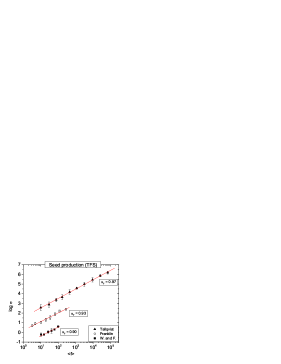
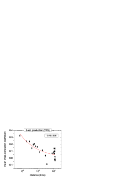
Figure 5: (left) Fluctuation scaling for the yearly seed count (reproductive activity) of trees from three studies. The fitted exponents are $\alpha_{\mathrm{T}}=0.90,0.93,0.97$. Points were logarithmically binned and $\log\sigma$ was averaged for better visibility, error bars show the standard deviation of $\log\sigma$ in the bins. The estimates are close to, but below $1$. (right) The average cross-correlation coefficient between pairs of sites as a function of their distance. Pairs of sites were binned to have an equal number per bin, error bars show the standard deviation of the cross correlation coefficients in the bins. The red line is a fit with the power law $C(r)\propto r^{-0.40}$, from the fit the error of the exponent is $\pm 0.06$.

Simulations of the Satake-Iwasa model already suggested that long-range synchronization can cause $\alpha_{\mathrm{T}}>1/2$, and the presence of such a tendency is well known for trees. Koenig and Knops koenig.masting conclude that there exists a significant positive correlation between the reproductive activity of trees for distances longer than $1000$ kms (this phenomenon is called masting in the ecology literature). While Ref. koenig.masting is much more precise and detailed, we also outline a simple measurement: in Fig. 5(right) we plot the average $C(r)$ cross-correlation coefficients between the sites in the complete dataset as a function of the distance $r$ of the sites. As expected, we find that cross-correlations decay very slowly with distance, and the dependence can be fitted approximately by

$$C(r)\propto r^{-0.40},$$ (6)

(although admittedly the fit is not perfect). Sections III.3.4 and IV.4 will show, that while perfect synchronization a’la Satake-Iwasa leads to $\alpha_{\mathrm{T}}=1$, partial synchronization with the above power-law correlations, implies $\alpha_{\mathrm{T}}=1-0.40/2=0.8$, see Eq. (20). A better quantitative agreement would warrant larger datasets which are not available at present, but there have been some promising attempts along the same lines ballantyne.correls .

II.3.3 Life sciences

Keeling and Grenfell measles suggested TFS for the size of epidemics, and found both empirically and by a simple Markov chain model of population dynamics that vaccination in general decreases not only the size of epidemics but also the value of $\alpha_{\mathrm{T}}$. TFS was later found by Woolhouse et al. pathogen to also hold between different pathogens. TFS has been found in the cell-to-cell variation of protein transcription by Bar-Even et al. bareven.protein , albeit with a crossover and a rather narrow range.

II.3.4 Stock market

In this section we summarize the results of a series of papers eisler.non-universality ; eisler.unified ; eisler.sizematters ; eisler.sizematters2 . The work was based on a TAQ database taq2000-2002 , recording the transactions of the New York Stock Exchange (NYSE) for the years $2000-2002$. Very similar results were obtained for the NASDAQ and Chinese markets jiang.fluxes .

We define the activity of stock $i$ as its total traded value, given as

$$f_{i}^{\Delta t}(t)=\sum_{n=1}^{N^{\Delta t}_{i}(t)}V^{\Delta t}_{i,n}(t),$$

where $N^{\Delta t}_{i}(t)$ is the number of transactions of stock $i$ in the period $[t,t+\Delta t)$. The individual values of these transactions are denoted by $V^{\Delta t}_{i,n}(t)$. Data were detrended by the well-known $U$-shaped daily pattern of traded volumes eisler.non-universality .

Then the measurement of mean and variance was carried out. The exponent $\alpha_{\mathrm{T}}$ shows a strong dependence on the window size $\Delta t$, we will return to this result in Section III.3.1. The values range between $\alpha_{\mathrm{T}}=0.68-0.87$, see Fig. 6.

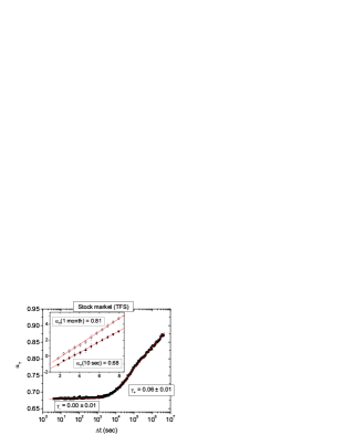
Figure 6: The dependence of the FS exponent in stock market data on the size of the time window $\Delta t$. The dependence is logarithmic in two regimes, with the coefficients $\gamma_{-}\approx 0.00$ for $\Delta t<10^{3}$ sec and $\gamma_{+}\approx 0.06$ for $\Delta t>3\times 10^{4}$ sec. The crossover regime corresponds to the time scale of one trading day. Inset: FS for the fluctuations of the traded value of stocks for the window sizes $\Delta t=10$ sec and $\Delta t=1$ month. Points were logarithmically binned and $\log\sigma$ was averaged for better visibility, error bars show the standard deviation of $\log\sigma$ in the bins.

When $\Delta t$ is very small, Ref. eisler.unified shows that the individual transactions can be treated as independent events. Moreover, for the large enough stocks the average size of transactions ($\left\langle V_{i}\right\rangle$) can be calculated as a power of the mean number of transactions as

$$\left\langle V_{i}\right\rangle\propto\left\langle N_{i}\right\rangle^{\beta},$$

with $\beta\approx 0.65$ eisler.unified . Equivalents of this property recur in several FS-related contexts. We will devote Sections III.3.2-III.3.3 to this observation, which we will call impact inhomogeneity eisler.unified . We will also show how to map the value of $\beta$ onto non-trivial $\alpha_{\mathrm{T}}$ values. By that method [see Eq. (18)] the corresponding $\alpha_{\mathrm{T}}$ value should be $0.70$, which is very close to the actual value $\alpha_{\mathrm{T}}(\Delta t\rightarrow 0)=0.69$.

Another general observation eisler.unified is that if $\alpha_{\mathrm{T}}$ is a function of $\Delta t$, then FS can only hold, if this dependence is logarithmic (cf. Section III.3.1). For the stock market this is true in two distinct regimes and those are separated by a crossover. For $\Delta t<10^{3}$ sec ($-$ sign) and $\Delta t>3\times 10^{4}$ sec ($+$ sign) one finds

$$\alpha_{T,\pm}(\Delta t)=\alpha^{*}_{T,\pm}+\gamma_{\pm}\log\Delta t,$$

with $\gamma_{-}\approx 0.00$, and $\gamma_{+}\approx 0.06$. On the other hand, the Hurst exponent $H_{i}$ can be defined as vicsek.book ; dfa

$$\sigma_{i}(\Delta t)=\left\langle\left[f_{i}^{\Delta t}(t)-\left\langle f_{i}^{\Delta t}(t)\right\rangle\right]^{2}\right\rangle^{1/2}\propto\Delta t^{H_{i}}.$$ (7)

For NYSE this equation is found to be valid with

$$H_{i;\pm}=H^{*}_{\pm}+\gamma_{\pm}\log\left\langle f_{i}\right\rangle.$$

Lower indices indicate the same two regimes, and $\gamma_{\pm}$ have the same values as for $\alpha_{T}$ eisler.unified .

Subj.	System	T/E	Refs.
Networks	Random walk	T	barabasi.fluct ; barabasi.separating ; eisler.internal
	Network models	T	tadic.loops ; menezes.flux
	Highway network	T	barabasi.fluct ; barabasi.separating
	World Wide Web	T	barabasi.fluct ; barabasi.separating
	Internet	T	barabasi.fluct ; barabasi.separating ; duch.internet
Phy.	Heavy ion collisions	E	botet.prl ; botet.pre ; botet.npb
	Cosmic rays	E	uttley.flux ; vaughan.flux
Soc./econ.	Stock market	T	eisler.non-universality ; eisler.unified ; eisler.sizematters ; jiang.fluxes
	Stock market	E	this review
	Business firm growth rates	E	stanley.firm ; amaral.growth
	Email traffic	T	this review
	Printing activity	T	this review
Cl.	River flow	T	janosi.danube ; dahlstedt.river
	Precipitation	T	eisler.inprep
Ecology/pop. dyn.	Forest reproductive rates	T	ballantyne.scaling ; ballantyne.correls
	Satake-Iwasa forest model	T	ballantyne.model
	Crop yield	T	fairfield.smith
	Animal populations	T, E	taylor ; anderson.variability ; conserv ; maurer.taper
	Diffusion Limited population	E	kendal.dla
	Population growth	T	keitt.pop ; keitt.scaling
	Exponential dispersion models	E	kendal.ecological ; kendal.blood ; kendal.tumor
	Interacting population model	T	kilpatrick.ives
Life sciences	Cell numbers	E	cells
	Protein expression	T	bareven.protein
	Gene expression	T	nacher.gene ; tadic.gene
	Individual health	E	mitninski.ageing
	Tumor cells	E	kendal.tumor
	Human genome	E	genomevar ; kendal.genomevar
	Blood flow	E	kendal.blood
	Oncology	E	kendal.tumor
	Epidemiology	T	measles ; pathogen

Table 2: A list of some studies where fluctuation scaling/Taylor’s law was directly applied or implied by a similar formalism. Groups were assigned by subject areas, Phy. = Physics, Cl. = Climatology. The column T/E shows the type of fluctuation scaling, T: temporal, E: ensemble.

II.4 New empirical results

In this section we present previously unpublished results for fluctuation scaling. Note that temporal variances were estimated by the partition function of Detrended Fluctuation Analysis dfa . This was necessary in order to (at least partly) remove the nonstationarity from the datasets. All results, including the values of $\alpha_{\mathrm{T}}$ agree qualitatively with those obtained from a direct calculation variance without detrending, but the accuracy of the estimation is improved.

II.4.1 Stock market (ensemble averaging)

Fluctuation scaling in stock market data has just been discussed, but those earlier results pertained temporal FS, whereas here we will present some new findings on ensemble FS in the same dataset.

We again consider the (daily) trading activity of stocks. The size of companies is often measured by the total value of all their issued stocks, called the company’s capitalization ($C$). We take a fixed time period, the day 03/01/2000 (the results are similar for other days). Then we group the stocks according their capitalization into $35$ logarithmic bins. Finally, we calculate the mean $\overline{f_{C}}$ and the standard deviation $\overline{\sigma_{C}}$ of the activity in every group. EFS is shown in Fig. 7. The fit gives $\alpha_{\mathrm{E}}\approx 0.8-0.9$, although with some deviations from scaling.

If the size of the animal population is extensive, it is justifiable to use the size of the area to parametrize the ensemble: its mean should be exactly proportional to the area. To use capitalization as a parametrization for company size is a different matter. While it is indeed strongly related to the mean trading activity, there is no one-to-one correspondence between the two eisler.sizematters . This means that companies of the same capitalization can have different expected trading activities. Thus our ensemble averaging technique is only approximate.

To circumvent this problem one can apply the following trick. The trading activity of companies fluctuates strongly from day to day, but the expectation value of the distribution is rather stable over time. So let us now take an interval $t=1\dots T$ and calculate the time averages $\left\langle f_{i}(t)\right\rangle$ during this period for each stock. Then for every stock take the single value $f_{i}(t=1)$ only, and group the observations according to $\left\langle f_{i}\right\rangle$. This is equivalent to the measurement before, only instead of $C_{i}$, groups are formed with respect to $\left\langle f_{i}\right\rangle$ ($15$ logarithmic bins). Then the ensemble mean $\overline{f}$ and variance $\overline{\sigma}$ can be calculated in each group. The results from this technique are also indicated in Fig. 7, one can see a dramatic decrease in the noise level, while the value of the exponent is approximately preserved, $\alpha_{\mathrm{E}}=0.89$.

It must be emphasized that we use information about the temporal average only for the grouping procedure. The measured $\alpha_{\mathrm{E}}$ is a true EFS exponent. Moreover, the value of $\alpha_{\mathrm{E}}$ that we find here is much larger than $\alpha_{\mathrm{T}}$ (cf. Section II.3.4). Because of the intricate statistical properties of markets, the two exponents cannot be expected to coincide.

This example shows that the success of ensemble fluctuation scaling crucially depends on the proper choice of the size parameter. In the cases where possible, physical size or area are good choices, because they are known to be extensive. Otherwise the above trick can be applied, but only if multiple observations are available for every node and the system is close to stationary.

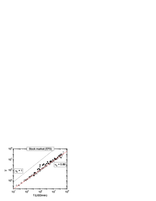
Figure 7: Fluctuation scaling considered as an ensemble average over NYSE stocks for the trading activity. Calculations were done both by considering the capitalization $C_{i}$ (03/01/2000: $\blacksquare$), and the monthly average trading activity $\left\langle f_{i}\right\rangle$ (03/01/2000: $\Circle$, 01/02/2000: $\bigtriangleup$, 01/03/2000: $\bigtriangledown$) as surrogates for size. One can see that using $\left\langle f_{i}\right\rangle$ for the formation of groups largely reduces fluctuations, but the exponent remains similar.

II.4.2 Human dynamics

The analysis of the records of human dynamics has recently seen growing interest barabasi.human ; barabasi.einstein ; vazquez.human . Here we discuss two large technological databases of human activity:

1. Emails from the employees of the company Enron during the year $2000$. We used a filtered variant of the original dataset posted by the Federal Energy Regulatory Commission enron.data . We defined $f_{i}^{\Delta t}(t)$ as the number of emails sent by the person $i$ during the interval $[t,t+\Delta t)$.

2. Data on the printing activity of the largest printer at the Department of Computing at Imperial College London print.data . The files include the complete year $2003$, we removed weekends, official holidays and closure times of the computer laboratory (23:00-7:00). We included $987$ users who submitted at least $3$ documents during our analysis, except the single largest user who appeared to have different statistical properties from the rest. $f_{i}(t)$ is defined as the number of documents submitted to print by user $i$ in the time interval $[t,t+\Delta t)$. Further details on the dataset can be found in Ref. paczuski.printing .

Note that multiple copies of the same email/document sent/submitted simultaneously were counted as one.

We are going to present these two datasets side by side, because they have strong similarities. Both show TFS for window sizes $\Delta t=5\dots 2.8\times 10^{4}$ sec. The exponent varies between $\alpha_{\mathrm{T}}=0.52-0.72$ (email) and $\alpha_{\mathrm{T}}=0.57-0.83$ (printing). Fig. 8 shows the fits for time window sizes $\Delta t=10,10000$ sec. We find scaling over about $2.5$ orders of magnitude, and the exponent depends on $\Delta t$, as shown in Fig. 9. Despite the level of the noise in the data, the dependence appears to be monotonically increasing, with two regimes separated by a crossover near $\Delta t\sim 4000$ sec (email) and $\Delta t\sim 1000$ sec (printing). The dependence is close to logarithmic, with the same form as for stock markets (the index $-$ corresponds to the regime below, $+$ above the crossover):

$$\alpha_{T,\pm}(\Delta t)=\alpha^{*}_{T,\pm}+\gamma_{\pm}\log\Delta t,$$

with $\gamma_{-}^{\mathrm{email}}\approx 0.04$, $\gamma_{+}^{\mathrm{email}}\approx 0.13$, $\gamma_{-}^{\mathrm{print}}\approx 0.09$, and $\gamma_{+}^{\mathrm{print}}\approx 0.02$. Also for the Hurst exponents

$$H_{i;\pm}=H^{*}_{\pm}+\gamma_{\pm}\log\left\langle f_{i}\right\rangle.$$

The coefficients are $\gamma_{-}^{\mathrm{email}}\approx 0.04$, $\gamma_{+}^{\mathrm{email}}\approx 0.11$, $\gamma_{-}^{\mathrm{print}}\approx 0.07$, and $\gamma_{+}^{\mathrm{print}}\approx 0.01$. The $\sigma_{i}(\Delta t)$ scaling plots are shown in Fig. 10, and the Hurst exponents’ dependence on $\left\langle f\right\rangle$ in Fig. 11.

Finally, notice that for email data $\alpha_{\mathrm{T}}(\Delta t)$ tends to $1/2$ with decreasing window size, and the logarithmic tendency appears to saturate. On the other hand, for printing data the logarithmic tendency is markedly present even for short times. By an extrapolation from the trend one expects that $\alpha_{\mathrm{T}}(1\ \mathrm{sec})\approx 0.51$. Section III.2.1 offers an explanation why for very short times one expects $\alpha_{\mathrm{T}}=1/2$ in these datasets.

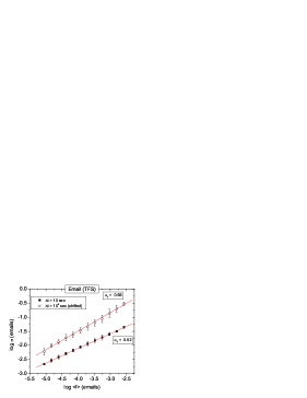
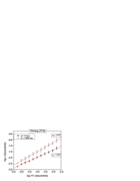
Figure 8: Fluctuation scaling for time resolutions of $\Delta t=10$ sec and $\Delta t=10000$ sec. Points were logarithmically binned and $\log\sigma$ was averaged for better visibility, the error bars represent the standard deviations inside the bins. (left) Results for the number of sent emails. (right) Results for number of printed documents.

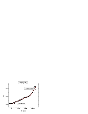
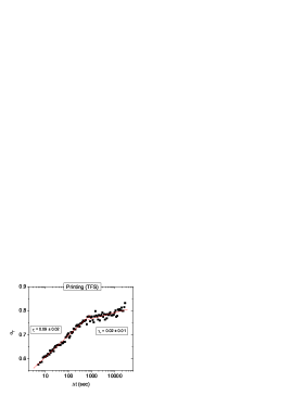
Figure 9: (left) The dependence of the FS exponent in the Enron email database on the size of the time window $\Delta t$. The dependence is logarithmic in two regimes, with the coefficients $\gamma_{-}\approx 0.04$ for $\Delta t<4000$ sec and $\gamma_{+}\approx 0.13$ for $\Delta t>4000$ sec. (right) The dependence of the FS exponent in printing data on the size of the time window $\Delta t$. The dependence is logarithmic in two regimes, with the coefficients $\gamma_{-}\approx 0.09$ for $\Delta t<300$ sec and $\gamma_{+}\approx 0.02$ for $\Delta t>1000$ sec.

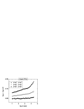
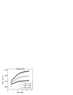
Figure 10: Scaling plots of $\log\sigma-1/2\times\log\Delta t$ versus $\log\Delta t$ generated by Detrended Fluctuation Analysis. Users were grouped by their average activity into three groups ($\left\langle f\right\rangle$ increasing from bottom to top, see plot for ranges) and the curves were averaged within groups. A horizontal line would correspond to complete the absence of correlations, and the slopes of the linear regimes are $H-0.5$, where $H$ are the typical Hurst exponents of groups. (left) Results for Enron email data. For shorter time windows $\Delta t<4000$ sec, correlations are weak, and their strength increases slowly with greater $\left\langle f\right\rangle$. Then after a crossover regime, for $\Delta t>4000$ sec correlations become stronger, with larger difference between the three groups. (right) Results for printing data. For shorter time windows $\Delta t<300$ sec, positive correlations exist, and their strength increases with greater $\left\langle f\right\rangle$. Then after a crossover regime, for $\Delta t>1000$ sec correlations become very weak for all three groups.

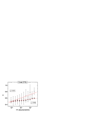
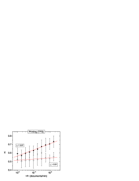
Figure 11: The dependence of the Hurst exponent of $f$ on $\left\langle f\right\rangle$. Points were logarithmically binned and $H$ was averaged for better visibility, the error bars represent the standard deviations inside the bins. (left) Results for Enron email data. When $\Delta t<4000$ sec ($\blacksquare$), depend weakly on $\left\langle f\right\rangle$, the coefficient of the logarithmic trend is $\gamma_{-}=0.04$, correlations are weak, $H_{i;-}\approx 0.5-0.55$. For time windows $\Delta t>4000$ sec ($\Circle$), correlations become stronger, $\gamma_{+}=0.11$, but there are strong fluctuations around the logarithmic trend. (right) Results for printing data. When $\Delta t<300$ sec ($\blacksquare$), the Hurst exponents depend logarithmically on $\left\langle f\right\rangle$ with a coefficient $\gamma_{-}=0.07$. For time windows $\Delta t>10^{3}$ sec ($\Circle$), correlations are nearly absent, the respective Hurst exponents are $H_{i;+}\approx 0.5-0.55$, and the logarithmic dependence is weak, with $\gamma_{+}=0.01$.

II.4.3 Precipitation

In this section we present a study eisler.inprep of the weekly precipitation records of $22928$ weather stations worldwide. The dataset was obtained from the Global Daily Climatology Network (GDCN) gdcn.data . For one station, typically $40$ years of data is available between $1950$ and $1990$. TFS is found with $\alpha_{\mathrm{T}}=0.77$, see Fig. 12. However, there are also some significant deviations. These can be interpreted based on geographical information: For every station, the geographical latitude ($l_{i}$, measured in degrees) and the height $h_{i}$ measured from sea level was known, and the multiple regression

$$\log\sigma_{i}=C+\alpha_{\mathrm{T}}\log\left\langle f_{i}\right\rangle+C_{l}|l_{i}|+C_{h}h_{i}+\epsilon_{i}$$ (8)

with an error term $\epsilon_{i}$ yields the results $C=0.896\pm 0.002$, $\alpha_{\mathrm{T}}=0.732\pm 0.002$, $C_{l}=-(8.79\pm 0.05)\times 10^{-3}$ and $C_{h}=(-6\pm 1)\times 10^{-6}$. All values are significantly different from zero at the $99.98\%$ confidence level. For the single parameter fit of TFS, $R^{2}=0.73$, while for the multiple regression (8) one finds $R^{2}=0.90$ which is a substantial improvement due to the inclusion of geogrephical latitude and, in smaller part, to the height above sea level. The remaining error term, although we did not find any appropriate explanatory variable, is still not unsystematic. By plotting $\epsilon_{i}$ on a map (see Fig. 13) one finds a strong geographical clustering with $\epsilon_{i}>0$ typically, but not exclusively, in continental areas. This systematic tendency suggests that a well-defined origin might exist for such corrections.

As for the value of $\alpha_{\mathrm{T}}$, its origin will be analyzed in a later study eisler.inprep . From preliminary studies it appears that it is not strongly dependent on the choice of the time scale $\Delta t$, and it is always significantly different from both $1/2$ and $1$.

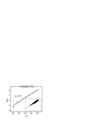
Figure 12: Fluctuation scaling for the weekly precipitation of weather stations. The fitted exponent is $\alpha_{\mathrm{T}}=0.77$. Points were logarithmically binned and $\log\sigma$ was averaged for better visibility, the error bars represent the standard deviations inside the bins. The inset shows the same plot and the same axis range, but without binning. One can see that there is a high number of outliers, due to other, $\left\langle f\right\rangle$-independent corrections to FS.

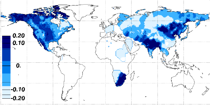
Figure 13: The error terms $\epsilon_{i}$ of the multiple regression (8), which represent the residuals of $\log\sigma$ after correcting for average precipitation, geographical latitude and height above sea level. $\epsilon_{i}$ accounts for $10\%$ of the variance in $\log\sigma_{i}$, and it is strongly clustered geographically suggesting the existence of a well-defined underlying mechanism.

II.5 Corrections to fluctuation scaling

Similarly to precipitation data, there are significant corrections to TFS also in stock markets. These are related to differences between market sectors. In Fig. 14 we plot $\sigma_{i}/\left\langle f_{i}\right\rangle^{\alpha_{\mathrm{T}}}$ versus $\left\langle f_{i}\right\rangle$ to characterize corrections to fluctuation scaling. By highlighting the alignment of three industrial sectors one can see that they form clusters, so the deviations are – to some degree – systematic.

In most real systems fluctuation scaling is found rather as a general tendency than an exact law. The scaling plots have some broadening, which can have several origins. A possible origin of poor fits can be the presence of crossovers and breaks in the scaling plots ballantyne.correls ; anderson.variability ; keeling.simplestoch ; barabasi.fluct , although these can only be seen clearly in very few studies botet.prl ; janosi.danube . In other cases the deviations are attributed to the quality of data and short sampling intervals smallsampletaylor . Still, these corrections can be large and systematic. In Section II.4.3 we showed that for precipitation fluctuations geographical location and height plays a role. Similarly, for the stock market the market sector matters. These effects could be uncovered, because of the availability of these independent quantities for each station/stock. In some models they can even be calculated analytically, see Section IV.1.2.

The fact that scaling is mostly very well preserved suggests that the investigated complex systems have a robust dynamics characterized by a value of $\alpha$, and that the role of the corrections is not substantial in the formation of fluctuations. There is wide consensus that the exponents are meaningful, and not significantly distorted by the non-scaling corrections.

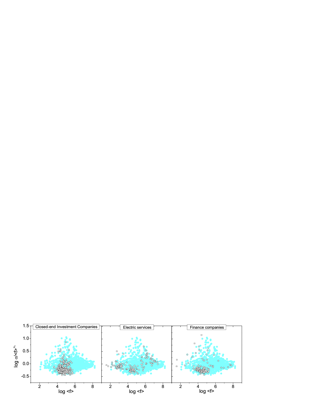
Figure 14: $\log[\sigma_{i}/\left\langle f_{i}\right\rangle^{\alpha_{\mathrm{T}}}]$ plotted versus $\log\left\langle f_{i}\right\rangle$ for the $10$-second resolution traded value data of stocks. The data points were not binned or altered in any way, which makes visible the deviations from the original scaling law, which would correspond to a horizontal line. The lighter points indicate all stocks, while boxes ($\Box$) highlight the distribution of points for the three indicated economic sectors. The great degree of clustering both horizontally and vertically. Clustering along the $\log\left\langle f\right\rangle$ axis only suggests that the sector has some typical trading activity. Systematic corrections to fluctuation scaling are indicated by clustering along the $\log\sigma/\left\langle f\right\rangle^{\alpha_{\mathrm{T}}}$ axis. If a sector is clustered in the lower/higher half of the dataset, it means that its trading activity has typically lower/higher fluctuations than the market average. The presence of such sector dependent clustering suggests that the corrections to fluctuation scaling are not purely random.

II.6 Summary of observations

In sum, fluctuation scaling appears to be a surprisingly general concept that can be recognized in virtually any discipline where the proper data are available. The fluctuations of positive additive quantities appear to have the structure

$$\mathrm{fluctuations}=\mathrm{const.}\times\mathrm{average}^{\alpha}\times(1+\mathrm{corrections}).$$

There is immense literature on the origins of fluctuations in various systems, ranging from gene networks paulsson.summing through complexity barabasi.separating to animal populations noisy.clockwork ; engen.demographic ; saether ; sheep . The common point of all these works is that fluctuations originate from two factors: internal and external. Naturally, the dynamics, the structure, and the interaction of the nodes vary from case to case. We expect that, e.g., the stock market trading activity and the reproduction of trees is very different. The discovery of FS as a common pattern can be a good start to point out further analogies and to build a broader picture.

III A general formalism

In the following we will focus on the temporal variant of FS. In many cases the results continue to apply by simply dropping the time index $t$ and averaging over an ensemble of systems.

The previous section reviewed ample evidence that FS emerges in a very broad range of areas. Here we attempt to describe many of these by the same formalism. In the following we will assume that the systems are stationary. When considering a node $i$, its activity $f_{i}$ will always be decomposed as a sum. In some cases this means summation over the node’s internal constituents, as for forests where reproductive activity was the total of that for all trees. In other cases the nodes themselves are simple, and the signal is the sum of events at the nodes, like the passing of cars at counting stations. If in the time interval $[t,t+\Delta t)$ there are $N_{i}^{\Delta t}(t)$ such constituents/events, and the activity of the $n$’th contributes $V_{i,n}^{\Delta t}(t)$ to the total activity $f_{i}$, then

$$f_{i}^{\Delta t}(t)=\sum_{n=1}^{N_{i}^{\Delta t}(t)}V^{\Delta t}_{i,n}(t).$$ (1)

These $V$’s do not necessarily have to be independent ballantyne.correls ; eisler.unified , but we will assume that their (unconditional) distribution does not depend on $n$. We will omit the index $\Delta t$, where appropriate.

III.1 The components of fluctuations

Throughout this section we will analyze the fluctuations of quantities of the form (1), as measured by the standard deviation/variance. Thus, it is important that there exists a simple analytical expression eisler.sizematters2 for

$$\sigma^{2}_{i}=\left\langle\left[f_{i}(t)-\left\langle f_{i}(t)\right\rangle\right]^{2}\right\rangle.$$

Appendix A gives a proof that

$$\sigma^{2}_{i}=\Sigma^{2}_{Vi}\left\langle N_{i}^{2H_{Vi}}\right\rangle+\Sigma^{2}_{Ni}\left\langle V_{i}\right\rangle^{2},$$ (9)

where $\left\langle V_{i}\right\rangle$ and $\Sigma^{2}_{Vi}$ are the mean and the variance of $V_{i,n}$. Similarly, $\left\langle N_{i}\right\rangle$ and $\Sigma^{2}_{Ni}$ are the mean and variance of $N_{i}$. We also introduced the Hurst exponent $H_{Vi}$ of the constituents, which is defined as

$$\Sigma^{2}_{Vi}(N)=\left\langle\left[\sum_{n=1}^{N}V_{i,n}-\left\langle\sum_{n=1}^{N}V_{i,n}\right\rangle\right]^{2}\right\rangle\propto N^{2H_{Vi}}$$ (10)

for any $t$ and $\Delta t$. If for a fixed $i$ and $t$ all $V_{i,n}(t)$ are uncorrelated, then $H_{V}=1/2$, while if they are long range correlated $H_{V}>1/2$ hurst ; dfa .

III.2 "Universality" classes

In this formalism it is relatively easy to show that there exist two important classes of systems, one with $\alpha=1/2$ and one with $\alpha=1$. The existence of such classes was pointed out, for example, by Anderson et al. anderson.variability and later by Menezes and Barabási barabasi.fluct .

These are not universality classes but rather simple limiting cases, and $\alpha$ is not a universal exponent in the usual sense of statistical physics reichl . Many empirical systems do not belong to either class, and both $\alpha=1/2$ and $\alpha=1$ can arise from several types of dynamics. In order to make FS a truly useful tool in the analysis of empirical data, one needs a classification scheme for how different types of dynamics can be mapped onto $\alpha$. Our current understanding of such classification is outlined in this section.

III.2.1 The case $\alpha=1/2$

We will now present two scenarios that can give rise to $\alpha=1/2$. The arguments will be given in the language of time averages, but they can be generalized to ensemble averages in a straightforward way.

1. Let us assume that every node $i$ consists of a fixed number $N_{i}(t)=N_{i}$ of constituents, each with a signal $V_{i,n}(t)$ which is i.i.d. for all $i$, $n$ and $t$, with the same mean $\left\langle V\right\rangle$ and variance $\Sigma^{2}_{V}$. From Eq. (9) it is trivial that here $\sigma^{2}_{i}=N_{i}\Sigma^{2}_{V}.$ Because of the linearity of the mean, $\left\langle f_{i}\right\rangle=N_{i}\left\langle V\right\rangle,$ so

   $$\sigma^{2}_{i}=\frac{\Sigma^{2}_{V}}{\left\langle V\right\rangle}\left\langle f_{i}\right\rangle,$$

   and hence $\alpha=1/2$. Of course in this simple case one can say more, because the central limit theorem feller is applicable:

   $$\frac{\sum_{n=1}^{N_{i}}V_{i,n}(t)-N_{i}\left\langle V\right\rangle}{\sqrt{N_{i}}\Sigma_{V}}\rightarrow\mathcal{G}_{i}(t),$$ (11)

   where $\mathcal{G}_{i}(t)$ are i.i.d. standard Gaussians and "$\rightarrow$" means convergence in distribution for $N_{i}\rightarrow\infty$.

   Exactly the same equation can be rewritten to more resemble fluctuation scaling:

   $$\frac{f_{i}(t)-\left\langle f_{i}\right\rangle}{K\left\langle f_{i}\right\rangle^{\alpha}}\rightarrow\mathcal{G}_{i}(t).$$ (12)

   The power $\alpha=1/2$ is exactly the power in FS, and $K=\Sigma_{V}\left\langle V\right\rangle^{-1/2}$. The conceptual difference is only that since we know that $\left\langle f_{i}\right\rangle=N_{i}\left\langle V\right\rangle$, we can use $\left\langle f_{i}\right\rangle\left\langle V\right\rangle^{-1}$ as a surrogate variable for $N_{i}$. This is very useful, when we only have the time series of $f_{i}(t)$ available but not $N$, since the limit can be switched to $\left\langle f\right\rangle\rightarrow\infty$ (cf. Section V.2).

2. Let us consider an example for scenario 1): a system, where $V_{i,n}(t)$ can only be $1$ with probability $p$ and $0$ with probability $1-p$. Scenario 1) still applies because $V$’s are i.i.d., so $\alpha=1/2$. This binary distribution can be instructive, as one can think of $V_{i,n}(t)$ as independent indicator variables. For example let us take a volume $S$ of ideal gas within a large container. Let the whole system contain $N$ gas atoms, and $V_{i,n}=1$ if the $n$’th atom is in the container, while $V_{i,n}=0$ if it is not. The ideal gas is homogeneous and the atoms are independent, every atom having a probability $p\propto S$ of being in the small container. From here, one can apply the above argument to show that for various containers of different sizes

   $$\sigma_{S}\propto\left\langle f_{S}\right\rangle^{1/2}.$$

   These are the well-known square-root type fluctuations of equilibrium statistical physics (see, e.g., Section XII of Ref. landau5 ). Similar arguments were suggested for the number of animals in an area: If the motion of individuals were independent (gas-like), then their spatial density fluctuations should follow $\alpha=1/2$ taylor.woiwod .

3. The example of the ideal gas can be given in the language of ensemble averages as well. Simply we take a large number of containers of the same size $S$ and calculate the mean $\overline{f_{S}}$ and standard deviation $\overline{\sigma_{S}}$ of atom counts between these containers. Then we vary the container size, and we recover an analogous relationship:

   $$\overline{\sigma_{S}}\propto\overline{f_{S}}^{1/2}.$$

   Of course, this was expected, because the system is ergodic, so temporal and ensemble averages are equal.

4. For an even simpler mechanism let us recall the findings of Section II.4.2. We found that for very short times ($\Delta t\sim 1$ sec) the number of sent emails/printed documents follow TFS with $\alpha_{\mathrm{T}}=1/2$. It is highly unlikely that someone will send several different emails/print several different documents in the same second (duplicates of the same email to multiple recipients were excluded). Thus $f_{i}(t)=0$ or $1$, and so $f_{i}(t)=f_{i}^{2}(t)$. Remember that this is very different from the previous example, where $f_{i}(t)$ was allowed to have any value, and only $V_{i,n}(t)$’s were constrained to $0$ or $1$.

   In the email/print data the number of events per second was very low, generally $\left\langle f_{i}\right\rangle<4\times 10^{-3}$ sec^-1. The standard deviation is then

   $$\sigma_{i}^{2}=\left\langle f_{i}^{2}\right\rangle-\left\langle f_{i}\right\rangle^{2}=\left\langle f_{i}\right\rangle-\left\langle f_{i}\right\rangle^{2}\approx\left\langle f_{i}\right\rangle,$$ (13)

   so $\alpha=1/2$. The same argument holds for the number of trades per second in the stock market eisler.unified .

   The meaning of this scenario 2) in summary: We are examining the system on such a short time scale that no two events happen in the same time window. Then, the FS exponent tells us nothing about the dynamics of the system, because $\alpha=1/2$ is automatically true.

III.2.2 The case $\alpha=1$

We will now present two scenarios that can give rise to the value $\alpha=1$. While 1) is only valid for TFS, 2) can be readily generalized for EFS as well.

1. It was possible to obtain $\alpha=1/2$ by sums of independent $V$’s. In the other extreme case, if every node $i$ had a fixed number of identical and completely synchronized constituents, i.e., $N_{i}(t)=N_{i}$ and $V_{i,n}(t)\equiv V_{i}(t)$ Eq. (1) simplifies to

   $$f_{i}(t)=\sum_{n=1}^{N_{i}}V_{i,n}(t)=N_{i}V_{i}(t).$$

   Then $\left\langle f_{i}(t)\right\rangle=N_{i}\left\langle V_{i}(t)\right\rangle$, and $\sigma_{i}=N_{i}\Sigma_{Vi}$.

   $$\sigma_{i}=\frac{\Sigma_{Vi}}{\left\langle V_{i}\right\rangle}\left\langle f_{i}\right\rangle\propto\left\langle f_{i}\right\rangle^{\alpha},$$ (14)

   with $\alpha=1$. The last proportionality only holds if the ratio ${\Sigma_{Vi}}/{\left\langle V_{i}\right\rangle}$ is the same for any $i$, for example when the distribution of $V_{i}$ is independent of $i$.

2. How is such an argument of any use? The study of Cho et al. cho.genome reports experimental data on samples of yeast, in which cells were artifically prepared to have almost perfectly synchronized cell cycles. The measured signal $f_{i}(t)$ is the hourly expression level of various genes $i$ in a sample. If all cells of yeast contribute in the same way to the measured expression level, and they are synchronized, then the value $\alpha_{\mathrm{T}}=1$ is simply an indicator of such a synchrony. Thus FS probably tells us nothing about the dynamics of gene transcription, and the exponent is simply due to the sample preparation.

   Nacher et al. nacher.gene propose a stochastic differential equation model that predicts the same exponent $\alpha_{\mathrm{T}}=1$ for this dataset ($\alpha_{\mathrm{T}}=1$ is confirmed by Ziković et al. tadic.gene ). They argue that self-affine temporal correlations are the origin of such a value. Section III.3.1 will show that self-affine temporal correlations do not contribute to $\alpha_{\mathrm{T}}$ in this way. Instead, our above explanation is simpler, and it suggests that the dataset cannot be used in favor of any proposed model based on the value of $\alpha_{\mathrm{T}}$.

3. Real systems are often not closed, but subject to outside forces. In certain cases this driving can be so strong that it can overwhelm the internal dynamics. If the internal structure of the system becomes irrelevant, this must also have an effect on FS. There have been a number of studies discussing how fluctuations in complex systems are formed as the sum of internally generated and externally imposed factors paulsson.summing ; noisy.clockwork ; engen.demographic ; saether ; sheep . Anderson et al. anderson.variability and Menezes and Barabási barabasi.fluct ; barabasi.separating suggested that $\alpha_{\mathrm{T}}=1$ can arise when the external driving force imposes strong fluctuations in either $V_{i}(t)$ or $N_{i}(t)$ (cf. Ref. noisy.clockwork ).

   When all $V_{i,n}(t)$ (the signals of every constituent at every node) become synchronized, then we are back at scenario 1): $\alpha=1$, because $f_{i}(t)/\left\langle f_{i}\right\rangle=V(t)/\left\langle V\right\rangle$ which has a universal, $i$-independent distribution.

   It is also possible that an external force $W(t)$ affects the number of constituents in the elements so strongly that the fluctuations of $N_{i}(t)$ become proportional only to this force. In this case $N_{i}(t)=A_{i}W(t)$, where $A_{i}$ are node-dependent constants. One expects that generally $\left\langle f_{i}(t)\right\rangle=A_{i}\left\langle W(t)\right\rangle\left\langle V_{i}\right\rangle$, whereas

   $$\sigma_{i}^{2}=\Sigma^{2}_{Ni}\left\langle V_{i}\right\rangle^{2}+\Sigma^{2}_{Vi}\left\langle N\right\rangle=A_{i}^{2}\Sigma^{2}_{W}\left\langle V_{i}\right\rangle+\Sigma^{2}_{Vi}A_{i}\left\langle W\right\rangle.$$

   If fluctuations in $W$ are so large that $\left\langle W\right\rangle\ll\Sigma_{W}^{2}$, then only the first term remains. After some algebraic steps

   $$\sigma_{i}^{2}\approx\frac{\Sigma^{2}_{W}}{\left\langle W\right\rangle^{2}\left\langle V_{i}\right\rangle}\left\langle f_{i}\right\rangle^{2}\propto\left\langle f_{i}\right\rangle^{2\alpha_{\mathrm{T}}},$$

   with $\alpha_{\mathrm{T}}=1$. The last proportionality is true if the distribution of $V_{i,n}$ does not depend strongly on $i$.

4. $\alpha=1$ can be a sign of a universal distribution of $f_{i}(t)/\left\langle f_{i}\right\rangle$, which only varies by a constant multiplicative factor throughout nodes. If this is true, then $f_{i}(t)$ can be decomposed into this factor $F_{i}$, and the universal random variable $V_{i}(t)$, which are identically distributed for all $i$. Naturally $\left\langle f_{i}\right\rangle=F_{i}\left\langle V\right\rangle$, and $\sigma^{2}_{i}=F_{i}^{2}\Sigma^{2}_{V}$, and $\sigma_{i}=\Sigma_{V}\left\langle V\right\rangle^{-1}\left\langle f_{i}\right\rangle$.

III.3 Other values of $\alpha$

It has been observed that many real systems obey FS with $\alpha$ values that significantly differ from both $1/2$ and $1$. In this section we summarize the current knowledge of general mechanisms that can give rise to intermediate values.

III.3.1 The dependence of $\alpha$ on the time resolution $\Delta t$

First of all, $\alpha$ can depend on the size of the time window used for its measurement. This phenomenological picture can be used to understand the results of Section II.3.4 for stock market trading, and Section II.4.2 for human activity.

Let us assume, that the activity time series are long time correlated with Hurst exponents $H_{i}$ that are allowed to depend on the node $i$. The Hurst exponent of the time series $f_{i}^{\Delta t}(t)$ was previously defined as

$$\sigma_{i}(\Delta t)=\left\langle\left[f_{i}^{\Delta t}(t)-\left\langle f_{i}^{\Delta t}(t)\right\rangle\right]^{2}\right\rangle^{1/2}\propto\Delta t^{H_{i}}.$$ (7)

This definition is almost exactly the same as Eq. (10) for $H_{V}$, the only difference being that now instead of the $N$ number of constituents we consider the time window size $\Delta t$ as the scaling variable. TFS deals with how the variance scales when one moves to stronger (larger $\left\langle f\right\rangle$) signals:

$$\sigma_{i}\propto\left\langle f_{i}\right\rangle^{\alpha}.$$ (3)

Eq. (7) takes an alternative point of view and suggests that for a fixed signal, in the presence of long-range temporal correlations, the variance can grow anomalously also by changing the time window.

Following Ref. eisler.unified , from Eqs. (7) and (3), it is easy to see that the roles of $\left\langle f_{i}\right\rangle$ and $\Delta t$ are analogous. Since the left hand sides are the same, one can write a third proportionality between the right hand sides:

$$\Delta t^{H_{i}}\propto\left\langle f_{i}\right\rangle^{\alpha(\Delta t)}.$$

After taking logarithm on both sides, and differentiating by $\partial^{2}/\partial(\log\Delta t)\partial(\log\left\langle f_{i}\right\rangle)$, one finds that asymptotically

$$\frac{dH_{i}}{d(\log\left\langle f_{i}\right\rangle)}\sim\frac{d\alpha(\Delta t)}{d(\log\Delta t)}\sim\gamma.$$ (15)

This means that both partial derivatives have the same constant value, which we will denote by $\gamma$.

Eisler and Kertész eisler.unified outline three scenarios for this equality to hold:

1. In systems, where $\gamma=0$, the exponent $\alpha$, is independent of window size, and the degree of temporal correlations ($H$) is the same at all nodes.

2. When $\gamma>0$, $\alpha(\Delta t)$ depends on $\Delta t$ logarithmically: $\alpha(\Delta t)=\alpha^{*}+\gamma_{1}\log\Delta t$. The Hurst exponent of the node also depends on $\left\langle f\right\rangle$ logarithmically with the same prefactor: $H_{i}=H^{*}+\gamma\log\left\langle f_{i}\right\rangle$.

3. It is possible that Eq. (15) only holds piecewise, for certain ranges in $\Delta t$. Two regimes are then separated by a crossover between two distinct values $\gamma_{\pm}$, and nodes will have separate Hurst exponents $H_{-}(i)$ and $H_{+}(i)$ in the two regimes.

Case (III) was shown for the stock market and human dynamics in Section II.3.

III.3.2 Impact inhomogeneity

Any value of $\alpha$ can easily arise without dependence on the time window. To better understand the reason how, consider three toy systems with the following elements.

1. Let us take a fair coin with $0$ written on one side and $1$ on the other, this will be our group $i=1$. Then take two such coins for group $i=2$, three for $i=3$, etc. In every time step we flip all coins in every group, and let $f_{i}$ equal the sum of the numbers we flipped in element $i$. Naturally $\left\langle f_{i}\right\rangle\propto i$ and, if all coins are independent, $\sigma_{i}\propto i^{1/2}$. Thus, for such a case $\alpha=1/2$.

2. Now let us take another fair coin with $0$ written on one side and $1$ on the other, this will be our element $i=1$. For $i=2$, we again take only one coin with sides $0$ and $2$. For any $i$, there will be a single coin with sides $0$ and $i$. Trivially $\left\langle f_{i}\right\rangle\propto i$, but also $\sigma_{i}\propto i$. So this time $\alpha=1$.

3. In our final example, let us mix the above two. For the $i$’th group there are $i$ coins, each having a side with $0$ and a side with $i$. Then $\left\langle f_{i}\right\rangle\propto i^{2}$, whereas $\sigma_{i}\propto i^{1/2}\times i$. We have just constructed a case for $\alpha=3/4$.

One can unify these examples by introducing impact inhomogeneity. One can write the contribution (impact) of the constituents at a node $i$ as

$$V_{i,n}(t)=\left\langle V_{i,n}\right\rangle\cdot X_{i,n}(t),$$ (16)

all $X_{n,i}(t)$ are i.i.d. with unit mean. We then allow $\left\langle V_{i,n}\right\rangle$ to depend on $\left\langle N_{i}\right\rangle$ as a power law between nodes eisler.internal ; keitt.scaling :

$$\left\langle V_{i,n}\right\rangle\propto\left\langle N_{i}\right\rangle^{\beta}.$$ (17)

According to Eq. (9) fluctuations can be calculated as

$$\sigma^{2}_{i}=\Sigma^{2}_{Vi}\left\langle N_{i}\right\rangle+\Sigma^{2}_{Ni}\left\langle V_{i}\right\rangle^{2}=$$

$$\Sigma^{2}_{X}\left\langle V_{i}\right\rangle^{2}\left\langle N_{i}\right\rangle+\left\langle N_{i}\right\rangle\left\langle V_{i}\right\rangle^{2}\propto\left\langle f_{i}\right\rangle^{2\alpha},$$

where $\Sigma^{2}_{X}=\left\langle X^{2}\right\rangle-\left\langle X\right\rangle^{2}$, and

$$\alpha=\frac{1}{2}\left(1+\frac{\beta}{\beta+1}\right),$$ (18)

where we introduced the new parameter $\beta$.

As a quick check, the three toy models correspond to $\beta=0$, $\alpha=1/2$ (all coins $0$ or $1$); $\beta=1$, $\alpha=3/4$ (the coins value proportional to their number) and $\beta\rightarrow\infty$, $\alpha=1$ (only one coin with growing value). There is always some $\beta\geq 0$ that allows us to reproduce a given value $\alpha\in[1/2,1)$, whereas the range $\beta<0$ covers all possibilities of $\alpha<1/2$ and $\alpha>1$.

III.3.3 Examples of impact inhomogeneity

The ecology literature has documented gaston.lawton ; gaston.range that empirically there is a strong positive correlation between the typical size of subpopulations ($\left\langle V\right\rangle$) and the number of subpopulations per unit area ($\left\langle N\right\rangle$) or the total population per unit area ($\left\langle f\right\rangle$). The conjecture that these quantities might behave as powers of each other as in Eq. (17) was proposed by Keitt et al. keitt.scaling , both across species and for individual subpopulations of the same species.

Kendal makes a similar suggestion, and shows that it generates non-trivial exponents in EFS for ecological populations kendal.ecological and the heterogeneity of blood flow in organs kendal.blood . In fact he does not point out the general mechanism, but instead refers to non-trivial EFS exponents as the property of a class of models, which entail impact inhomogeneity. Here we will omit most of the formalism; a proof that Kendal’s approach has impact inhomogeneity can be found in Appendix B.

Let us take the case of animal populations as the example. Kendal proposes that EFS holds with an exponent $1/2<\alpha<1$ if the population of an area can be described by the so-called Tweedie exponential dispersion models penis . These assume that (i) an area $i$ contains a Poisson distributed number of animal clusters ($N_{i}$), (ii) the size of individual clusters ($V_{i,n}$) is i.i.d. gamma distributed, (iii) and there is a power law relationship between the means of these two quantities. Of course, (iii) is the same as Eq. (17), along with all of its consequences.

As for blood flow kendal.blood , it is measured by the entrapment of radioactive microspheres in capillaries. In a fixed mass of tissue, the number of entrapment sites $N$ is assumed to be Poisson distributed, while the blood flow $V$ of the sites is taken as gamma distributed, along the same lines and with the same conclusions as above.

Finally, Section II.3.4 suggested impact inhomogeneity also as the origin of non-trivial FS exponents for the traded value on stock markets.

III.3.4 Constituent correlations

There exists a further mechanism to produce any value $1/2\leq\alpha\leq 1$, without considering the scaling property of impacts. The total output of node $i$ is given by the equation

$$f_{i}(t)=\sum_{i=1}^{N_{i}}V_{i,n}(t).$$ (1)

We also fix $N_{i}$ as time independent. If we assume that the unconditional distribution of $V$’s is independent from $N_{i}$, and also from $n$, then one can denote the expectation value $\left\langle V\right\rangle=\left\langle V_{i,n}(t)\right\rangle$.

The central idea is the introduction of correlations between constituents, i.e., variables with different $n$. Let us assume for simplicity that the elements are situated on a one-dimensional lattice, and their activity is long-range correlated in space, so that the correlation function decays as a power law,

$$C(\Delta n)\propto\left\langle V_{i,n}V_{i,n+\Delta n}\right\rangle-\left\langle V_{i,n}\right\rangle^{2}\propto\Delta n^{2H_{V}-2}.$$ (19)

$H_{V}$ is the same Hurst exponent, as defined in Eq. (10). Then, positively correlated patterns display $H_{V}>1/2$, for uncorrelated (or short range correlated) patterns $H_{V}=1/2$, and for anticorrelated (antipersistent) patterns $H_{V}<1/2$.

It follows from Eq. (9) that the fluctuation of the combined activity of all constituents is:

$$\sigma^{2}_{i}=\Sigma^{2}_{V}N_{i}^{2H_{V}}\propto\left\langle f_{i}\right\rangle^{\alpha},$$

where

$$\alpha=H_{V}.$$ (20)

This idea was (to our knowledge) first presented by West west.comments , and demonstrated on surrogate data sets, but it was not applied directly to any new problem. The role of spatial correlations in the formation of FS in the context of ecology was also suggested by Colman et al. colman.regulated and Ballantyne and Kerkhoff ballantyne.correls more recently. The idea is confirmed by simulations, see Section IV.4.

IV Models

In this section, we will discuss some models that can be used to understand basic facts about fluctuation scaling, how it arises and what its limitations are.

IV.1 Random walks on complex networks

IV.1.1 The model

It was proposed by Menezes and Barabási barabasi.fluct that random walks can generate TFS in the following way. Let us take a scale free Barabási-Albert network of $M$ nodes barabasi.rmp . We distribute $W$ independent random walkers (tokens) randomly to the nodes. Then, in every time step these jump from their current node to one of their neighbors randomly. The process is repeated for $s=1\dots s_{\mathrm{max}}$ steps, then it is halted and the total number of visits to each node $i$ is counted. This number defines $f_{i}(t=1)$. Then the deposition and the walk is repeated, up to $T$ times, giving the time series $f_{i}(t)$. We ran simulations with the parameters $M=20000$, $W=100$, $s_{\mathrm{max}}=100$ and $T=10000$.

One finds that TFS holds with an exponent $\alpha_{\mathrm{T}}=1/2$, see Fig. 15. This value is the same as what arises from sums of independent random variables, so the central limit theorem is a possible origin of FS for random walks. The next part presents an analytical calculation that confirms this conjecture.

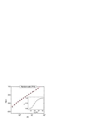
Figure 15: Fluctuation scaling for the random walker model on the Barabási-Albert network with parameters $M=20000$, $W=100$, $s_{\mathrm{max}}=100$ and $T=10000$. The fitted exponent is $\alpha_{\mathrm{T}}=1/2$ with a little deviation for very small $\left\langle f\right\rangle$. Points were logarithmically binned and $\log\sigma$ was averaged for better visibility, the error bars represent the standard deviations inside the bins. The inset shows the values of the effective exponents as one increases the fluctuations ($\Sigma_{W}$) in the number of walkers. There is a clear crossover from $\alpha_{\mathrm{T}}=1/2$ to $\alpha_{\mathrm{T}}=1$.

IV.1.2 Fluctuation scaling and corrections

The model can be solved based on a master-equation approach weiss.rw ; eisler.internal . Here we will use elementary probability theory instead. The number of walkers on node $i$ can be calculated from their distribution in the previous time step as:

$$N_{i}(s+1)=\sum_{j\in\mathcal{K}_{i}}\sum_{n=1}^{N_{j}(s)}\delta_{n}(j\rightarrow i;s),$$ (21)

where $\delta_{n}(j\rightarrow i;s)$ is a variable that is $1$ if in step $s$ the $n$’th token was at node $j$ and then it jumped to node $i$ (happens with probability $1/k_{j}$ to all neighbors of node $i$), and $0$ otherwise. $k_{i}$ is the degree of node $i$, $\mathcal{K}_{i}$ is the set of neighbors of node $i$, and $N_{j}(s=0)$ corresponds to the initial condition.

Calculations in Appendix C show that for such a model

$$\left\langle f_{i}\right\rangle=s_{\mathrm{max}}\left\langle N_{i}\right\rangle=k_{i}\frac{s_{\mathrm{max}}W}{\sum_{j}k_{j}}=\rho k_{i},$$ (22)

where $\rho=s_{\mathrm{max}}W/\sum_{j}k_{j}$. As the $W$ number of walkers is multiplied by the $s_{\mathrm{max}}$ and divided by the total number of edges, $\rho$ can be understood as the mean number of walkers passing any edge during the $s_{\mathrm{max}}$ time steps. Furthermore,

$$\sigma_{i}^{2}=\sum_{j\in\mathcal{K}_{i}}\frac{\sigma_{j}^{2}}{k_{j}^{2}}+\left\langle f_{i}\right\rangle.$$ (23)

The first term on the right hand side is a sum over $k_{i}$ nodes, but every term is multiplied by $1/k_{j}^{2}$, thus they can be neglected to a first order. To a leading order

$$\sigma_{i}^{2}=\left\langle f_{i}\right\rangle,$$

thus we find FS with $\alpha_{\mathrm{T}}=1/2$.

The term with the sum presents corrections to the scaling law. Eqs. (22) and (23) could be solved numerically, but to get a qualitative understanding of these corrections it is enough to make a self-consistent solution up to the first non-trivial order. This can be done by taking $\sigma_{j}^{2}=\left\langle f_{j}\right\rangle=\rho k_{j}$, and substituting it back into the right hand side of (23), to find

$$\sigma_{i}^{2}=\sum_{j\in\mathcal{K}_{i}}\frac{\rho}{k_{j}}+\rho k_{i}=\underbrace{\rho k_{i}}_{\left\langle f_{i}\right\rangle}\left(1+a\left\langle\frac{1}{k_{Ni}}\right\rangle\right),$$ (24)

where $\left\langle 1/k_{Ni}\right\rangle$ is the average inverse neighbor degree of node $i$ and $a=1$. Simulation results supporting this argument are shown in Fig. 16. We find that this formula accounts for a large part of the corrections to FS, only the coefficient is different, $a\approx 3.6$.

The qualitative picture from the above three equations is the following. For simplicity let us consider $\rho=1$, when the average number of tokens at a node equals its degree. Thus on average in every step every node transmits one token on each of its edges to its neighbors. Consequently every node receives typically one token on each edge, so again it will have tokens equal to its degree. These tokens arrive independently, thus the variance is proportional to their number, which implies $\alpha_{\mathrm{T}}=1/2$. The corrections in Eq. (24) imply that nodes with relatively higher degree neighbors (smaller $\left\langle 1/k_{Ni}\right\rangle$) exhibit lower fluctuations. This is because the number of tokens at a neighboring site with smaller degree is smaller, and thus can have larger relative fluctuations. These fluctuations then affect our site via a stronger variation in incoming tokens.

This argument is important, because it tells us that for random walks fluctuation scaling is only approximately true. The local topology of the network can give significant corrections which cause a broadening in the scaling plots and which are not simply due to measurement noise. According to Eq. (24) the size of the correction term depends on the neighborhood of the node. Because $\left\langle f_{i}\right\rangle\propto k_{i}$, very large flux nodes also have many neighbors. In an uncorrelated network the term $\left\langle 1/k_{Ni}\right\rangle$ will converge to a constant value with growing $k_{i}$, its node dependence (and thus the broadening it causes) is diminished.

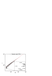
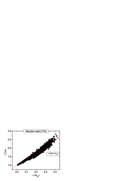
Figure 16: (left) Fluctuation scaling for the random walker model with parameters $M=20000$, $W=100$, $s_{\mathrm{max}}=100$ and $T=10000$. The same as Fig. 15, only without the binning procedure. The scaling law with $\alpha_{\mathrm{T}}=1/2$ holds on average, but there is some systematic broadening. The inset shows $10$ randomly selected points from the indicated area, with the average inverse neighbor degree $\left\langle 1/k_{Ni}\right\rangle$ indicated for each node. There is a general increasing tendency in $\left\langle 1/k_{Ni}\right\rangle$ from bottom to top. (right) The value of $\sigma/\left\langle f\right\rangle^{1/2}$ plotted versus the average inverse neighbor degree $\left\langle 1/k_{Ni}\right\rangle$ of the node. There is an approximately linear relationship of the form $\sigma^{2}/\left\langle f\right\rangle\sim 1+3.6\left\langle 1/k_{Ni}\right\rangle$.

IV.1.3 The role of node-node interactions and a connection with surface growth

Previously we have shown that $\left\langle f_{i}\right\rangle=\rho k_{i}$, where $\rho$ is the average number of tokens passing any edge during a time step. The fluctuations of the number of visits to node $i$ come from two sources: (i) the number of such initial tokens at the neighbors, (ii) and how many of the tokens at its neighbors continue their walk to node $i$ in the next step. The number of tokens at a node is coupled with the state of its neighbors in the previous step. This effective interaction between neighboring nodes is the origin of the corrections to FS in Eq. (24). To prove this, Menezes and Barabási suggest a mean-field model barabasi.fluct which eliminates this interaction as follows.

Instead of a direct contact between nodes, let us completely disconnect the network, and connect every node with its original number of edges to a reservoir. In every step ($s=1\dots S$ as in the original model) the reservoir sends $W$ tokens, their destination is chosen randomly between the edges. These tokens return to the reservoir in the next step, but simultaneously $W$ new tokens are sent out, etc. It is trivial that in this case fluctuations of the type (ii) are absent: all nodes are neighbors of the reservoir only, which emits the exact same number of tokens every time. Moreover, the distribution of $f_{i}(t)$ will be Poissonian with mean and variance $\rho k_{i}$. Thus exactly

$$\sigma_{i}=\left\langle f_{i}\right\rangle^{1/2}=\sqrt{\rho k_{i}},$$ (25)

i.e., $\alpha_{\mathrm{T}}=1/2$ without any corrections. Moreover, both the network topology and the "randomness" of the walk was completely eliminated. As suggested by Menezes and Barabási barabasi.fluct , the remaining model is equivalent to a surface growth problem. Consider a finite one-dimensional lattice with $\sum_{i}k_{i}$ sites. At every time step $W$ tokens are deposited on the surface randomly. The Hurst exponent of the resulting surface is equivalent to the $\alpha_{\mathrm{T}}$ of the non-interacting model [cf. Eq. (20)].

This example suggests that FS in the random walker model is a mean-field property. The interaction between the nodes is only responsible for higher order corrections that do not change the scaling exponent in general. Most models in the literature are either non-interacting in this sense ballantyne.model ; measles ; cells or this interaction is not relevant barabasi.fluct ; eisler.internal . At most, complex dynamics is limited to the structure within kilpatrick.ives the nodes, but not between the nodes. There exist a few studies of transport models on complex networks where the interaction between the nodes becomes relevant. In these models fluctuation scaling breaks down and topology-dependent crossovers appear due to congestion tadic.loops or the presence of multiplicative noise menezes.flux .

IV.1.4 The role of external driving

Finally, let us briefly remark on the behavior of the model in the presence of external driving. One can allow the number $W$ of walkers to fluctuate between the times $t$ as

$$W(t)=\left\langle W\right\rangle+\Sigma_{W}\times G(t).$$

We chose $G(t)$ as i.i.d. standard Gaussians, but the findings are largely independent of the shape of the distribution. If at any time $W(t)$ became less than zero, we set it $W(t)=0$. If we restrict ourselves to the mean-field solution, then at every node barabasi.fluct

$$\sigma^{2}_{i}=\left\langle f_{i}\right\rangle+\left[\frac{\Sigma_{W}}{\left\langle W\right\rangle}\right]^{2}\left\langle f_{i}\right\rangle^{2}.$$ (26)

This result implies that when $\Sigma_{W}>0$, there is a crossover from $\alpha_{\mathrm{T}}=1/2$ to $\alpha_{\mathrm{T}}=1$ around the node strength $\left\langle f\right\rangle\sim\left\langle W\right\rangle^{2}/\Sigma^{2}_{W}$.

The process was simulated with the other parameters set as before. With the increase of $\Sigma_{W}$ the best fit to Eq. (3) yields intermediate effective exponents between $1/2$ and $1$, see the inset of Fig. 15. However, these are not "true" exponents, only signatures of the crossover.

IV.1.5 Impact inhomogeneity

The random walker model can be modified eisler.internal to entail Eq. (17). This means that when a walker steps onto a site with typically more visitations, it generates a higher impact. Since the number of visits is proportional to the degree of the node ($\left\langle N_{i}\right\rangle\propto k_{i}$), in order to have the impact inhomogeneity relationship $\left\langle V_{i}\right\rangle\propto\left\langle N_{i}\right\rangle^{\beta}$, one can simply introduce that for a token visiting a node of degree $k_{i}$, the impact should be $\left\langle V_{i}\right\rangle=k_{i}^{\beta}$. Simulation results perfectly conform with the theory, $\alpha_{\mathrm{T}}(\Sigma_{W}=0)$ depends on $\beta$ as expected from Eq. (18). The crossover persists to $\alpha_{\mathrm{T}}=1$ when one introduces a large variation in the number of tokens, see Fig. 17.

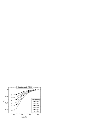
Figure 17: Fluctuation scaling for the random walker model with inhomogeneous impact, parameters $M=20000$, $W=100$, $s_{\mathrm{max}}=100$, $T=10000$ and various values of $\beta$. The case $\beta=0$ is the same curve as in the inset of Fig. 15. The $\alpha_{\mathrm{T}}(\Sigma_{W}\rightarrow 0)$ limit is well described by Eq. (18). For $\Sigma_{W}\gg\left\langle W\right\rangle$ every system displays a crossover to $\alpha_{\mathrm{T}}=1$.

IV.2 Critical fluctuations and finite size scaling

The mechanism how (spatial) correlations produce non-trivial values of $\alpha$ draws on some fundamental knowledge in statistical physics. Critical systems are known to exhibit anomalous fluctuations due to the presence of strong, but non-trivial correlations. These originate from the interactions of the internal constituents as for e.g. Ising spins.

It is instructive to consider the simple ferromagnetic case, like the nearest-neighbor Ising model reichl on a $d$ dimensional square lattice. Because this model does not a priori have dynamics, its analysis can be understood in the language of ensemble averages.

The number of spins is $N=L^{d}$, where $L$ is the linear size of the lattice. At the critical point local magnetization has a diverging correlation length, and the correlation function becomes of the power law form

$$C(\mathbf{r})\propto\frac{1}{r^{d-2+\eta}}.$$ (27)

The squared fluctuations of total magnetization [$\overline{\sigma}^{2}(M_{L})$] are known to be proportional to the susceptibility $\chi$, and for finite systems both quantities diverge at the critical point as

$$\overline{\sigma^{2}(M_{L})}\propto\chi\propto L^{d+\gamma/\nu}.$$ (28)

This is one of the well known results of finite size scaling (FSS) cardy .

The susceptibility can be calculated as the integral of the correlation function:

$$\chi=\frac{N}{k_{B}T}\int d^{d}\mathbf{r}C(\mathbf{r})\propto N\int^{L}\frac{d^{d}\mathbf{r}}{r^{d-2+\eta}}\propto L^{d+2-\eta}.$$ (29)

It is well known that the exponents in Eqs. (28) and (29) are related, $\gamma/\nu=2-\eta$ (Fisher’s law reichl ). At the critical point, due to the interactions between the spins, the susceptibility becomes super-extensive, i.e. it grows faster than $\propto L^{d}$, a typical sign of criticality.

Let us now consider an ensemble of finite Ising systems at the critical temperature with zero external field and with various linear sizes, and let the signal be the $N_{L,\uparrow}$ number of "up" spins. Of course the total number of up and down spins is constant:

$$N_{L,\uparrow}+N_{L,\downarrow}=L^{d},$$

and their difference gives the magnetization as

$$M_{L}=N_{L,\uparrow}-N_{L,\downarrow}.$$

With the notation $o(L^{p})/L^{p}\rightarrow 0$, at the critical point

$$\overline{N_{L,\uparrow}}=L^{d}/2+o(L^{d}).$$

On the other hand, the fluctuations of $M$ and $N_{\uparrow}$ are proportional, because

$$M_{L}=2N_{L,\uparrow}-L^{d},$$

and so

$$\overline{\sigma(N_{L,\uparrow})}^{2}=\overline{\sigma(M_{L})}^{2}/2\propto L^{d+2-\eta}+o(L^{d+2-\eta}).$$

Consequently, to a leading order, there exists EFS between the fluctuations and the mean of the number of up spins:

$$\overline{\sigma(N_{L,\uparrow})}^{2}\propto\overline{N_{L,\uparrow}}^{2\alpha_{\mathrm{E}}}$$

with

$$\alpha_{\mathrm{E}}=\frac{1}{2}+\frac{2-\eta}{2d}=\frac{1}{2}+\frac{\gamma/\nu}{2d}.$$ (30)

The above are true up to the upper critical dimension, which is $d_{c}=4$ for the Ising model cardy . The mean-field results can be recovered by substituting the corresponding values: $d=d_{c}=4$, $\gamma_{\mathrm{MF}}=1$, $\nu_{\mathrm{MF}}=1/2$, $\eta_{\mathrm{MF}}=0$. Finally $\alpha_{\mathrm{E,MF}}=3/4$, in agreement with the direct mathematical proof of Ellis and Newman ellis.cw . Moreover, at the critical point the susceptibility is superextensive, so $\chi$ must grow faster than $L^{d}$. This means that in Eq. (29) $d+2-\eta>d$, and thus $\eta<2$. On the other hand if $\eta$ is non-negative, then from the constraints $0\leq\eta<2$ and $d\geq 1$ it immediately follows that $1/2\leq\alpha_{\mathrm{E}}<1$. This range is also valid for the analogous behavior of all $n$-vector models.

This result is two-fold, depending on how we look at it:

1. The exponent $\alpha_{\mathrm{E}}$ resembles the finite-size scaling exponent of fluctuations/susceptibility. Thus in this case fluctuation scaling essentially finite-size scaling. The difference is that the FS calculation can be done even when there is no data available about "system size". Instead, because $N_{\uparrow}$ is a positive extensive quantity, we know that its expectation value will be proportional to the system size, and thus it can act as a surrogate variable for $L^{d}$. An anomalous value of the FS exponent can be related to critical behavior, although – as previous sections suggest – not necessarily. We will discuss this question in detail in Section IV.3.

2. The finding that when the constituents are long-range correlated gives rise to anomalous values of $\alpha$, leaves us with a recipe how to construct simple models that display $1/2<\alpha<1$. The simplest scenario is described in detail in Sections III.3.4 and IV.4.

What is the case with $N_{\uparrow}$ off the critical point? In the paramagnetic phase the mean number of up spins is exactly $N/2$, while the fluctuations are of order $N^{1/2}$, thus $\alpha_{\mathrm{E}}=1/2$. The ferromagnetic case is a more delicate issue, because the infinite system is not ergodic: spontaneous magnetization is symmetry breaking. For finite systems with a local (e.g. Glauber) dynamics it takes a finite (but very long) time for magnetization to change direction. The phenomenon is more easily interpreted via an (unrestricted) ensemble of equilibrium ferromagnets. Here still $\overline{f}=N/2$, because configurations magnetized up and down average out. The fluctuations on the other hand are macroscopic, $\overline{\sigma_{L}}\propto 2\overline{|M|}\propto L^{d}$. Thus $\alpha_{\mathrm{E}}=1$. In sum, the paramagnet-ferromagnet phase transition is signaled by FS as an abrupt change between the two universality classes (similarly to the Satake-Iwasa forest model satake.iwasa ; ballantyne.model ). At the critical point one finds intermediate exponents that can be calculated from the usual critical exponents. However, it is of fundamental importance that the anomalous FS is not observed in the order parameter $M$. Instead, it is observed in an extensive quantity, and only whose fluctuations reflect the anomalous fluctuations of the order parameter. FS is there in $M$, but with a trivial exponent: From finite size scaling $\overline{M}\propto L^{d-\beta/\nu}$. This, combined with Eq. (29) leads to $\overline{\sigma(M_{L})}\propto M^{(d+\gamma/\nu)/[2(d-\beta/\nu)]}$. Due to the hyperscaling relation $\gamma+2\beta=d\nu$ this means $\alpha_{E}=1$.

The critical point is a very special state of a system, while fluctuation scaling with $1/2<\alpha<1$ occurs very often. To make criticality a viable explanation for these non-trivial values of $\alpha$ it is important to notice that certain types of dynamics under strong external driving can self-organize to their critical state without the fine-tuning of any parameters bak.soc ; bak.book ; paczuski.solar . Many real life systems display the classical signs of self-organized criticality (such as power-law distributions, long-range correlations, etc.) and the value of $\alpha$ can help to understand the dynamical origins of these observations.

IV.3 Scaling and multiscaling

Scaling has a fundamental importance in statistical physics. It has found countless successful applications starting with critical phenomena stanley.phase , but more recently also outside the classical domain of physics, for example in ecology banavar.ecology . In many cases scaling is not bound to a specific set of system parameters like in the case of critical phenomena, but it is the generic behavior of the system as in polymers degennes.book , surface growth barabasi.stanley.book and self-organized criticality bak.soc . Mono-scaling or gap scaling means that the probability distribution of a quantity $f$ depends on the parameter $L$, usually the system size, as

$$\mathbb{P}(f,L)=f^{-1}F\left(\frac{f}{L^{\Phi}}\right),$$ (31)

where $F$ is a scaling function and $\Phi$ is some constant. This form can account for a number of observations about power law behavior in real systems.

Both gap scaling and fluctuation scaling characterize a large number of complex systems. Nevertheless, for the same quantity only one can be true except in a special case: If a quantity shows both gap scaling and fluctuation scaling, then this automatically implies $\alpha=1$. One can reverse this argument: If for a quantity one finds fluctuation scaling with $\alpha<1$ then it cannot exhibit gap scaling.

The proof is straightforward. Any moment of $f$ can be calculated as

$$\overline{f^{q}_{L}}=\int_{f_{0}}^{\infty}dff^{q}\mathbb{P}(f,L)\simeq K_{q}L^{q\Phi},$$ (32)

where "$\simeq$" denotes asymptotic equality and $K_{q}>0$. From Eq. (32) it follows that

$$\overline{\sigma^{2}_{L}}=\overline{f^{2}_{L}}-\overline{f_{L}}^{2}\simeq$$

$$K_{2}L^{2\Phi}-K_{1}^{2}L^{2\Phi}=(K_{2}-K_{1}^{2})L^{2\Phi}.$$ (33)

We combine EFS and Eq. (33), eliminate $L$ and find that now $\overline{\sigma^{2}_{L}}\propto\overline{f_{L}}^{2}$, i.e., $\alpha=1$.

The only possibility for the coexistence of gap scaling (31) and fluctuation scaling (5) with $\alpha<1$ is when the constant factor in the variance vanishes:

$$(K_{2}-K_{1}^{2})=0.$$

In this case the gap scaling form does not describe the variance, that is instead given by the next order (correction) terms. Nevertheless, even if it is so, the leading order of the variance is still zero, and consequently $F$ is proportional to a Dirac-delta:

$$F\left(\frac{f}{L^{\Phi}}\right)\propto\delta\left(f/L^{\Phi}-K_{1}\right).$$

This case is pathological, and it is usually not considered as scaling. In fact, the previous section contained one such example: The number of up spins in a critical Ising model follows this sort of statistics. Fluctuations scale anomalously ($\overline{\sigma^{2}_{L}}\propto L^{d+2-\eta}$), whereas their leading order vanishes because $\overline{f^{2}}\simeq\overline{f}^{2}\simeq L^{2d}/4$. Such strange scaling arises as a sign of criticality when the scaling variable is an extensive quantity, for which only the fluctuations are connected to those of the order parameter.

For example, in ecology there do exist species with $\alpha\approx 1$, for which a gap scaling form of the probability density of $f$ could be valid. However, this value is by no means universal (cf. Fig. 1). Similarly, $\alpha<1$ was observed for Internet router traffic barabasi.fluct or the traded value on stock markets eisler.non-universality . These quantities cannot have a gap scaling form.

Instead of gap scaling, one can assume multiscaling, but the results do not change crucially. A probability distribution shows multiscaling if its size dependence is of the form

$$\ln\mathbb{P}(f,L)/\ln(L/L_{0})=-F[\ln(f/f_{0})/\ln(L/L_{0})],$$ (34)

where $f_{0}$ and $L_{0}$ are appropriately chosen constants. The moments can be calculated by expressing the density function from Eq. (34) and substituting into the definition

$$\overline{f_{L}^{q}}=\int_{0}^{\infty}f^{q}\mathbb{P}(f,L)df=$$

$$\int_{0}^{\infty}f^{q}\left(\frac{L}{L_{0}}\right)^{-F[\ln(f/f_{0})/\ln(L/L_{0})]}df\simeq$$

$$f_{0}^{q}\left(\frac{L}{L_{0}}\right)^{qa(q)}\left(\frac{L}{L_{0}}\right)^{-F[a(q)]}\simeq K_{q}L^{\tau(q)}.$$

The usual approach is that the value of the integral is dominated by the point $f_{*}(q)$ where the integrand is maximal. Then

$$a(q)=\frac{\ln[f_{*}(q)/f_{0}]}{\ln(L/L_{0})},$$

and

$$\tau(q)=\max_{a}[qa-F(a)],$$

or equivalently $\frac{\tau(q)}{\partial q}=a.$ Now we are back at the same situation as with gap scaling, since

$$\overline{f_{L}}\simeq K_{1}L^{\tau(1)}$$

and

$$\overline{\sigma_{L}^{2}}=\overline{f_{L}^{2}}-\overline{f_{L}}^{2}\simeq K_{2}L^{\tau(2)}-K_{1}^{2}L^{2\tau(1)}.$$

One expects that $\tau(2)\geq 2\tau(1)$, because the variance must remain non-negative for arbitrarily large $L$. If $\tau(2)>2\tau(1)$ then the first term dominates $\overline{\sigma_{L}^{2}}$, and $\alpha=\frac{\tau(2)}{2\tau(1)},$ but this value is greater than $1$. For example Tebaldi et al. stella.btw report that in the Bak-Tang-Wiesenfeld sandpile model of $L$ linear size, the distribution of the number of topplings $f$ in an avalanche follows $\overline{f^{q}_{L}}\propto L^{\tau(q)}$ with $\tau(1)\approx 2$, and $\tau(2)\approx 4.7$. This results in an $\alpha\approx 1.17$.

The other possibility is again $\tau(2)=2\tau(1)$, and $\alpha=1$ (unless the leading order terms in $\sigma^{2}$ compensate to zero). This solution offers nothing new compared to gap scaling. Such relationships can be seen, e.g., in the very same BTW model for the distribution of the area affected by avalanches stella.btw .

The conclusion: If a quantity shows gap scaling with a scaling function which is not fully degenerate (not a Dirac-delta), it must follow $\alpha=1$. If there is multiscaling, then fluctuation scaling with $\alpha>1$ is also possible, but such values are rarely observed and should be taken with care.

IV.4 Binary forest model

In this section we introduce a toy model that can be used to better illustrate the ideas of Sections IV.2-IV.3. Moreover, we will show that those are in full analogy with the findings of Section II.3.2 for the reproductive activity of trees. For an easier understanding we will present the model in that language.

Let us consider a forest that consists of $N$ trees. For simplicity we also assume that these are situated on a one-dimensional regular lattice, but any higher dimensional generalization is straightforward. In the year $t$ the reproductive activity (i.e. seed count) of every tree $n$ is characterized by a random variable $V_{n}(t)$. Again, for simplicity we consider $V$’s as binary variables, which are $1$ with probability $p$ and $0$ with probability $1-p$. Because it takes several years for a new tree to reach its full reproductive capabilities, given that the observation period is short enough, we can neglect the changes in $N$ due to seed production and tree growth.

The year-to-year correlations in seed counts are neglected. On the other hand, it is known koenig.masting that the reproductive activity of forests exhibits long-range spatial dependence, with significant positive correlations for distances of thousands of kilometers. The distance dependence can be fitted approximately by

$$C(\Delta n)\propto\left\langle V_{n}V_{n+\Delta n}\right\rangle-\left\langle V_{n}\right\rangle^{2}\propto\Delta n^{2H_{V}-2},$$ (19)

see Section II.3.2. The total seed count is given by the usual form

$$f_{N}=\sum_{n=1}^{N}V_{n}.$$

The standard deviation of the sum of random variables correlated according to Eq. (19) scales as

$$\sigma_{N}=\sqrt{\left\langle f_{N}^{2}\right\rangle-\left\langle f_{N}\right\rangle^{2}}\propto N^{H_{V}}$$

with $H_{V}$ being the Hurst exponent [cf. Eq. (10)], whereas

$$\left\langle f_{N}\right\rangle=pN.$$

The two equations can be combined into TFS with

$$\alpha_{\mathrm{T}}=H_{V}.$$ (20)

To the careful reader it should be clear that almost the same model was discussed in Section IV.2. There we argued that in a critical Ising model whether any given spin points upwards ($1$) or downwards ($0$) is essentially a binary random variable with $p=1/2$. Moreover the spin alignments are power-law correlated in space, such that the power of the decay is related to the FS exponent $\alpha$. This was expressed by Eq. (30), which is essentially equivalent to (20). The binary forest model only differs from the Ising case in that correlations between the random variables are given a priori, and not generated by the thermodynamics.

Now we can move on to simulation results. Fig. 18 shows the dependence of $\sigma_{N}$ on $N$ and $\left\langle f\right\rangle$, the two plots are basically equivalent due to $\left\langle f\right\rangle=pN$. Fig. 19(left) illustrates that the fluctuations in systems of the same size increase rapidly with $H_{V}$. This is due to a strong synchronization of the individual constituents [see Fig. 19(right)]. The relationship (20) is illustrated in Fig. 20.

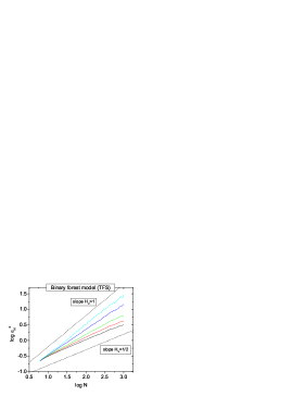
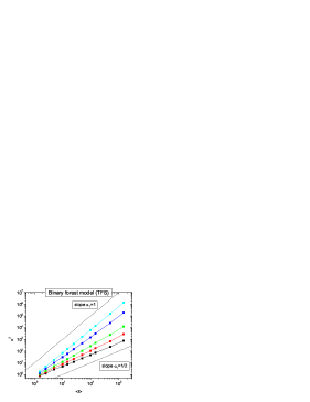
Figure 18: (left) Scaling plots of $\sigma$ versus $N$ generated by Detrended Fluctuation Analysis of $V_{n}(t)$ in the binary forest model. The slopes correspond to the (spatial) Hurst exponents $H_{V}\approx 0.5,\dots,0.95$ from bottom to top, see Eq. (10). (right) Scaling plots $\sigma$ versus $\left\langle f\right\rangle$ for FS in the same data. The slopes correspond to the values of $\alpha_{\mathrm{T}}\approx 0.5,\dots,0.95$.

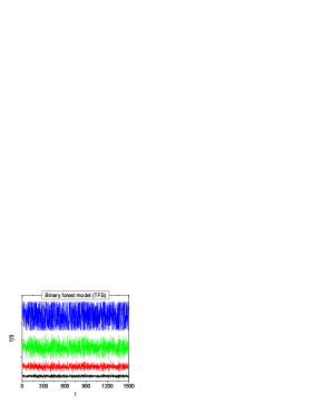
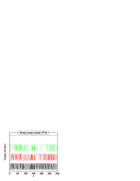
Figure 19: (left) Examples of $f_{i}(t)$ time series for a "forest" with $N=300$ "trees". The Hurst exponent $H_{V}$ between the trees was varied: $H_{V}\approx 0.5,0.65,0.8,0.95$ increasing from bottom to top. The data were shifted by the addition of a constant, but they were not stretched in any way. One can see that due to the increasing synchronization of the constituents, relative fluctuations increase rapidly. (right) Snapshot of $V_{i,n}$ series (at a fixed time $t$) for a forest with $N=300$ elements. The data were shifted by the addition of a constant. The Hurst exponent $H_{V}$ between the elements was varied: $H_{V}\approx 0.5,0.65,0.8,0.95$ increasing from bottom to top. Spatial synchronization increases with the growth of the Hurst exponent.

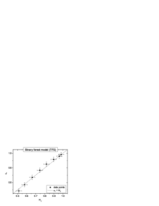
Figure 20: The equality $\alpha_{\mathrm{E}}=H_{V}$ (dotted line) in simulations of the binary forest model. The measurement points align very closely to the line, with some statistical deviations.

V Discussion

In this section we present our view about unsettled questions related to fluctuation scaling. We also discuss recent, sometimes controversial techniques that might help the understanding of FS.

V.1 Separation of global and local dynamics

In Section III.2 we argued that a system whose internal dynamics can be mapped onto the central limit theorem displays fluctuation scaling with $\alpha=1/2$. On the other hand, if one imposes a strong external driving to the system, the behavior crosses over to $\alpha=1$. One example was shown in Section IV.1 in the case of random walks on complex networks. There the fluctuation was given by Eq. (26), which has the structure

$$\sigma^{2}_{i}=\left\langle f_{i}\right\rangle+A^{2}\left\langle f_{i}\right\rangle^{2},$$ (35)

where $A$ is proportional to the strength of the external driving. If $A\ll 1$ one finds $\alpha=1/2$, whereas in the strongly driven limit $A\gg 1$ the first term is negligible and $\alpha=1$.

Now assume that we do not know the strength of external driving and we want to approximate it from data. We can introduce the global activity $F(t)$ of the system as a sum over all constituents:

$$F(t)=\sum_{i=1}^{N}f_{i}(t).$$ (36)

Ref. barabasi.separating suggests that if our system has many elements, then $F(t)$ will be proportional to the external force, because the independent fluctuations of the elements average out in the sum (36), and what remains is only the factor of the common external driving. This argument implicitly assumes, that the external force contributes to the fluctuations of the elements in a coherent way, i.e., $f_{i}(t)$ can be written in the form

$$f_{i}(t)=f_{i}^{\mathrm{int}}(t)+f_{i}^{\mathrm{ext}}(t),$$ (37)

where

$$f_{i}^{\mathrm{ext}}(t)=A_{i}F(t).$$ (38)

This formula is a form of linear response, where: (i) $A_{i}$ is not allowed to depend on time because of stationarity. (ii) More importantly, all nodes are affected by driving instantaneously or with the same constant time lag.

After the summation of Eq. (36) we find that it is consistent with Eq. (37), if the normalization condition $\sum_{i}A_{i}=1$ is satisfied. In order to keep Eqs. (35) and (37) consistent in the strongly driven limit, the only possible choice is

$$A_{i}=\frac{\left\langle f_{i}\right\rangle}{\left\langle F\right\rangle}.$$ (39)

By this definition automatically $\left\langle f_{i}^{\mathrm{int}}\right\rangle=0$ and $\left\langle f_{i}^{\mathrm{ext}}\right\rangle=\left\langle f_{i}\right\rangle$. All time series have finite standard deviations, which are defined in the usual way, for example $\sigma_{F}=\sqrt{\left\langle F^{2}\right\rangle-\left\langle F^{2}\right\rangle}$. With these

$$\sigma_{i}^{\mathrm{ext}}=\frac{\sigma_{F}}{\left\langle F\right\rangle}\left\langle f_{i}\right\rangle,$$ (40)

so the external component follows FS with $\alpha=1$ in any system. This appears consistent with the fact that in strongly driven systems $f$ itself also shows $\alpha=1$, not only the external component. However, this is in fact just a trivial consequence of how the external component was defined.

Ref. barabasi.separating calls the process of assigning the internal and external components "noise separation", and claims that the procedure works well for the random walk model. For each node they define a noise ratio

$$\eta_{i}=\frac{\sigma_{i}^{\mathrm{ext}}}{\sigma_{i}^{\mathrm{int}}},$$

which is zero in the absence of external driving, and large when the fluctuations of the external component are dominant.

It would be tempting to attribute the real world observations of $\alpha\approx 1$ to external driving, and show that in these cases typically $\eta\gg 1$. However, we will demonstrate on some examples that noise separation has strong limitations.

Ref. barabasi.separating finds that the fluctuations of Internet (Abiline backbone) traffic show TFS with $\alpha=1/2$ and typically $\eta\sim 0.1$. While this appears very convincing, a more detailed analysis of a subset of the same data duch.internet instead finds $\alpha=0.7-0.8$. The latter study suggests congestion as the origin of the increase value of $\alpha$, and does not assume any external driving force.

Ref. barabasi.fluct reports, that river level fluctuations fall into the class $\alpha=1$. It seems plausible that water levels fluctuate due to rainfall on the river basin, which can be understood as external driving. However, noise separation is impossible here, because the driving is not coherent. The global factor $F(t)=\sum_{i}f_{i}(t)$ is meaningless, because the response times of the water level, and the timing of precipitation vary from river to river. Hence Eq. (38) is not valid.

To our knowledge, our study eisler.non-universality was the first to reveal fluctuation scaling in the trading activity of stocks. Noise separation was carried out there, finding that the typical value of $\eta_{i}$ increases with the time window $\Delta t$. Because $\alpha$ also shows a similar tendency (cf. Fig. 6), we suggested that external driving must play a role in this effect. We also argued that this is because information needs a finite time to spread on the market. On the scale of a few minutes the role of external information is small and localized, whereas on the long run trading is dominated by the external macroeconomic trends and news.

Later we proposed a much simpler explanation eisler.unified , which was also summarized in Sections II.3.4 and III.3.1 of this review. In the stock market (and human dynamics, see Section II.4.2) one observes, that for long times $\alpha(\Delta t)=\alpha^{*}+\gamma\log\Delta t$ and $H_{i}=H^{*}+\gamma\log\left\langle f_{i}\right\rangle$ with some $\gamma>0$. These laws have not yet been related to any external force, even though the possibility cannot be ruled out.

How would noise separation work in this case?

1. Clearly $\sigma_{F}\propto\Delta t^{H_{F}}$, with $H_{F}\approx\max_{i}H_{i}$, because $F$ is the sum of all $f_{i}$’s, and the scaling of the sum is dominated by the highest Hurst exponent.

2. $\sigma_{i}^{\mathrm{ext}}\propto\sigma_{F}\propto\Delta t^{H_{F}}$. On the other hand, if $\sigma_{i}^{\mathrm{ext}}<\sigma_{i}^{\mathrm{int}}$, then one expects that qualitatively $\sigma_{i}^{\mathrm{int}}\propto\Delta t^{H_{i}}$.

3. Thus the ratio $\eta_{i}=\sigma_{i}^{\mathrm{ext}}/\sigma_{i}^{\mathrm{int}}$ should typically grow as long as $\eta_{i}<1$. This observation of Ref. eisler.non-universality is hence no proof of any particular external influence.

While to present further calculations is not the purpose of this review, we believe, that $\eta\simeq 1$ can arise from spurious effects. A value $\eta_{i}>1$ consistently, for many nodes has only been observed in a single study where $\eta\simeq 1.5$ jiang.fluxes . Our present understanding is that noise separation has a limited range of applicability.

Finally, we would like to point out that to identify the ensemble average (36) with some external force is somewhat controversial. Since we do not have any information about the origin or the physical meaning of the factor $F(t)$, it is probably more appropriate to call this and $f_{i}^{\mathrm{ext}}$’s global and not external factors. Accordingly, $f_{i}^{\mathrm{int}}$’s are better called local, rather than internal factors when it is unknown how much they represent internal processes at the nodes.

V.2 Limit theorems for sums of random variables

In Section III.2.1 we briefly remarked on the connection of $\alpha=1/2$ to the central limit theorem. We recall that $f$ is written as a sum over the constituents (other random variables) whose number $N$ we will consider as time independent:

$$f=\sum_{n=1}^{N}V_{n}.$$

Let us assume that a general form of central limit theorem is applicable, so that

$$\frac{\sum_{n=1}^{N}V_{n}-N\left\langle V\right\rangle}{N^{\alpha}\Sigma_{V}}\rightarrow X,$$ (41)

where $X$ is some random variable and "$\rightarrow$" means convergence in distribution for $N\rightarrow\infty$. In the language of FS the same equation reads

$$\frac{\sum_{n=1}^{N}V_{n}-\left\langle f\right\rangle}{K\left\langle f\right\rangle^{\alpha}}\rightarrow X,$$ (42)

where $K$ is a constant. The conceptual difference is only that since we know that $\left\langle f\right\rangle=N\left\langle V\right\rangle$, we can use $\left\langle f\right\rangle\left\langle V\right\rangle^{-1}$ as a surrogate variable for $N$.

This analogy tells us that the appearance of FS throughout disciplines might be due to the generality of certain limit theorems. The trivial example is of course that of i.i.d. variables with positive mean and finite variance, leading to the value $\alpha=1/2$, but there are several other cases.

If the $V$’s are i.i.d., but their distribution decays asymptotically as $\mathbb{P}(f)\propto f^{-(\lambda+1)}$ with $0<\lambda<2$, then the Lévy-Gnedenko central limit theorem is applicable feller . That is in spirit similar to Eq. (41), with $\alpha=1/\lambda$. The difference is that $\sigma$, and if $\lambda\leq 1$ even $\left\langle f\right\rangle$ is infinite. However, for $N<\infty$ they will have some finite effective value, which can show apparent fluctuation scaling with some non-trivial value of $\alpha$.

Contrary to the relative simplicity of independent (and possibly identically distributed) random variables, dependent variables can be extremely diverse. They have no general theory, and the number of universality classes/limit theorems is infinite. Their structure is not always fully described by pairwise correlations and Hurst exponents (cf. Sections IV.2-IV.4). In these cases sometimes there exists no limit distribution, or, e.g., $\alpha<1/2$ or $\alpha>1$ in Eq. (41) clt1 .

Even for the usual $1/2\leq\alpha\leq 1$ values there is only a limited set of results, here we only mention a few inspired by statistical mechanics. In a series of papers Ellis, Newman and Rosen ellis.newman ; ellis.cw ; ellis.rosen show that in some statistical mechanical systems physical quantities can obey Eq. (41) with $\alpha=1-1/2k$, where $k$ is a non-negative integer. For example, in the Curie-Weiss mean-field model the number of up spins obeys $k=2$ and $\alpha=3/4$ at criticality, and the distribution of $X$ can also be given explicitly. In Section IV.2 we arrived at the same exponent using heuristic arguments. Baldovin and Stella baldovin.clt recently published some more general results on a mean-field theory of strongly correlated random variables. In their model fine-tuning the strength of correlations allows for any $1/2\leq\alpha\leq 1$, much in the spirit of Section IV.4 and Ref. ballantyne.correls .

V.3 The connection of ensemble and temporal averages

Let us now return to the connection between the TFS

$$\sigma_{i}(\Delta t)\propto\left\langle f_{i}\right\rangle^{\alpha_{T}},$$ (3)

and the EFS

$$\overline{\sigma_{N}}(\Delta t)\propto{\overline{f_{N}}}^{\alpha_{E}}$$ (5)

laws. These correspond to two definitions of the statistical quantities: (i) for Eq. (3) the mean and the standard deviation are calculated as temporal averages; (ii) for Eq. (5) they are calculated on an ensemble of subsystems of the same size.

For the mere existence of such quantities it is necessary to assume that: (i) signals with the same mean have the same statistical properties, and the processes are stationary; or (ii) systems of the same size can be considered elements of the same statistical ensemble, which is a kind of a homogeneity condition. In real systems neither of these conditions holds exactly, but they often prove to be good approximations. A deviation from these assumptions is one possible source of the observed broadening of the scaling plots. For example, in the case of precipitation data in Section II.4.3 we found that mean precipitation is not the only determinant of the amplitude of fluctuations. Areas with the same mean precipitation are not equivalent, because they can correspond to very different climates. Factors such as height and geographical position are also relevant.

A related concern is the presence of correlations gaston.mcardle . The observations may be correlated in space or time. (i) Two nodes (e.g., populations or weather stations) which are located close to each other can have significant cross-correlations. Fits can be biased, because the observations are not independent. (ii) The signals of individual nodes can have strong temporal autocorrelations, which can amplify statistical errors when the time series are not long enough smallsampletaylor .

A more delicate question is the connection between the two types of FS, which has been very vaguely investigated in real systems so far. First of all, the two factors cannot be separated completely. McArdle et al. mcardle.variation point out this problem through the example of animal populations. (i) The measurement of the number of individuals in an area takes a finite time. There is an in and outflow of individuals, so the number fluctuates. Thus temporal dynamics can affect the results. (ii) If we want to measure the time series of the size of a given population, we have to assign a spatial scale as what to consider a population. The temporal dynamics will depend on this spatial scale of sampling, possibly in a non-trivial way.

Taylor and Woiwod taylor.woiwod conducted a very large scale study of the two (temporal and ensemble) FS laws in animal populations. A systematic comparison is possible when the same sites sampled are at the same time mcardle.variation . Taylor and Woiwod calculated the temporal and spatial means and standard deviations of the abundance of some aphids, moths and bird, then calculated $\alpha_{\mathrm{T}}$ and $\alpha_{\mathrm{E}}$ for each species.

First of all, they found that the temporal and ensemble means of population differ significantly. Thus it is not surprising that the values of $\alpha$ differ as well. There was absolutely no systematic relationship between $\alpha_{\mathrm{T}}$ and $\alpha_{\mathrm{E}}$, and even the same species can show several such values depending on its natural environment. Rather interestingly, the only systematic dependence between species is the presence of positive correlations between the value of $\alpha$’s, and average population size. For example, for temporal data this means that across species $\alpha_{\mathrm{T}}$ is correlated with $1/M\sum_{i=1}^{M}\left\langle f_{i}\right\rangle$. The correlations are present in both cases, although stronger for the temporal variant. Taylor and Woiwod taylor.woiwod also suggested, that the interactions between individuals might contribute to the ensemble law more than to the temporal one.

In some studies such as ecology or climatology the definition of the spatial scale comes naturally. Still, most systems have some hierarchical structure on which a degree of aggregation is possible. For example, it is possible to analyze the fluctuations of Internet traffic at the autonomous system level instead of the router level, which might have a different dynamics. On the stock market TFS holds not only for individual stocks, but also when we consider the trading activity of industry sectors uponrequest .

In sum, the relationship between ensemble and temporal fluctuation scaling is rather unclear in real systems. The exponents $\alpha_{\mathrm{E}}$ and $\alpha_{\mathrm{T}}$ are seldom calculated for the same system, and when they are calculated, they have different values.

V.4 Fluctuation scaling for growth rates

To be able to interpret FS for temporal fluctuations one has to assume that the underlying system is stationary. For example, in the binary forest model of Section IV.4 we assumed that the number of trees is constant and we neglect the contribution of reproduction to the population. To depart from stationarity, we can consider a growing population of $N_{i}(t)$ individuals, all of which can reproduce at a time $t$ [$V_{i,n}(t)=$ the number of offsprings], die [$V_{i,n}(t)=-1$] or do nothing [$V_{i,n}(t)=0$]. The population can now be written as a sum

$$N_{i}(t+1)=N_{i}(t)+\sum_{n=1}^{N_{i}(t)}V_{i,n}(t).$$

$N_{i}(t)$ is obviously not stationary, because its distribution depends on its value in the previous time step. Nevertheless, one can still construct something similar to TFS by using a restricted ensemble average as follows.

Let us define the growth rate of a population as

$$f_{i}(t)=N_{i}(t+1)-N_{i}(t).$$

Now let us make an ensemble of growth observations when the initial population was $N$. The growth rate in this restricted sample is given by

$$f_{N}=\sum_{n=1}^{N}V_{n}.$$

Because $f$ can be negative, to postulate TFS for size dependence it is more convenient to use $N$ and not $\left\langle f\right\rangle$ as the scaling variable. We conjecture

$$\sigma_{N}=\sqrt{\left\langle f_{N}^{2}\right\rangle-\left\langle f_{N}\right\rangle^{2}}\propto N^{\alpha}$$ (43)

in the spirit of the previous sections, and this is exactly what is found in many systems.

Keitt and Stanley show keitt.pop ; keitt.scaling that the growth rate fluctuations of animal populations scale as a non-trivial power of the initial population $N$. The finding is not specific for population growth, but occurs in many settings where a positive quantity fluctuates by the addition and subtraction of increments. The same behavior was found by Lee et al. stanley.firm for the growth rates of business firms, and Amaral et al. amaral.growth even presents a model of the complex structure of the business growth process which predicts the correct exponent.

Jánosi and Gallas janosi.danube criticize these results, and show the same distribution of growth rates and the scaling law (43) for the water level fluctuations of the river Danube, which trivially must have a structure that is very different from business firms. Moreover, they show that the daily absolute change of water level scales with the average water level on the same day, and there is a clear crossover behavior between two scaling regimes with $\alpha=1/2$ and $\alpha=1$. A related study by Dahlstedt and Jensen dahlstedt.river estimates $\alpha\approx 0.9-1$, and suggests that FS can be decomposed into two distinct scaling laws: $\sigma_{A}\propto A^{a}$ and $\left\langle f_{A}\right\rangle\propto A^{b}$, where $A$ is the area of the river basin.

From the above it is clear that the size-dependent scaling of growth rate fluctuations is a variant of fluctuation scaling for nonstationary (growing) populations. The same formalism can be applied in both cases, and many results could be mutually applied.

VI Conclusions

The aim of this review was to provide a broader perspective on Taylor’s law and fluctuation scaling, and to encourage the collaboration between disciplines where these phenomenona are observed. We also outlined a classification scheme on the meaning of the FS exponents. The main conclusion is that several types of mechanisms can lead to the same value of $\alpha$. A similar concern was formulated in the 1982 paper of Taylor and Woiwod taylor.woiwod :

"Extrapolation of dynamic principles from […] observation is likely to be misleading. We find great differences between [species], but the overlap is also very large. Whilst it is improbable that the details of […] behaviour in a bird and an aphid would be alike, there are common elements in the […] structure of their populations."

While fluctuation scaling alone is not enough to identify the underlying dynamics of a system, it is useful for excluding some possibilities, and for rejecting certain models which would generate unrealistic $\alpha$’s. Empirical data from virtually all fields of science display fluctuation scaling, and so it is possible to make statements about almost any system where such data is available. For this very reason, in order to deepen our understanding of the phenomenon, it is becoming increasingly important to bridge the gap between several disciplines. But the most puzzling question still remains: Why do, for example, email traffic, stock market trading and the printing activity in a computer lab behave in similar, non-trivial ways? Some insights can be gained from the time window dependence of $\alpha$. That can reveal whether on some time scale the behavior of the system reduces to something simpler or possibly trivial. One can also make efforts to decompose the signals into well-defined constituents, so that a mean-field model based on sums of random variables can be applied. We believe that a possible common origin of all fluctuation scaling laws is the generality of these underlying mean-field type mathematical structures.

Appendix A The components of the fluctuation $\sigma^{2}$

A large part of this review is concerned with the standard deviation of the sums of random variables. This is defined as

$$\sigma^{2}=\left\langle\left(\sum_{n=1}^{N}V_{n}\right)^{2}\right\rangle-\left\langle\sum_{n=1}^{N}V_{n}\right\rangle^{2},$$

where $V_{n}$ are the individual (not necessarily independent) random variables, and $N$ is the number of these variables which itself can be random.

Let $\mathbb{P}(N)$ be the probability that the number of variables is $N$. The sum of $N$ variables can be written as $V_{N}=\sum_{n=1}^{N}V_{n}$. Let $\mathbb{P}(V_{N})$ denote the density function of this sum when $N$ is fixed. Then the standard deviation of the sum when $N$ itself is a random variable is

$$\sigma^{2}=\sum_{N}\mathbb{P}(N)\int dV_{N}\mathbb{P}(V_{N})V_{N}^{2}-$$

$$\left(\sum_{N}\mathbb{P}(N)\int dV_{N}\mathbb{P}(V_{N})V_{N}\right)^{2}=$$

$$\sum_{N}\mathbb{P}(N)\underbrace{\left[\underbrace{\int dV_{N}\mathbb{P}(V_{N})V_{N}^{2}}_{\left\langle V^{2}_{N}\right\rangle}-\underbrace{{\left(\int dV_{N}\mathbb{P}(V_{N})V_{N}\right)^{2}}}_{\left\langle V_{N}\right\rangle^{2}}\right]}_{\Sigma^{2}_{V_{N}}=N\Sigma^{2}_{V}}+$$

$$\sum_{N}\mathbb{P}(N)\underbrace{{\left(\int dV_{N}\mathbb{P}(V_{N})V_{N}\right)^{2}}}_{\left\langle V_{N}\right\rangle^{2}=N^{2}\left\langle V\right\rangle^{2}}-$$

$$\left(\sum_{N}\mathbb{P}(N)\underbrace{\int dV_{N}\mathbb{P}(V_{N})V_{N}}_{\left\langle V_{N}\right\rangle=N\left\langle V\right\rangle}\right)^{2}=\Sigma^{2}_{V}\underbrace{\sum_{N}\mathbb{P}(N)N}_{\left\langle N\right\rangle}+$$

$$\left\langle V\right\rangle^{2}\underbrace{\left[\underbrace{\sum_{N}\mathbb{P}(N)N^{2}}_{\left\langle N^{2}\right\rangle}-\underbrace{\left(\sum_{N}\mathbb{P}(N)N\right)^{2}}_{\left\langle N\right\rangle^{2}}\right]}_{\Sigma^{2}_{N}}$$

Thus finally

$$\sigma^{2}=\Sigma^{2}_{V}\left\langle N\right\rangle+\left\langle V\right\rangle^{2}\Sigma^{2}_{N}.$$

In the case when the $V_{n}$’s are strongly (i.e., power law) correlated $\Sigma^{2}_{V_{N}}=\Sigma^{2}_{V}N^{2H_{V}}$ where $H_{V}$ is the Hurst exponent as defined in Eq. (10), and so

$$\sigma^{2}=\Sigma^{2}_{V}\left\langle N^{2H_{V}}\right\rangle+\left\langle V\right\rangle^{2}\Sigma^{2}_{N}.$$

The correlations in $N$ are not reflected directly in this expression. Instead, they affect how $\Sigma_{N}$ changes with the time window size $\Delta t$ as pointed out in Section III.3.1.

Appendix B Tweedie models and impact inhomogeneity

In this appendix we prove that origin of the non-trivial $\alpha$ values in the formalism of Kendal kendal.ecological ; kendal.blood is essentially due to impact inhomogeneity. Kendal’s formalism is based on the so-called Tweedie exponential dispersion models penis . These form a family of random distributions, characterized by the logarithmic cumulant function (see Ref. penis , p. 1516)

$$K_{f}^{*}(s)=\ln\left\langle e^{sf}\right\rangle_{f}=\lambda_{\theta}[g_{\theta}(s)-1],$$ (44)

where $s$ is a constant and $f$ is the random variable. We use natural logarithms ($\ln$), as opposed to other parts of this review, where we used $10$-base logarithms ($\log$). We also introduced the notation $\left\langle x\right\rangle_{y}=\int_{0}^{\infty}dye^{xy}$. The two terms above are

$$\lambda=\frac{a-1}{ka}\left(\frac{k\theta}{1-a}\right)^{a},$$ (45)

and

$$g_{\theta}(s)=\left(1+\frac{s}{\theta}\right)^{a}.$$ (46)

$\theta>0$ and $a<0$

As pointed out both by Kendal kendal.ecological and Bar-Lev and Enis penis , the form (44) is characteristic of compound Poisson processes feller . These are distributions of random variables of the following type:

$$f=\sum_{n=1}^{N}V_{n},$$

where $N$ is Poisson distributed, and $V_{n}$ are i.i.d. random variables. The proof is straightforward, however, we include it here for completeness. The density function of a compound Poisson variable $f$ can be written as a complete probability

$$P(f)=\sum_{N=0}^{\infty}P(f|N)P(N).$$

The characteristic function is given by

$$\left\langle e^{sf}\right\rangle_{f}=\int dfe^{sf}P(f)=$$

$$\sum_{N=0}^{\infty}P(N)\int dfe^{sf}P(f|N)=$$

$$\sum_{N=0}^{\infty}P(N)\int dfe^{sf}P(V_{1}+V_{2}+\dots V_{N})=$$

$$\sum_{N=0}^{\infty}P(N)\left\langle e^{sV}\right\rangle_{V}^{N}.$$

For the last equality we used the property of the characteristic function that $\left\langle e^{s\sum_{n}V_{N}}\right\rangle=\left\langle e^{sV}\right\rangle^{N}.$ Then, knowing that if $N$ is Poisson distributed with mean $\left\langle N\right\rangle$ then its characteristic function is $\left\langle e^{tN}\right\rangle=e^{\left\langle N\right\rangle(e^{t}-1)}$,

$$\sum_{N=0}^{\infty}P(N)\left\langle e^{sV}\right\rangle_{V}^{N}=\left\langle e^{N\ln\left\langle\exp(sV)\right\rangle_{V}}\right\rangle_{N}=$$

$$e^{\left\langle N\right\rangle(\left\langle\exp(sV)\right\rangle_{V}-1)}=\left\langle e^{sf}\right\rangle_{f}.$$ (47)

The next step is to compare Eqs. (45), (46) and (47). One finds that for the Tweedie model

$$\left\langle e^{sV}\right\rangle_{V}=g_{\theta}(s)=\left(1+\frac{s}{\theta}\right)^{a}.$$

This is the characteristic function of a gamma distribution. Its moments can be determined as usual:

$$\left\langle V\right\rangle=\left[\frac{\partial}{\partial s}\left\langle e^{sV}\right\rangle_{V}\right]_{s=0}=a\theta^{-1},$$

$$\left\langle V^{2}\right\rangle=\left[\frac{\partial^{2}}{\partial s^{2}}\left\langle e^{sV}\right\rangle_{V}\right]_{s=0}=a(a-1)\theta^{-2},$$

$$\Sigma^{2}_{V}=\left\langle V^{2}\right\rangle-\left\langle V\right\rangle^{2}=-a\theta^{-2}.$$

For the expectation value of the Poisson variable:

$$\left\langle N\right\rangle=\lambda=\frac{a-1}{ka}\left(\frac{k\theta}{a-1}\right)^{a}\propto\theta^{a}.$$

Furthermore,

$$\left\langle f\right\rangle=\left[\frac{\partial}{\partial s}K_{f}^{*}(s)\right]_{s=0}=\lambda a\theta^{-1},$$

and

$$\sigma^{2}=\left[\frac{\partial^{2}}{\partial s^{2}}K_{f}^{*}(s)\right]_{s=0}=\lambda a(a-1)\theta^{-2}.$$

Let us recall, that also $\lambda$ contains terms with $\theta$. Simple calculation yields

$$\sigma^{2}=k\left\langle f\right\rangle^{2\alpha},$$

where $2\alpha=(a-2)/(a-1)$. Consequently:

1. Let us introduce $\beta=-1/a$. Then

   $$\left\langle V\right\rangle\propto\left\langle N\right\rangle^{\beta},$$ (17)

   which is impact inhomogeneity.

2. Moreover, $\sigma\propto\left\langle f\right\rangle^{\alpha}$ with

   $$\alpha=\frac{1}{2}\left(1+\frac{\beta}{\beta+1}\right),$$ (18)

   exactly the same relationship as in Section III.3.2.

Appendix C Fluctuations in the network random walker model

This section contains calculations starting from the master equation (21). The total number of visitations to node $i$ is the sum over all steps. The substitution of Eq. (21) gives

$$f_{i}=\sum_{s=1}^{s_{\mathrm{max}}}N_{i}(s)=\sum_{s=0}^{s_{\mathrm{max}}-1}\sum_{j\in\mathcal{K}_{i}}\sum_{n=1}^{N_{j}(t-1)}\delta_{n}(j\rightarrow i;s),$$ (48)

where $\delta_{n,s}(j\rightarrow i;s)$ is a variable which is $1$ if the $n$’th token of node $j$ in step $s$ jumps to node $i$ (happens with probability $1/k_{j}$), and $0$ otherwise. $k_{i}$ is the degree of node $i$, $\mathcal{K}_{i}$ is the set of neighbors of node $i$, and $N_{j}(t=0)$ corresponds to the initial condition.

For any finite network one can switch the order of the first two sums, and in

$$f_{i}=\sum_{s=1}^{s_{\mathrm{max}}}N_{i}(s)=\sum_{j\in\mathcal{K}_{i}}\sum_{s=0}^{s_{\mathrm{max}}-1}\sum_{n=1}^{N_{j}(t-1)}\delta_{n}(j\rightarrow i;s)$$

if $S$ is taken large and because for any fixed $n$ the variables $\delta_{n,s}(j\rightarrow i)$ are independent, then due to the central limit theorem the last two sums converge to independent Gaussians:

$$f_{i}=\sum_{s=1}^{s_{\mathrm{max}}}N_{i}(s)=\sum_{j\in\mathcal{K}_{i}}\left(\frac{s_{\mathrm{max}}\left\langle N_{j}\right\rangle}{k_{j}}+\sqrt{\frac{s_{\mathrm{max}}\left\langle N_{j}\right\rangle}{k_{j}}}{\mathcal{G}}_{j}(s)\right),$$ (49)

where ${\mathcal{G}}_{j}(s)$ are i.i.d. standard Gaussians such that

$$\left\langle{\mathcal{G}}_{i}(s){\mathcal{G}}_{j}(r)\right\rangle=\delta_{ij}\delta_{sr},$$ (50)

where the right hand side has two Kronecker-deltas. Consequently

$$\left\langle f_{i}(t)f_{j}(t)\right\rangle=\left\langle f_{i}(t)\right\rangle\left\langle f_{j}(t)\right\rangle,\ \mathrm{when}\ i\not=j.$$ (51)

One can take the expectation value of the left hand side of Eq. (49). Finally,

$$\left\langle f_{i}\right\rangle=\sum_{j\in\mathcal{K}_{i}}\frac{s_{\mathrm{max}}\left\langle N_{j}\right\rangle}{k_{j}}.$$ (52)

By substitution one can check that the solution is

$$\left\langle f_{i}\right\rangle=s_{\mathrm{max}}\left\langle N_{i}\right\rangle=k_{i}\frac{s_{\mathrm{max}}W}{\sum_{j}k_{j}},$$ (53)

and all the walkers are accounted for: $\sum_{i}\left\langle f_{i}\right\rangle=s_{\mathrm{max}}W$.

Now let us calculate the standard deviation for both sides of Eq. (49):

$$\sigma_{i}^{2}=\left\langle\left[\sum_{j\in\mathcal{K}_{i}}\left(\frac{s_{\mathrm{max}}\left\langle N_{j}\right\rangle}{k_{j}}+\sqrt{\frac{s_{\mathrm{max}}\left\langle N_{j}\right\rangle}{k_{j}}}{\mathcal{G}}_{j}\right)\right]^{2}\right\rangle-$$

$$\left\langle\sum_{j\in\mathcal{K}_{i}}\underbrace{\left(\frac{s_{\mathrm{max}}\left\langle N_{j}\right\rangle}{k_{j}}+\sqrt{\frac{s_{\mathrm{max}}\left\langle N_{j}\right\rangle}{k_{j}}}{\mathcal{G}}_{j}\right)}_{(a)}\right\rangle^{2}=\dots$$

$(a)$ can be replaced by $\frac{s_{\mathrm{max}}\left\langle N_{j}\right\rangle}{k_{j}}$, because $\left\langle{\mathcal{G}}_{j}\right\rangle=0$.

$$\sigma^{2}_{i}=\underbrace{\left\langle\left(\sum_{j\in\mathcal{K}_{i}}\frac{s_{\mathrm{max}}\left\langle N_{j}\right\rangle}{k_{j}}\right)^{2}\right\rangle}_{(b)}+$$

$$\underbrace{2\left\langle\left(\sum_{j\in\mathcal{K}_{i}}\frac{s_{\mathrm{max}}\left\langle N_{j}\right\rangle}{k_{j}}\right)\left(\sum_{l\in\mathcal{K}_{i}}\sqrt{\frac{s_{\mathrm{max}}\left\langle N_{l}\right\rangle}{k_{l}}}{\mathcal{G}}_{l}\right)\right\rangle}_{(c)}+$$

$$\underbrace{\left\langle\left(\sum_{l\in\mathcal{K}_{i}}\sqrt{\frac{s_{\mathrm{max}}\left\langle N_{l}\right\rangle}{k_{l}}}{\mathcal{G}}_{l}\right)^{2}\right\rangle}_{(d)}-\underbrace{\left\langle\sum_{j\in\mathcal{K}_{i}}\frac{s_{\mathrm{max}}\left\langle N_{j}\right\rangle}{k_{j}}\right\rangle^{2}}_{(e)}$$

One can use Eq. (51) to write

$$(b)=\left\langle\sum_{j\in\mathcal{K}_{i}}\frac{s_{\mathrm{max}}\left\langle N_{j}\right\rangle^{2}}{k_{j}^{2}}\right\rangle+\sum_{j\not=l\in\mathcal{K}_{i}}\frac{s_{\mathrm{max}}^{2}\left\langle N_{j}\right\rangle\left\langle N_{l}\right\rangle}{k_{j}k_{l}}.$$

$(c)=0$, because of Eq. $\left\langle{\mathcal{G}}_{l}\right\rangle=0$.

$$(d)=\left\langle\sum_{l\in\mathcal{K}_{i}}\left(\sqrt{\frac{s_{\mathrm{max}}\left\langle N_{l}\right\rangle}{k_{l}}}{\mathcal{G}}_{l}\right)^{2}\right\rangle=\left\langle\sum_{l\in\mathcal{K}_{i}}\frac{s_{\mathrm{max}}\left\langle N_{l}\right\rangle}{k_{l}}\right\rangle,$$

because of (50). By changing a summation variable, one can write

$$(e)=\sum_{j,l\in\mathcal{K}_{i}}\frac{s_{\mathrm{max}}^{2}\left\langle N_{j}\right\rangle\left\langle N_{l}\right\rangle}{k_{j}k_{l}}$$ (54)

Combining all the above, one gets

$$\underbrace{\left\langle\sum_{j\in\mathcal{K}_{i}}\frac{s_{\mathrm{max}}\left\langle N_{j}\right\rangle^{2}}{k_{j}^{2}}\right\rangle}_{(f)}+\underbrace{\sum_{j\not=l\in\mathcal{K}_{i}}\frac{s_{\mathrm{max}}^{2}\left\langle N_{j}\right\rangle\left\langle N_{l}\right\rangle}{k_{j}k_{l}}}_{(g)}+$$

$$\sum_{l\in\mathcal{K}_{i}}\frac{s_{\mathrm{max}}\left\langle N_{l}\right\rangle}{k_{l}}-\underbrace{\sum_{j,l\in\mathcal{K}_{i}}\frac{s_{\mathrm{max}}^{2}\left\langle N_{j}\right\rangle\left\langle N_{l}\right\rangle}{k_{j}k_{l}}}_{(h)}.$$

$(f)$ and $(g)$ and $(h)$ combine to

$$\left\langle\sum_{j\in\mathcal{K}_{i}}\frac{s_{\mathrm{max}}\left\langle N_{j}\right\rangle^{2}}{k_{j}^{2}}\right\rangle-\sum_{j\in\mathcal{K}_{i}}\frac{s_{\mathrm{max}}\left\langle N_{j}\right\rangle^{2}}{k_{j}^{2}}\equiv\sum_{j\in\mathcal{K}_{i}}\frac{\sigma^{2}_{j}}{k_{j}}.$$

Then,

$$\sigma_{i}^{2}=\sum_{j\in\mathcal{K}_{i}}\frac{\sigma_{j}^{2}}{k_{j}^{2}}+\sum_{j\in\mathcal{K}_{i}}\frac{s_{\mathrm{max}}\left\langle N_{j}\right\rangle}{k_{j}}.$$

The second term can be evaluated from Eq. (52), to find

$$\sigma_{i}^{2}=\sum_{j\in\mathcal{K}_{i}}\frac{\sigma_{j}^{2}}{k_{j}^{2}}+\left\langle f_{i}\right\rangle.$$ (55)

References

- (1) T. Vicsek, Fractal Growth Phenomena (World Scientific Publishing, Singapore, 1992).
- (2) P. Bak, C. Tang, and K. Wiesenfeld, Phys. Rev. Lett. 59, 381 (1987).
- (3) V. Pareto, Cours d’economie politique (Droz, Geneva Switzerland, 1896).
- (4) G. K. Zipf, Harvard Studies in Classical Philology 15, 1 (1929).
- (5) L. Taylor, Nature 189, 732 (1961).
- (6) H. F. Smith, J. Agric. Sci. 28, 1 (1938).
- (7) M. de Menezes and A.-L. Barabási, Phys. Rev. Lett. 92, 28701 (2004).
- (8) Z. Eisler and J. Kertész, Phys. Rev. E 73, 046109 (2006).
- (9) B. B. Mandelbrot, The Fractal Geometry of Nature (W. H. Freeman, San Francisco, 1982).
- (10) B. A. Maurer and M. L. Taper, Ecology Letters 5, 223 (2002).
- (11) B. Grenfell et al., Nature 394, 674 (1998).
- (12) O. N. Bjornstad and B. T. Grenfell, Science 293, 638 (2001).
- (13) B.-E. Saether et al., Science 287, 854 (2000).
- (14) P. Moran, Aust. J. Zool. 1, 291 (1953).
- (15) D. H. Reed and G. R. Hobbs, Animal Conservation 7, 1 (2004).
- (16) R. Anderson, D. Gordon, M. J. Crawley, and M. P. Hassell, Nature 296, 245 (1982).
- (17) W. S. Kendal, Ecological Modeling 80, 293 (1995).
- (18) W. S. Kendal, Ecological Complexity 1, 193 (2004).
- (19) P. A. Marquet et al., The Journal of Experimental Biology 208, 1749 (2005).
- (20) R. B. R. Azevedo and A. M. Leroi, Proc. Natl. Acad. Sci. USA 98, 5699 (2001).
- (21) W. S. Kendal, Journal of Theoretical Biology 217, 203 (2002).
- (22) W. S. Kendal, Mol. Biol. Evol. 20, 579 (2003).
- (23) The International SNP Map Working Group, Nature 409, 928 (2001).
- (24) L. E. Reichl, A Modern Course in Statistical Physics, 2nd edition (Wiley, New York, 1998).
- (25) L. Landau and E. Lifshitz, Course of Theoretical Physics Volume 5: Statistical Physics Part I., 3rd edition (Pergamon International Library, Oxford, 1980).
- (26) R. Botet et al., Phys. Rev. Lett. 86, 3514 (2001).
- (27) R. Botet and M. Ploszajczak, Phys. Rev. E 62, 1825 (2000).
- (28) R. Botet and M. Ploszajczak, Nuclear Physics B (Proc. Suppl.) 92, 101 (2001).
- (29) P. Uttley and I. M. McHardy, Monthly Notices of the Royal Astronomical Society 323, L26 (2001).
- (30) S. Vaughan and P. Uttley, to appear in Proc. SPIE (2007).
- (31) M. de Menezes and A.-L. Barabási, Phys. Rev. Lett. 93, 68701 (2004).
- (32) J. Duch and A. Arenas, Phys. Rev. Lett. 96, 218702 (2006).
- (33) Z. Eisler and J. Kertész, Phys. Rev. E 71, 057104 (2005).
- (34) S. Yook and M. de Menezes, Europhys. Lett. 72, 541 (2005).
- (35) M. Šuvakova and B. Tadić, Physica A 372, 354 (2006).
- (36) J. Duch and A. Arenas, Eur. Phys. J. ST 143, 253 (2007).
- (37) A. M. Kilpatrick and A. R. Ives, Nature 422, 65 (2003).
- (38) L. Taylor, Journal of Animal Ecology 55, 1 (1986).
- (39) R. May, Stability and Complexity in Model Ecosystems, 2nd edition (Princeton University Press, Princeton, 1974).
- (40) A. J. Lotka, Elements of Physical Biology (Williams and Wilkins Company, Baltimore, 1925).
- (41) V. Volterra, in Animal Ecology (McGraw-Hill, New York, 1925), pp. 409–448.
- (42) M. J. Keeling, Theoretical Population Biology 58, 21 (2000).
- (43) J. N. Perry, Proc. R. Soc. Lond. B 257, 221 (1994).
- (44) A. Satake and Y. Iwasa, Journal of Theoretical Biology 203, 63 (2000).
- (45) F. Ballantyne IV and A. J. Kerkhoff, Journal of Theoretical Biology 235, 373 (2005).
- (46) F. Ballantyne IV and A. J. Kerkhoff, Oikos 116, 174 (2007).
- (47) A. J. Kerkhoff and F. Ballantyne IV, Ecology Letters 6, 850 (2003).
- (48) W. D. Koenig and J. M. H. Knops, The American Naturalist 155, 59 (2000).
- (49) Data available upon request.
- (50) K. Tallqvist, Folia Forestali 364, 1 (1978).
- (51) J. Franklin, Cone production by upper slope conifers, 1968, pacific NW Forest Range Experiment Station Research Paper No. PNW-60.
- (52) M. J. Weaver and F. Forcella, Cone production in Pinus albicaulis forests, 1986, in Proceedings of a symposium on conifer tree seeds in the Inland Mountain west. USDA Forest Service General Technical Report INT-203.
- (53) M. J. Keeling and B. T. Grenfell, Phyl. Trans. R. Soc. London B 354, 769 (1999).
- (54) M. E. J. Woolhouse, L. H. Taylor, and D. T. Haydon, Science 292, 1109 (2001).
- (55) A. Bar-Even et al., Nature Genetics 38, 636 (2006).
- (56) Z. Eisler, J. Kertész, S.-H. Yook, and A.-L. Barabási, Europhys. Lett. 69, 664 (2005).
- (57) Z. Eisler and J. Kertész, Eur. Phys. J. B 51, 145 (2006).
- (58) Z. Eisler and J. Kertész, Europhys. Lett. 77, 28001 (2007).
- (59) Trades and Quotes Database for 2000-2002, New York Stock Exchange, New York.
- (60) Z.-Q. Jiang, L. Guo, and W.-X. Zhou, Eur. Phys. J. B 57, 347 (2007).
- (61) J. Kantelhardt et al., Physica A 316, 87 (2002).
- (62) Y. Lee et al., Phys. Rev. Lett. 81, 3275 (1998).
- (63) L. A. N. Amaral et al., Phys. Rev. Lett. 80, 1385 (1998).
- (64) I. M. Jánosi and J. A. Gallas, Physica A 271, 448 (1999).
- (65) K. Dahlstedt and H. J. Jensen, Physica A 348, 596 (2005).
- (66) Z. Eisler, I. Bartos, and I. M. Jánosi, in preparation .
- (67) T. H. Keitt and H. E. Stanley, Nature 393, 257 (1998).
- (68) T. H. Keitt, L. A. N. Amaral, S. V. Buldyrev, and H. E. Stanley, Phyl. Trans. R. Soc. London B 357, 627 (2002).
- (69) W. S. Kendal, Proc. Natl. Acad. Sci. USA 98, 837 (2001).
- (70) J. Nacher, T. Ochiai, and T. Akutsu, Modern Physics Letters B 19, 1169 (2005).
- (71) J. Zivković, B. Tadić, N. Wick, and S. Thurner, Eur. Phys. J. B 50, 255 (2006).
- (72) A. Mitninski and K. Rockwood, Mechanisms of ageing and development 437, 699 (2005).
- (73) F. Lillo and R. Mantegna, Phys. Rev. E 62, 6126 (2000).
- (74) A.-L. Barabási, Nature 435, 207 (2005).
- (75) J. G. Oliveira and A.-L. Barabási, Nature 437, 1251 (2005).
- (76) A. Vázquez et al., Phys. Rev. E 73, 036127 (2006).
- (77) The full dataset is available at http://www.cs.cmu.edu/enron/. The filtered data used in this study can be found at http://www.isi.edu/adibi/Enron/Enron.htm.
- (78) The dataset is available at http://www.doc.ic.ac.uk/uh/PASTRAMI/Printer/ data.
- (79) U. Harder and M. Paczuski, Physica A 361, 329 (2006).
- (80) The dataset is available at http://www.ncdc.noaa.gov/oa/climate/research/ gdcn/gdcn.html.
- (81) B. H. McArdle, K. J. Gaston, and J. H. Lawton, Journal of Animal Ecology 59, 439 (1990).
- (82) S. Clark and J. Perry, Environmental and Ecological Statistics 1, 287 (1994).
- (83) J. Paulsson, Nature 427, 415 (2004).
- (84) S. Engen, O. Bakke, and A. Islam, Biometrics 54, 840 (1998).
- (85) H. E. Hurst, Transactions of the American Society of Civil Engineers 116, 770 (1951).
- (86) F. Mainardi, M. Raberto, R. Gorenflo, and E. Scalas, Physica A 287, 468 (2000).
- (87) W. Feller, An introduction to probability theory and its applications, Vols. I-II. (Wiley and Sons, New York, 1970).
- (88) L. Taylor and I. Woiwod, Journal of Animal Ecology 51, 879 (1982).
- (89) R. J. Cho et al., Molecular cell 2, 65 (1998).
- (90) K. J. Gaston and J. H. Lawton, Nature 331, 709 (1988).
- (91) K. J. Gaston, Trends in Ecology and Evolution 11, 197 (1996).
- (92) S. K. Bar-Lev and P. Enis, Ann. Stat. 14, 1507 (1986).
- (93) B. J. West, Chaos, Solitons and Fractals 20, 33 (2004).
- (94) A. Colman-Lerner et al., Nature 437, 699 (2005).
- (95) R. Albert and A.-L. Barabási, Rev. Mod. Phys. 74, 47 (2002).
- (96) G. H. Weiss, Aspects and applications of the random walk (North-Holland, Amsterdam, 1994).
- (97) S. Boccaletti et al., Physics Reports 424, 175 (2006).
- (98) J. Cardy, Scaling and Renormalization in Statistical Physics (Cambridge University Press, Cambridge, 1996).
- (99) R. S. Ellis and C. M. Newman, Journal of Statistical Physics 19, 149 (1978).
- (100) P. Bak, How Nature Works: The Science of Self-Organized Criticality (Copernicus, New York, 1996).
- (101) M. Paczuski, S. Boettcher, and M. Baiesi, Phys. Rev. Lett. 95, 181102 (2005).
- (102) H. Stanley, Introduction to Phase Transitions and Critical Phenomena (Clarendon Press, Oxford, 1971).
- (103) J. R. Banavar, J. Damuth, A. Maritan, and A. Rinaldo, Phys. Rev. Lett. 98, 068104 (2007).
- (104) P.-G. de Gennes, Scaling Concepts in Polymer Physics (Cornell University Press, Ithaca, 1979).
- (105) A.-L. Barabási and H. E. Stanley, Fractal Concepts in Surface Growth (Cambridge University Press, Cambridge, 1995).
- (106) C. Tebaldi, M. De Menech, and A. L. Stella, Phys. Rev. Lett. 83, 3952 (1999).
- (107) D. Koutsoyiannis, Hydrological Sciences Journal 47, 573 (2002).
- (108) S. Prakash, S. Havlin, M. Schwartz, and H. E. Stanley, Physical Review A 46, R1724 (1992).
- (109) B. V. Gnedenko and V. Y. Korolev, Random Summation: Limit Theorems and Applications (CRC, London, 1996).
- (110) R. S. Ellis and C. M. Newman, Z. Wahrsch. Verw. Gebiete 44, 117 (1978).
- (111) R. S. Ellis, C. M. Newman, and J. S. Rosen, Z. Wahrsch. Verw. Gebiete 51, 153 (1980).
- (112) F. Baldovin and A. L. Stella, Phys. Rev. E 75, 020101(R) (2007).
- (113) K. J. Gaston and B. H. McArdle, Philosophical Transactions: Biological Sciences 345, 335 (1994).