Abnormal Electronic Transport in Disordered Graphene Nanoribbon

Abstract

We investigate the conductivity $\sigma$ of graphene nanoribbons with zigzag edges as a function of Fermi energy $E_{F}$ in the presence of the impurities with different potential range. The dependence of $\sigma(E_{F})$ displays four different types of behavior, classified to different regimes of length scales decided by the impurity potential range and its density. Particularly, low density of long range impurities results in an extremely low conductance compared to the ballistic value, a linear dependence of $\sigma(E_{F})$ and a wide dip near the Dirac point, due to the special properties of long range potential and edge states. These behaviors agree well with the results from a recent experiment by Miao et al. (to appear in Science).

Introduction.—Recent breakthrough in graphene fabrication has attracted many attentions to this two-dimensional (2D) material 7 . The honeycomb lattice structure of graphene gives rise to two interesting electronic properties in the low energy region which are distinct from conventional 2D materials, i.e., two valleys associated to two inequivalent points $K$ and $K^{\prime}$ at the corner of the Brillouin zone, and linear “Dirac-like” rather than quadratic bare kinetic energy dispersion spectra. Many of the interesting experimental results are attributed to these peculiar properties near Dirac point, the Fermi level for undoped graphene.

Some interesting aspects of the electronic transport in disordered graphene have been investigated theoretically Zie98 ; Kh06 ; Al06 ; At06 and experimentally Moro06 ; Wu07 ; Hrd07 ; Ru07 . It was realized that the potential range of the impurities plays a special role in the electronic transport in graphene 2 ; 1 . Impurities with long range potential scattering were considered to be a possible origin for some unconventional features in the experiments 3 ; Mor06 ; 15 ; 16 ; Hwang07 ; Wa07 . Such a potential could be realized by screened charges in the substrate. The peculiarity of the long-range disorder is the absence of valley mixing due to the lack of scattering with large momentum transfer. In a realistic experiment, a gate voltage $V_{g}$ can continuously tune the carrier density (thus the Fermi energy $E_{F}$) in the graphene sample. A perfect linear relation between conductivity $\sigma$ and gate voltage $V_{g}$ was observed 7 . However, clear nonlinear $\sigma(V_{g})$ curves emerge in a recent experiment Miao07 . For large $V_{g}$, the $\sigma(V_{g})$ curves show a sub-linear behavior, i.e., square root in $V_{g}$ rather than a linear one. The conductance is smaller than the theoretical ballistic value by a factor of 3-10. Whereas in the low $V_{g}$ region near the Dirac point, even this square-root like behavior breaks down, and a wide dip appears. This dip is wider for a smaller sample. These observed novel transport features have no explanations thus far.

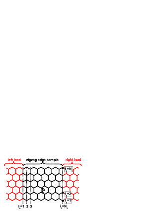
Figure 1: (color online) Geometry of the device for measuring the conductance of graphene nanoribbon. Two semi-infinite leads (red) are connected to the graphene nanoribbon sample with zigzag edges (black). The coordinate of each site is labelled as ($i_{x}$,$i_{y}$), where $1\leq i_{x}\leq N_{x}$ and $1\leq i_{y}\leq N_{y}$ are integers.

In this Letter, we perform systematic calculations to investigate the effect of the impurity potential range and its density on the conductance of graphene nanoribbon. The dependence of $\sigma(E_{F})$ displays four different types of behavior, corresponding to regimes with different length scales depending on the range and density of the impurities, which can be used as criterions in the experiments. Moreover, we demonstrate that the nonlinear dependence in the recent experiment Miao07 can also be explained when scattering due to the low density and long range impurities are accounted.

Model and Method.—We consider a two-terminal device to calculate the conductance, which includes a graphene nanoribbon and two leads with zigzag edges, as shown in Fig. 1, where the graphene sample is divided into $N_{x}$ vertical chains with $N_{y}$ sites in each chains. In this setting, the coordinate ($i_{x}$, $i_{y}$) ($1\leq i_{x}\leq N_{x}$, $1\leq i_{y}\leq N_{y}$) of each site is labelled. Two clean and semi-infinite leads are assumed to have the same type of lattice as the graphene sample 6 ; 14 to avoid additional scattering contribution from the mismatched interfaces between different types of lattices.

We describe graphene by the tight binding Hamiltonian for the $\pi$ orbital of carbon 17 ; Pe06n2

$$H=\sum_{i}\epsilon_{i}c_{i}^{\dagger}c_{i}+t\sum_{\langle i,j\rangle}(c_{i}^{\dagger}c_{j}+\text{H.c}),$$ (1)

where $c_{i}^{{\dagger}}$ ($c_{i}$) creates (annihilates) an electron on site $i$, $\varepsilon_{i}$ is the potential energy and $t$ ($\sim$2.7eV) is the hopping integral between the nearest neighbor carbon atoms with distance $a$ ($\sim$1.42Å). We use $t$ as the energy unit and $a$ as the length unit.

In the presence of disorder, $N_{i}$ impurities are randomly distributed among $N$ ($\equiv N_{x}\times N_{y}$) sites. The potential energy of the $i$-th site $\varepsilon_{i}$ at position $\mathbf{r}_{i}$ is induced by these impurities as 3 ; Wa07

$$\varepsilon_{i}(\mathbf{r}_{i})=\sum_{n=1}^{N_{i}}V_{n}\exp(-|\mathbf{r_{i}}-\mathbf{r_{n}}|^{2}/(2\xi^{2})),$$ (2)

where $\mathbf{r_{n}}$ is the position of the $n$-th impurity, $\xi$ represents the spatial range of the impurity potential, and the potential strength $V_{n}$ of the impurities is randomly distributed in the range $(-W/2,W/2)$, independently. The average distance between two impurities $R_{i}$ can be defined as $R_{i}\sim\sqrt{L_{x}L_{y}/N_{i}}$, where $L_{x(y)}$ is the length (width) of the rectangular sample. We shall show in the following that distinct interesting phenomena can be observed when the system is in the different regimes of these length scales that is determined by $L_{x(y)}$, $\xi$ and $R_{i}$.

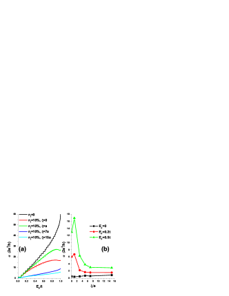
Figure 2: (color online) (a) Conductivity $\sigma$ of graphene nanoribbons with zigzag edges as a function of Fermi energy $E_{F}$ with different potential range $\xi$. (b) Conductivity $\sigma$ as a function of potential rnge $\xi$ at different Fermi energy $E_{F}$. $N_{x}=106$, $N_{y}=60$ ($L_{x}=90.9a$ and $L_{y}=89.0a$), $W=0.5t$ for both cases, where $t=2.7$eV and $a=1.42$nm. The conductivity is averaged over 100 random configurations for each curve.

In the framework of the non-equilibrium Green’s function method , the zero temperature conductance $G$ and density of states (DOS) $\rho$ of the sample at Fermi energy $E_{F}$ can be written as $G(E_{F})=\frac{2e^{2}}{h}\text{Tr}(\text{Im}\Sigma_{L}^{r}(E_{F})G^{r}(E_{F})\text{Im}\Sigma_{R}^{r}(E_{F})G^{a}(E_{F}))$ and $\rho(E_{F})=-\frac{1}{\pi}\text{Im}[\text{Tr}G^{r}(E_{F})]$, where $G^{r(a)}(E_{F})$ is the retarded (advanced) Green’s function, and $\Sigma_{L(R)}^{r(a)}$ is the retarded (advanced) self-energy due to the left (right) lead 4 ; 5 ; 6 ; BKN01 . The conductivity is related to the conductance by the geometric relation $\sigma=L_{x}G/L_{y}$.

In the clean limit, a self-consistent calculation for graphene in the Hartree approximation shows that, $\sigma\propto\sqrt{V_{g}}$ Ro07 . In this case, $\sigma\propto E_{F}$ 18 (also see Fig. 3 (a)). This leads to $E_{F}\simeq\alpha_{V_{g}}\sqrt{V_{g}}$, where $\alpha_{V_{g}}$ is a device-dependent prefactor, whose typical value $\sim 10^{-3}-10^{-2}$. This relation between $E_{f}$ and $V_{g}$ is valid even in the presence of disorder since it is a global response. Therefore, we can concentrate on the relation between $\sigma$ and $E_{f}$.

Figure 3: Conductivity of graphene nanoribbons with zigzag edges as a function of Fermi energy, with $N_{x}=106$, $N_{y}=60$ ($L_{x}=90.9a$ and $L_{y}=89a$), $W=0.5t$ at different $\xi$ and $n_{i}$. The conductivity is averaged over 100 random configurations for each curve. Note different $\sigma$ scalings in each regime. (a) Regime 1, no impurity. (b) Regime 2, short range impurities. (c) Regime 3, long range and low density impurities. (d) Regime 4, long range and high density impurities.

Results and Discussions.— Firstly, we investigate the effect of the potential range $\xi$ and density $n_{i}\equiv N_{i}/N$ of the impurities with fixed $W=0.5t$. Let us start by having a first glance at the effect of $\xi$. In Fig. 2 (a), we plot $\sigma(E_{F})$ with different $\xi$. A direct conclusion from this figure is that, in most regions of $E_{F}$, short range ($\xi=0,1a$) impurities can lead to a considerable decrease of conductivity, but long range ($\xi=7a,15a$) impurities will decrease the conductivity much further, in the case of same impurity density. In the experiments by Miao et al. the conductance is smaller than its ballistic value by a factor of 3–10, in the range of high $V_{g}$ Miao07 . This suggests that the samples used in these experiments must include long range impurities. Near the Dirac point $E_{F}=0$, this rapid variation breaks down, see Fig. 2 (b). The magnitude of $\sigma(E_{F}=0)$ is relatively universal ($\sim e^{2}/h$), compared to $\sigma$ at finite $E_{F}$. This is consistent with the experiment 7 . The linear dependence of $\sigma(E_{F})$ obtained in the mean field theory Zie06 is not entirely valid. Our numerical results indicate that $\sigma(E_{F})$ is a more complicated function that depends on the nature of disorder. To illustrate the physics, we focus on the conductivity $\sigma$ for graphene nanoribbons with zigzag edges for different $\xi$ and $n_{i}$, which can be seen in Fig. 3. All these behaviors can be classified into four typical regimes.

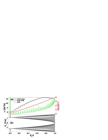
Figure 4: (color online) (a) Averaged conductivity of graphene ribbons with short range impurities (black) (Data are same with Fig.3 (b)) and long range impurities (red) (Data are same with Fig.3 (c)), and density of states of a clean ribbon with the same size (green, in arbitrary unit). (b) Band structure of a zigzag edge graphene nanoribbon with the same size. Note correspondences between these figures.

Regime 1, no impurity, $n_{i}=0$. When there is no impurities ($n_{i}=0$), $\sigma(E_{F})$ increases almost linearly except for small quantized plateaus due to finite size quantization in the transverse direction 18 , as shown in Fig. 3 (a). When the sample is large enough, these sub-structures due to finite size effect can be ignored, so $\sigma(E_{F})$ is linear, and $\sigma\sim\sqrt{V_{g}}$ according to $E_{F}\simeq\alpha_{V_{g}}\sqrt{V_{g}}$ Ro07 .

Regime 2, short range impurities, $\xi\lesssim a$. When short range impurities are present (Fig. 3 (b)), the first distinct feature is the sub-linear behavior of $\sigma(E_{F})$, especially in the high energy region. This anomaly can be understood as enhanced scattering due to large level broadening when DOS is large. In the coherent phase approximation without vertex corrections, the conductivity $\sigma$ of disordered system can be written as 20

$$\sigma=\frac{S_{F}}{8\pi^{2}}\frac{e^{2}v_{F}}{|\Sigma_{2}|},$$ (3)

where $S_{F}$ is the area of the Fermi sphere and $\Sigma_{2}$ is the imaginary part of self energy corresponding to the disorder scattering. The level broadening $|\Sigma_{2}|=\pi\rho N_{i}|V(q)|^{2}$, where $V(q)$ is the Fourier transform of impurity potential 20 . For a disordered nanoribbon, the van Hove singularity at $E=t$ of 2D graphene Naka96 ; 4 degenerates into a finite but still very sharp peak (see the green curve in Fig.4 (a)). Therefore, $\Sigma_{2}$ also has a sharp peak at this point, giving rise to a minimum of $\sigma$ as can be seen from (3). This minimum $\sigma$ at $E_{F}=t$ leads to a sub-linear $\sigma(E_{F})$ and sub-square root $\sigma(V_{g})$, according to the relation between $E_{F}$ and $V_{G}$ mentioned above.

Such level-broadening enhanced scattering also happens at the bottoms of sub-bands, where van Hove singularities emerge 13 ; QTD . Indeed, when disorder is not strong enough to smear these singularities out completely, a small dip can be observed at each sub-band bottom, as can be seen from Fig. 4 (a).

Variation of $n_{i}$ of short range impurities does not change the qualitative behavior of $\sigma(E_{F})$, but reduces the magnitude of $\sigma$ for a given $E_{F}$, when $\xi\sim 1$, as one expects. However, for extremely short range impurities ($\xi\sim 0$), we find that even the magnitude of $\sigma(E_{F})$ is quite independent of $n_{i}$ when $n_{i}>20\%$.

Regime 3. long range and low density impurities, $\xi\gg a$ and $\xi\lesssim R_{i}$. When the potential range $\xi$ increases further, interesting physics appears. As can be seen in Fig. 3 (c), the $\sigma(E_{F})$ curves resume their linear behavior in most energy regions (while the slope is much smaller as mentioned above). This manifests suppression of large momentum scattering due to the long range impurities.

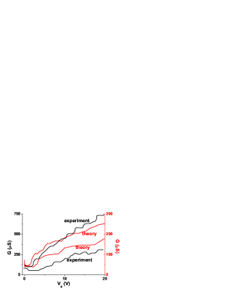
Figure 5: (color online) Conductivity $\sigma$ as a function of $V_{g}$: A qualitative comparison between theory and experiment. The black lines represent experimental results by Miao et al. Miao07 . The upper curve is for a larger sample and the lower curve is for a smaller sample. The red lines represent our numerical results. The upper curve: $N_{x}=120$, $N_{y}=110$, $\xi=4a$, $W=2t$; The lower curve: $N_{x}=72$, $N_{y}=80$, $\xi=4a$, $W=3t$. The conductivity is averaged over 50 random configurations for each curve.

Another notable nonlinear $\sigma(E_{F})$ can be observed near the Dirac point, where a wide dip appears. We find this happens within the energy region where the first sub-band is visible for a clean graphene (see Fig.4 (b)). For a smaller graphene sample, different sub-bands are more separated in energy than for a larger sample, giving rise to wider quantized conductance plateaus, and also a wider dip near the Dirac point, which is consistent with the experimental result Miao07 .

This wide dip can be understood as follows. As shown in Fig. 4 (b), the band structure near the Dirac point is composed of two branches of subbands, i.e., the upper band $+E(k_{x})>0$ and the lower band $-E(k_{x})<0$. These branches correspond to binding and antibinding states localized at different edges and sublattices Naka96 ; Ko06 . The wave functions of these edge states possess different signs according to two edges, sublattices and branches Hi03 . Long range impurities will (while short range ones will not) couple these edge states, giving rise to rather large scattering matrix elements between two valleys. When $E=0$, two branches and valleys degenerate, the magnitude of scattering matrix elements decreases since different signs of these edge states at $E=0$ making a larger possibility of canceling each other. This is verified by numerical calculations for scattering matrix elements.

Therefore, $\sigma(V_{g})$ behaves in a square root way in this regime, by noting $E_{F}\simeq\alpha_{V_{g}}\sqrt{V_{g}}$. In Fig. 5, we plot $\sigma(V_{g})$, setting $\alpha_{V_{g}}=10^{-3}$. A perfect quantitative fitting cannot be reached because the size of the sample in the experiments is the order of $N_{x,y}\sim 10^{3}$, which is well out of the capability of numerical calculations. But the qualitative features, i.e., sub-linearity and wide dip in the experiment (Fig. 5) can be clearly seen. Once again, we attribute this experimental result to the contribution of the low-density and long-range impurities.

Regime 4, long range and high density impurities, $\xi\gg a$ and $\xi\gg R_{i}$. In the case of low density impurities, the scatterings due to different impurities are independent. But when the density is sufficiently high, so that potential field induced by different impurities overlap, and multi-scattering dominates. This multi-scatterings have no obvious effect on the existence of the dip. While in the high energy region, the linear relation $\sigma(E_{F})$ breaks down and the curve degenerates into a square root like curve and $\sigma(V_{g})\sim\sqrt[4]{V_{g}}$ correspondingly, see Fig. 3 (d).

Finally, we discuss the energy scaling of the impurity potential $W$ considered to be fixed thus far. In our calculations $W$ is much larger than the level spacing of sub-bands. The opposite limit has been investigated recently, and a perfectly conducting channel was found Wa07 .

Conclusions.—As a summary, we numerically investigate the transport properties of graphene nanoribbons in the presence of the impurities with different density and potential range. In the Fermi energy region of focus, four typical types of behavior can appear from the unconventional electronic structures in zigzag graphene nanoribbons, which can be tested by future experiments. The third regime for the low density and long range impurities can be used to explain the nonlinearity of $\sigma(V_{g})$ in a recent experiment Miao07 .

We acknowledge useful discussions with Professors C. N. Lau, S. C. Zhang, Q. Niu, C. W. J. Beenakker, J. R. Shi and Q. F. Sun. This work was supported by NSF of China under grant 90406017, 60525417, 10610335, the NKBRSF of China under Grant 2005CB724508 and 2006CB921400. X. C. Xie is supported by US-DOE and US-NSF.

References

- [1] K. S. Novoselov et al., Science 306, 666 (2004); Nature 438, 197 (2005); Y. Zhang et al., Nature 438, 201 (2005).
- [2] K. Ziegler, Phys. Rev. Lett. 80, 3113 (1998).
- [3] D. V. Khveshchenko, Phys. Rev. Lett. 97, 036802 (2006).
- [4] I. L. Aleiner et al., Phys. Rev. Lett. 97, 236801 (2006).
- [5] A. Altland, Phys. Rev. Lett. 97, 236802 (2006).
- [6] S. V. Morozov et al., Phys. Rev. Lett. 97, 016801 (2006).
- [7] X. Wu et al., Phys. Rev. Lett. 98, 136801 (2007).
- [8] B. Huard et al., Phys. Rev. Lett. 98, 236803 (2007).
- [9] G. M. Rutter et al., Science 317, 219 (2007).
- [10] N. H. Shon et al., J. Phys. Soc. Jap. 67, 2421 (1998).
- [11] H. Suzuura et al., Phys. Rev. Lett. 89, 266603 (2002).
- [12] A. Rycerz et al., cond-mat/0612446 (2006).
- [13] A. F. Morpurgo et al., Phys. Rev. Lett. 97, 196804 (2006).
- [14] K. Nomura et al., Phys. Rev. Lett. 98, 076602 (2007).
- [15] E. H. Hwang et al., Phys. Rev. Lett. 98, 186806 (2007).
- [16] P. M. Ostrovsky et al., Phys. Rev. Lett. 98, 256801 (2007).
- [17] K. Wakabayashi et al., Phys. Rev. Lett. 99, 036601 (2007).
- [18] F. Miao et al., to appear in Science. see also: cond-mat/0703052 (2007).
- [19] J. Zhang et al., J. Chem. Phys. 120, 7733 (2004).
- [20] J. Tworzydło et al., Phys. Rev. Lett. 96, 246802 (2006).
- [21] R. Saito et al., Physical Properties of Carbon Nanotubes (Imperial College Press, London. 1998).
- [22] N. M. R. Peres et al., Phys. Rev. B 73, 125411 (2006).
- [23] S. Datta, Electronic Transport in Mesoscopic Systems (Canmbridge University Press, Cambridge, U.K., 1995).
- [24] D. H. Lee et al., Phys. Rev. B 23, 4997 (1981).
- [25] B. K. Nikolić, Phys. Rev. B 64, 165303 (2001).
- [26] J. Fernández-Rossier et al., Phys. Rev. B 75, 205441 (2007).
- [27] N. M. R. Peres et al., Phys. Rev. B 73, 195411 (2006).
- [28] K. Ziegler, Phys. Rev. Lett. 97, 266802 (2006).
- [29] E. N. Economou, Green’s Functions in Quantum Physics, 3rd Edition (Springer-Verlag. 2006).
- [30] S. DasSarma et al., Phys. Rev. B 35, 9875 (1987).
- [31] T. Dittrich et al., Quantum Transport and Dissipation (Wiley-VCH. 1998).
- [32] K. Nakada et al., Phys. Rev. B 54, 17954 (1996); K. Wakabayashi et al., ibid. 64, 125428 (2001).
- [33] Y. Kobayashi et al., Phys. Rev. B 71, 193406 (2005); Y. Niimi et al., ibid. 73, 085421 (2006).
- [34] T. Hikihara et al., Phys. Rev. B 68, 035432 (2003).