Neutrino oscillations in matter and in twisting magnetic fields

Abstract

We find the solution to the Dirac equation for a massive neutrino with a magnetic moment propagating in background matter and interacting with the twisting magnetic field. In frames of the relativistic quantum mechanics approach to the description of neutrino evolution we use the obtained solution to derive neutrino wave functions satisfying the given initial condition. We apply the results to the analysis of neutrino spin oscillations in matter under the influence of the twisting magnetic field. Then on the basis of the yielded results we describe spin-flavor oscillations of Dirac neutrinos that mix and have non-vanishing matrix of magnetic moments. We again formulate the initial condition problem, derive neutrinos wave functions and calculate the transition probabilities for different magnetic moments matrices. The consistency of the obtained results with the quantum mechanical treatment of spin-flavor oscillations is discussed. We also consider several applications to astrophysical and cosmological neutrinos.

I Introduction

Neutrino conversions from one flavor to another combined with the change of the particle helicity, e.g. $\nu_{e}^{\mathrm{L}}\leftrightarrow\nu_{\mu}^{\mathrm{R}}$, are usually called neutrino spin-flavor oscillations (see Ref. qmSFO ). This neutrino oscillations scenario is important since it could be the explanation of the time variability of the solar neutrino flux (see, e.g., Ref. solarnu ). Massive flavor neutrinos are known to mix and can have non-zero magnetic moments. The influence of the strong magnetic field with the realistic profile could lead to the spin-flavor oscillations of solar neutrinos (see, e.g., Ref. realisticB ). Moreover, studying neutrino spin-flavor oscillations happening inside the Sun, one will be able to discriminate between different solar models PicPulAndBarMan07 . However it was found out in Ref. smallcontr that neutrino spin-flavor oscillations in solar magnetic fields give a sub-dominant contribution to the total conversion of solar neutrinos.

In this paper we study neutrino spin and spin-flavor oscillations in matter and in an external magnetic field. We suppose that a neutrino is a Dirac particle with a non-zero magnetic moment. It should be mentioned that in spite of the recent claims of the experimental confirmation that neutrinos are Majorana particles KleKriDieChk04 , the question about the nature of neutrinos is still open EllEng04 . The possibility to distinguish between Dirac and Majorana particles in the partially polarized solar neutrino flux, due to the spin-flavor precession, was examined in Ref. Sem97 .

To describe the evolution of the neutrino system we apply the technique based on the relativistic quantum mechanics. We start from the exact solution to the Dirac equation in an external field and then derive the neutrino wave functions satisfying the given initial condition. We used this method to describe neutrino flavor oscillations in vacuum FOvac , in background matter Dvo06EPJC and spin-flavor oscillations in an external magnetic field DvoMaa07 . Note that neutrino spin-flavor oscillations in electromagnetic fields of various configurations were examined in Refs. emfields ; Dvo07YadFiz ; twisting using the standard quantum mechanical approach.

In Sec. II we find the solution to the Dirac equation for a neutrino propagating in background matter and interacting with the twisting magnetic field. Then we formulate the initial condition problem and receive the transition probability for spin oscillations in the given external fields. The standard quantum mechanical transition probability formula is re-derived and the conditions of its validity are analyzed. In Sec. III we apply the obtained Dirac equation solutions to the description of neutrino spin-flavor oscillations in the twisting magnetic field. First we discuss magnetic moment matrices of neutrinos in flavor and mass eigenstates bases. Then we solve the initial condition problem in two different cases of the magnetic moments matrix in the mass eigenstates basis with (i) great diagonal elements and (ii) great non-diagonal elements. Note that the analogous magnetic moments matrices were discussed in Ref. DvoMaa07 . We get neutrinos wave functions and calculate transition probabilities for processes like $\nu_{\beta}^{\mathrm{L}}\xrightarrow{B}\nu_{\alpha}^{\mathrm{R}}$. The consistency of the Dirac-Pauli equation approach with the standard quantum mechanical treatment of spin-flavor oscillations, based on the Schrödinger evolution equation, is considered in Sec. IV. Then in Sec. V we present some applications and finally we summarize our results in Sec. VI.

II Neutrino spin oscillations in matter and in a twisting magnetic field

In this section we obtain the exact solution to the Dirac-Pauli equation for a neutrino interacting with background matter and a twisting magnetic field and discuss spin oscillations of a single Dirac neutrino in the given external fields.

A neutrino is taken to have the non-zero mass $m$ and the magnetic moment $\mu$. The Lagrangian for this system has the form,

$$\mathcal{L}=\bar{\nu}(\mathrm{i}\gamma^{\mu}\partial_{\mu}-m)\nu-\bar{\nu}\gamma_{\mu}^{\mathrm{L}}\nu f^{\mu}-\frac{\mu}{2}\bar{\nu}\sigma_{\mu\nu}\nu F^{\mu\nu},$$ (1)

where $\gamma_{\mu}^{\mathrm{L}}=\gamma_{\mu}(1+\gamma^{5})/2$, $\sigma_{\mu\nu}=(\mathrm{i}/2)(\gamma_{\mu}\gamma_{\nu}-\gamma_{\nu}\gamma_{\mu})$ and $F_{\mu\nu}=(\mathbf{E},\mathbf{B})$ is the electromagnetic field tensor. In the following we will discuss the situation when only magnetic field $\mathbf{B}$ is presented, i.e. $\mathbf{E}=0$. The neutrino interaction with matter is characterized by the four vector $f^{\mu}$. For the non-moving and unpolarized matter one can take that the spatial components of the vector $f^{\mu}$ are zero, i.e. $\mathbf{f}=0$. If, for instance, we consider an electron neutrino propagating in matter, which consists of electrons, protons and neutrons, we obtain for the time component, $f^{0}$, of the vector $f^{\mu}$ (see, e.g., Ref. DvoStu02JHEP ),

$$f^{0}= \sqrt{2}G_{\mathrm{F}}\sum_{f=e,p,n}n_{f}q_{f},$$

$$q_{f}= (I_{3\mathrm{L}}^{(f)}-2Q^{(f)}\sin^{2}\theta_{W}+\delta_{ef}),$$ (2)

where $n_{f}$ is the number density of background particles, $I_{3\mathrm{L}}^{(f)}$ is the third isospin component of the matter fermion $f$, $Q^{(f)}$ is its electric charge, $\theta_{W}$ is the Weinberg angle and $G_{\mathrm{F}}$ is the Fermi constant.

It should be noted that Eqs. (1) and (II) constitute the phenomenological model studied in the present paper. These expressions are valid in a relatively weak external magnetic field. For example, one has to take into account the spatial components of the vector $f^{\mu}$ if we describe neutrino propagation in background matter composed of electrons under the influence of a very strong magnetic field with $\sqrt{|\mathbf{B}|}\gg\max(m_{e},T,\mathfrak{M},|\mathbf{p}|)$, where $m_{e}$ is the electron mass, $T$ is the temperature of background matter, $\mathfrak{M}$ is its chemical potential and $\mathbf{p}$ is the neutrino momentum. This situation was analyzed in Ref. EliFerInc04 .

Using Eq. (1) one writes down the Dirac equation which accounts for the neutrino interaction with matter and magnetic field,

$$\mathrm{i}\dot{\nu}= \mathcal{H}\nu,$$

$$\mathcal{H}= (\bm{\alpha}\hat{\mathbf{p}})+\beta m-\mu\beta(\bm{\Sigma}\mathbf{B})+f^{0}(1+\gamma^{5})/2,$$ (3)

where $\bm{\alpha}=\gamma^{0}\bm{\gamma}$, $\beta=\gamma^{0}$ and $\bm{\Sigma}=\gamma^{0}\gamma^{5}\bm{\gamma}$ are the Dirac matrices. Let us discuss the case of the twisting magnetic field, $\mathbf{B}=B(0,\sin\omega x,\cos\omega x)$, where $\omega$ is the frequency of the magnetic field rotation. Sometimes it is called the spiral undulator magnetic field. Note that neutrino oscillations in twisting magnetic fields in frames of the quantum mechanical approach were studied in Ref. twisting .

We notice that the Hamiltonian $\mathcal{H}$ in Eq. (II) depends on neither $y$ nor $z$ coordinates. Therefore we assume that the wave function depends on these coordinates exponentially, $\nu\sim\exp(\mathrm{i}p_{y}y+\mathrm{i}p_{z}z)$, where $p_{y}$ and $p_{z}$ are constant values. Then for simplicity one can take that $p_{y}=p_{z}=0$. It means that a neutrino moves along the undulator axis. Let us express the neutrino wave function in terms of the two component spinors, $\nu^{\mathrm{T}}=(\varphi,\chi)$. On the basis of Eq. (II) we receive equations for the two component spinors,

$$\mathrm{i}\dot{\varphi}= (m-\mu(\bm{\sigma}_{\perp{}}\mathbf{B})+f^{0}/2)\varphi+(\sigma_{1}\hat{p}_{x}-f^{0}/2)\chi,$$

$$\mathrm{i}\dot{\chi}= (-m+\mu(\bm{\sigma}_{\perp{}}\mathbf{B})+f^{0}/2)\chi+(\sigma_{1}\hat{p}_{x}-f^{0}/2)\varphi,$$ (4)

where $\hat{p}_{x}=-\mathrm{i}\partial_{x}$ and $\bm{\sigma}_{\perp{}}=(\sigma_{2},\sigma_{3})$.

Now we replace the neutrino wave function $\nu$ with the new one, $\nu\to\tilde{\nu}=\mathcal{U}^{\dagger}\nu$, where $\mathcal{U}=\mathrm{diag}(\mathfrak{U},\mathfrak{U})$ and $\mathfrak{U}=\cos(\omega x/2)+\mathrm{i}\sigma_{1}\sin(\omega x/2)$. Then we again express the new wave function using the two component spinors, $\tilde{\nu}^{\mathrm{T}}=(\xi,\eta)$, with $\varphi=\mathfrak{U}\xi$ and $\chi=\mathfrak{U}\eta$. With help of the following properties of the matrix $\mathfrak{U}$: $\mathfrak{U}^{\dagger}(\bm{\sigma}_{\perp{}}\mathbf{B})\mathfrak{U}=\sigma_{3}B$, $\mathrm{d}\mathfrak{U}/\mathrm{d}x=\mathrm{i}\sigma_{1}\omega\mathfrak{U}/2$ and $\mathfrak{U}^{\dagger}\sigma_{1}\mathfrak{U}=\sigma_{1}$, as well as using Eq. (II) we arrive to the equations for the new two component spinors,

$$\mathrm{i}\dot{\xi}= (m-\mu B\sigma_{3}+f^{0}/2)\xi$$

$$+[(\omega-f^{0})/2+\sigma_{1}\hat{p}_{x}]\eta,$$

$$\mathrm{i}\dot{\eta}= (-m+\mu B\sigma_{3}+f^{0}/2)\eta$$

$$+[(\omega-f^{0})/2+\sigma_{1}\hat{p}_{x}]\xi.$$ (5)

We notice that Eq. (II) do not contain the dependence on $x$ coordinate. Thus one gets that the new wave function depends on $x$ as $\tilde{\nu}\sim\exp(\mathrm{i}px)$, where $p$ is a constant value, the analog of the particle momentum. It means that we can replace $\hat{p}_{x}\to p$ in Eq. (II).

We look for stationary solutions to Eq. (II), i.e. $\tilde{\nu}\sim\exp(-\mathrm{i}Et)$. Supposing that this equation has a non-trivial solution we receive the energy levels in the form, $E=f^{0}/2\pm E^{(\zeta)}$. The function $E^{(\zeta)}$ depends on the momentum and the characteristics on the external fields as

$$E^{(\zeta)}=\sqrt{\mathcal{M}^{2}+m^{2}+p^{2}-2\zeta R^{2}},$$ (6)

where $R^{2}=\sqrt{p^{2}\mathcal{M}^{2}+(\mu B)^{2}m^{2}}$ and $\mathcal{M}=\sqrt{(\mu B)^{2}+(\omega-f^{0})^{2}/4}$. In Eq. (6) $\zeta=\pm 1$ is the discrete quantum number.

Using energy spectrum (6) we can reproduce the results of the previous works where the Dirac equation for a neutrino interacting with various external fields was solved. Namely,

• neutrino interaction with a constant transversal magnetic field (see, e.g., Ref. DvoMaa07 ). This situation corresponds to $\omega=0$ and $f^{0}=0$. Using Eq. (6) we get $E=\pm\left(\sqrt{m^{2}+p^{2}}-\zeta\mu B\right)$ that coincides with the energy spectrum used in Ref. DvoMaa07 ;

• neutrino interaction with background matter (see Ref. matterQFT ). This case corresponds to $\omega=0$ and $B=0$. With help of Eq. (6) we receive that $E=f^{0}/2\pm\sqrt{(p-\zeta f^{0}/2)^{2}+m^{2}}$ that coincides with the results of Ref. matterQFT .

Note that, if we set $\omega=0$ and $B\neq 0$ in Eq. (6), we arrive to the case of a neutrino propagating in background matter under the influence of a constant transversal magnetic field.

The basis spinors $u^{(\zeta)}$ and $v^{(\zeta)}$ corresponding to the signs $\pm{}$ in the dispersion relation can be found from Eq. (II). The general expressions for these spinors, which account for the particle mass exactly, are rather complicated. Therefore we present here the basis spinors for a relativistic neutrino with $(m/E)\ll 1$,

$$u^{(\zeta)}= \frac{1}{2\sqrt{2\mathcal{M}(\mathcal{M}+\varDelta)}}\begin{pmatrix}\mu B+\zeta\mathcal{M}+\varDelta\\ \mu B-\zeta\mathcal{M}-\varDelta\\ \mu B-\zeta\mathcal{M}-\varDelta\\ \mu B+\zeta\mathcal{M}+\varDelta\ \end{pmatrix},$$

$$v^{(\zeta)}= \frac{1}{2\sqrt{2\mathcal{M}(\mathcal{M}-\varDelta)}}\begin{pmatrix}\mathcal{M}-\varDelta-\zeta\mu B\\ \mathcal{M}-\varDelta+\zeta\mu B\\ \varDelta-\mathcal{M}-\zeta\mu B\\ \varDelta-\mathcal{M}+\zeta\mu B\ \end{pmatrix},$$ (7)

where $\varDelta=(\omega-f^{0})/2$. Note that the basis spinors in Eq. (II) satisfy the orthonormality conditions,

$$u^{(\zeta){\dagger}}u^{(\zeta^{\prime})}=v^{(\zeta){\dagger}}v^{(\zeta^{\prime})}=\delta_{\zeta\zeta^{\prime}},\quad u^{(\zeta){\dagger}}v^{(\zeta^{\prime})}=0.$$ (8)

II.1 Neutrino evolution in matter under the influence of a twisting magnetic field

Using the approach developed in our previous works FOvac ; Dvo06EPJC ; DvoMaa07 we can formulate the initial condition problem for the system in question. For the given initial wave function $\nu(x,0)$ one should find the wave function $\nu(x,t)$ at subsequent moments of time, while a particle propagates in the external fields. This wave function has the form (see Refs. FOvac ; Dvo06EPJC ; DvoMaa07 ),

$$\nu(x,t)=\mathcal{U}(x)e^{-\mathrm{i}f^{0}t/2}\int_{-\infty}^{+\infty}\frac{\mathrm{d}p}{2\pi}e^{\mathrm{i}px}S(p,t)\tilde{\nu}(p,0),$$ (9)

where

$$\tilde{\nu}(p,0)=\int_{-\infty}^{+\infty}\mathrm{d}xe^{-\mathrm{i}px}\mathcal{U}^{\dagger}(x)\nu(x,0),$$ (10)

is the Fourier transform of the initial condition for the fermion $\tilde{\nu}$ and

$$S(p,t)= \sum_{\zeta=\pm 1}\bigg{[}\left(u^{(\zeta)}\otimes u^{(\zeta){\dagger}}\right)\exp{(-\mathrm{i}E^{(\zeta)}t)}$$

$$+\left(v^{(\zeta)}\otimes v^{(\zeta){\dagger}}\right)\exp{(+\mathrm{i}E^{(\zeta)}t)}\bigg{]},$$ (11)

is the analog for the Pauli-Jourdan function for a spinor field interacting with matter and a twisting magnetic field. The basis spinors $u^{(\zeta)}$ and $v^{(\zeta)}$ are presented in Eq. (II). To derive Eqs. (9)-(II.1) we use orthonormality of the basis spinors (8).

Let us suppose that initially a neutrino is in the state with the following wave function: $\nu(x,0)=e^{\mathrm{i}kx}\xi_{0}$, where $\xi_{0}^{\mathrm{T}}=(1/2)(1,-1,-1,1)$. It is possible to check that $(1/2)(1-\Sigma_{1})\xi_{0}=\xi_{0}$. Hence, the spinor $\nu(x,0)$ describes a particle propagating along the $x$-axis, with its spin directed opposite to the $x$-axis, i.e. a left-handed neutrino. Analogous initial condition was adopted in Refs. FOvac ; Dvo06EPJC ; DvoMaa07 where neutrino flavor and spin-flavor oscillations were studied.

Using Eq. (10) we find that $\tilde{\nu}(p,0)=2\pi\delta(p-k-\omega/2)\xi_{0}$. It is interesting to note that the following identity is satisfied: $\left(v^{(\zeta)}\otimes v^{(\zeta){\dagger}}\right)\xi_{0}=0$. Therefore no particles with ”negative” energies appear in neutrino interacting with considered external fields. Using Eqs. (II) and (9)-(II.1) as well as the chosen initial condition we arrive to the right-polarized component of the final wave function,

$$\nu^{\mathrm{R}}(x,t)= \frac{1}{2}(1+\Sigma_{1})\nu(x,t)$$ (12)

$$= \exp[\mathrm{i}(k+\omega)x-\mathrm{i}f^{0}t/2]$$

$$\times\frac{\mu B}{2\mathcal{M}}\left.\left(e^{-\mathrm{i}E^{+{}}t}-e^{-\mathrm{i}E^{-{}}t}\right)\right|_{p=k+\omega/2}\kappa_{0},$$

where $\kappa_{0}^{\mathrm{T}}=(1/2)(1,1,1,1)$.

Supposing that initially no right-polarized particles are present and with help of Eq. (12) we calculate the transition probability for the process $\nu^{\mathrm{L}}\to\nu^{\mathrm{R}}$,

$$P_{\nu^{\mathrm{L}}\to\nu^{\mathrm{R}}}(t)= \frac{(\mu B)^{2}}{(\mu B)^{2}+\varDelta^{2}}$$

$$\times\sin^{2}\left.\left(\frac{E^{+{}}-E^{-{}}}{2}t\right)\right|_{p=k+\omega/2}.$$ (13)

It can be seen from Eq. (II.1) that the resonance in neutrino spin oscillations occurs when $\varDelta\to 0$. One finds from Eq. (6) that $(E^{+{}}-E^{-{}})/2=-\mu B$ at $\varDelta=0$. Therefore the resonance transition probability is always $P_{\mathrm{res}}(t)=\sin^{2}(\mu Bt)$.

To analyze Eq. (II.1) we introduce the group velocity,

$$\mathcal{V}^{(\zeta)}=\frac{\partial E}{\partial p}=\frac{p}{E^{(\zeta)}}\left(1-\zeta\frac{\mathcal{M}^{2}}{R^{2}}\right).$$ (14)

Now we can distinguish three different cases.

1. First we suppose that $p=0$. This situation can happen if $k=-\omega/2$. With help of Eq. (6) we obtain that the energy levels are $E^{(\zeta)}=\sqrt{(m-\zeta\mu B)^{2}+\varDelta^{2}}$. Using Eq. (14) we receive that the group velocity vanishes, $\mathcal{V}^{(\zeta)}=0$. It means that the neutrino is captured by the twisting magnetic field.

2. Now we assume that $p=\pm\mathcal{M}$, with $p\neq 0$. For the definiteness we discuss the situation when $p=\mathcal{M}$ since the case $p=-\mathcal{M}$ can be considered analogously. The energies corresponding to different values of $\zeta$ are

   $$E^{+{}}= m\sqrt{1-\frac{(\mu B)^{2}}{\mathcal{M}^{2}}+\frac{(\mu B)^{4}m^{2}}{2\mathcal{M}^{6}}},$$

   $$E^{-{}}= 2\mathcal{M}\left(1+\frac{m^{2}}{8\mathcal{M}^{2}}\left[1+\frac{(\mu B)^{2}}{\mathcal{M}^{2}}\right]\right).$$ (15)

   Using Eq. (14) one can compute the group velocities,

   $$\mathcal{V}^{+{}}= \frac{(\mu B)^{2}m}{2\mathcal{M}^{3}}\left[1-\frac{(\mu B)^{2}}{\mathcal{M}^{2}}+\frac{(\mu B)^{4}m^{2}}{2\mathcal{M}^{6}}\right]^{-1/2},$$

   $$\mathcal{V}^{-{}}= 1-\frac{m^{2}}{8\mathcal{M}^{2}}\left[1+3\frac{(\mu B)^{2}}{\mathcal{M}^{2}}\right].$$ (16)

   In Eqs. (2) and (2) we suppose that $m\ll\mathcal{M}$. On the basis of Eqs. (2) and (2) we get the resonance energies ($\varDelta\to 0$),

   $$E^{+{}}_{\mathrm{res}}\to \frac{m^{2}}{\sqrt{2}\mu B},$$

   $$E^{-{}}_{\mathrm{res}}\to 2\mu B\left[1+\frac{m^{2}}{4(\mu B)^{2}}\right],$$ (17)

   and group velocities

   $$\mathcal{V}^{+{}}_{\mathrm{res}}\to\frac{1}{\sqrt{2}},\quad\mathcal{V}^{-{}}_{\mathrm{res}}\to 1-\frac{m^{2}}{2(\mu B)^{2}}.$$ (18)

   It should be noted that group velocities are always less than one, $\mathcal{V}^{\pm{}}<1$ [see, e.g., Eq. (18)].

3. The last situation is realized when $p\neq\pm\mathcal{M}$ and $p\neq 0$. The energies in this case have the form,

   $$E^{(\zeta)}= p-\zeta\mathcal{M}$$

   $$+\frac{m^{2}}{2(p-\zeta\mathcal{M})}\left[1-\zeta\frac{(\mu B)^{2}}{\mathcal{M}p}\right].$$ (19)

   The expression for the transition probability (II.1) is now rewritten in the following way:

   $$P(t)= \frac{(\mu B)^{2}}{(\mu B)^{2}+\varDelta^{2}}$$

   $$\times\sin^{2}\left(\sqrt{(\mu B)^{2}+\varDelta^{2}}t\right).$$ (20)

   Note that transition probability expressions for spin oscillations derived earlier (see, e.g., Ref. twisting ) coincide with Eq. (3) which is valid only if $p\neq\pm\mathcal{M}$ and $p\neq 0$.

It should be noted that the ”non-standard” regimes in neutrino spin oscillations described in items 1 and 2 are likely to be realized for neutrinos with small initial momenta (see also Sec. V below).

III Neutrino spin-flavor oscillations in a twisting magnetic field

Now we apply the results of the previous section to the description of neutrino spin-flavor oscillations in a twisting magnetic field. Let us study the evolution of two Dirac neutrinos $(\nu_{\alpha},\nu_{\beta})$ that mix and interact with the external electromagnetic field $F_{\mu\nu}$. The Lagrangian for this system has the form

$$\mathcal{L}(\nu_{\alpha},\nu_{\beta})= \sum_{\lambda=\alpha,\beta}\bar{\nu}_{\lambda}\mathrm{i}\gamma^{\mu}\partial_{\mu}\nu_{\lambda}-\sum_{\lambda\lambda^{\prime}=\alpha,\beta}\bigg{[}m_{\lambda\lambda^{\prime}}\bar{\nu}_{\lambda}\nu_{\lambda^{\prime}}$$

$$+\frac{1}{2}M_{\lambda\lambda^{\prime}}\bar{\nu}_{\lambda}\sigma_{\mu\nu}\nu_{\lambda^{\prime}}F^{\mu\nu}\bigg{]},$$ (21)

Here $(m_{\lambda\lambda^{\prime}})$ and $(M_{\lambda\lambda^{\prime}})$ are the mass and the magnetic moments matrices that are generally independent. By definition these matrices are intoduced in the flavor eigenstates basis. The electromagnetic field is taken to have the same configuration as in Sec. II.

To analyze the dynamics of the system we again set the initial condition by specifying the initial wave functions of the flavor neutrinos $\nu_{\lambda}$ and then analytically determine the field distributions at following moments of time. We assume that the initial condition is

$$\nu_{\alpha}(x,0)=0,\quad\nu_{\beta}(x,0)=\xi(x),$$ (22)

where $\xi(x)$ is a function to be specified. One of the possible choices for the initial condition for $\nu_{\beta}$ is the plane wave field distribution, $\xi(x)=e^{\mathrm{i}kx}\xi_{0}$ (see Refs. FOvac ; Dvo06EPJC ; DvoMaa07 ). If we study ultrarelativistic initial particles, we can choose the spinor $\xi_{0}$ as in Sec. II, i.e. in the following form: $\xi_{0}^{\mathrm{T}}=(1/2)(1,-1,-1,1)$.

In order to eliminate the vacuum mixing term in Eq. (III), i.e. to diagonalize the mass matrix, we introduce a new basis of the wave functions, the mass eigenstate basis $\psi_{a}$, $a=1,2$, obtained from the original flavor basis $\nu_{\lambda}$ through the unitary transformation

$$\nu_{\lambda}=\sum_{a=1,2}U_{\lambda a}\psi_{a},$$ (23)

where the matrix $({U}_{\lambda a})$ is parametrized in terms of a mixing angle $\theta$ as usual

$$({U}_{\lambda a})=\begin{pmatrix}\cos\theta&-\sin\theta\\ \sin\theta&\cos\theta\ \end{pmatrix}.$$ (24)

The Lagrangian (III) rewritten in terms of the fields $\psi_{a}$ takes the form

$$\mathcal{L}(\psi_{1},\psi_{2})= \sum_{a=1,2}\mathcal{L}_{0}(\psi_{a})$$

$$-\frac{1}{2}\sum_{ab=1,2}\mu_{ab}\bar{\psi}_{a}\sigma_{\mu\nu}\psi_{b}F^{\mu\nu},$$ (25)

where $\mathcal{L}_{0}(\psi_{a})=\bar{\psi}_{a}(\mathrm{i}\gamma^{\mu}\partial_{\mu}-m_{a})\psi_{a}$ is the Lagrangian for the free fermion $\psi_{a}$ with the mass $m_{a}$ and

$$\mu_{ab}=\sum_{\lambda\lambda^{\prime}=\alpha,\beta}U^{-1}_{a\lambda}{M}_{\lambda\lambda^{\prime}}U_{\lambda^{\prime}b},$$ (26)

is the magnetic moment matrix presented in the mass eigenstates basis. Using Eqs. (22)-(24) the initial conditions for the fermions $\psi_{a}$ become

$$\psi_{1}(x,0)=\sin\theta\xi(x),\quad\psi_{2}(x,0)=\cos\theta\xi(x).$$ (27)

For the given configuration of the electric and magnetic fields we write down the Dirac-Pauli equation for $\psi_{a}$, resulting from Eq. (III), as follows:

$$\mathrm{i}\dot{\psi}_{a}=\mathcal{H}_{a}\psi_{a}+V\psi_{b},\quad a,b=1,2,\quad a\neq b,$$ (28)

where $\mathcal{H}_{a}=(\bm{\alpha}\mathbf{p})+\beta m_{a}-\mu_{a}\beta(\bm{\Sigma}\mathbf{B})$ is the Hamiltonian for the particle $\psi_{a}$ accounting for the magnetic field, $V=-\mu\beta(\bm{\Sigma}\mathbf{B})$ describes the interaction of the transition magnetic moment with the external magnetic field, $\mu_{a}=\mu_{aa}$, and $\mu=\mu_{12}=\mu_{21}$ are elements of the matrix $({\mu}_{ab})$.

To find the general solution to Eq. (28) we follow the method used in Sec. II and introduce the new wave functions $\tilde{\psi}_{a}=\mathcal{U}^{\dagger}\psi_{a}$. All the calculations are identical to those made in Sec. II. Therefore we present the final result for the wave functions $\tilde{\psi}_{a}$,

$$\tilde{\psi}_{a}(x,t)= \int_{-\infty}^{+\infty}\frac{\mathrm{d}p}{\sqrt{2\pi}}e^{\mathrm{i}px}$$

$$\times\sum_{\zeta=\pm 1}\Big{[}a_{a}^{(\zeta)}(t)u_{a}^{(\zeta)}\exp{(-\mathrm{i}E_{a}^{(\zeta)}t)}$$

$$+b_{a}^{(\zeta)}(t)v_{a}^{(\zeta)}\exp{(+\mathrm{i}E_{a}^{(\zeta)}t)}\Big{]},$$ (29)

where the energy levels $E_{a}^{(\zeta)}$ are

$$E_{a}^{(\zeta)}=\sqrt{\mathcal{M}_{a}^{2}+m_{a}^{2}+p^{2}-2\zeta R_{a}^{2}}.$$ (30)

Here [see Eq. (6)]

$$R_{a}^{2}= \sqrt{p^{2}\mathcal{M}_{a}^{2}+(\mu_{a}B)^{2}m_{a}^{2}},$$

$$\mathcal{M}_{a}= \sqrt{(\mu_{a}B)^{2}+\omega^{2}/4}.$$ (31)

The basis spinors $u_{a}^{(\zeta)}$ and $v_{a}^{(\zeta)}$ can be obtained from Eq. (II) by the following replacement: $\mu\to\mu_{a}$, $\mathcal{M}\to\mathcal{M}_{a}$ and $f^{0}\to 0$. Our main goal is to determine the non-operator coefficients $a_{a}^{(\zeta)}$ and $b_{a}^{(\zeta)}$ so that to satisfy both the initial condition (27) and the evolution equation (28). Generally the coefficients $a_{a}^{(\zeta)}(t)$ and $b_{a}^{(\zeta)}(t)$ are functions of time.

III.1 Spin-flavor oscillations in case of diagonal magnetic moments

In this section we suppose that magnetic moments matrix in the mass eigenstates basis is close to diagonal, i.e. $\mu_{a}\gg\mu$. This case should be analyzed with help of the perturbation theory. We expand the wave functions $\tilde{\psi}_{a}$ in a series

$$\tilde{\psi}_{a}(x,t)=\tilde{\psi}^{(0)}(x,t)+\tilde{\psi}_{a}^{(1)}(x,t)+\dots,$$ (32)

where $\tilde{\psi}^{(0)}(x,t)$ corresponds to the solution of Eq. (III) when we neglect the potential $V$ there. The function $\tilde{\psi}_{a}^{(1)}(x,t)$ is linear in the transition magnetic moment $\mu$ etc. We omit terms of higher order in $\mu$ in Eq. (32). They can be also accounted for but the corresponding calculations arrear to be cumbersome in the general case.

Using orthonormality conditions of the basis spinors [see also Eq. (8)],

$$u_{a}^{(\zeta){\dagger}}u_{a}^{(\zeta^{\prime})}=v_{a}^{(\zeta){\dagger}}v_{a}^{(\zeta^{\prime})}=\delta_{\zeta\zeta^{\prime}},\quad u_{a}^{(\zeta){\dagger}}v_{a}^{(\zeta^{\prime})}=0,$$

and the results of our previous work DvoMaa07 (see also Sec. II) we can receive from Eq. (III) the expression for the zero order (in $\mu$) wave functions $\psi_{a}^{(0)}$, which correspond to the first term in Eq. (32),

$$\psi_{a}^{(0)}(x,t)=\mathcal{U}(x)\int_{-\infty}^{+\infty}\frac{\mathrm{d}p}{2\pi}e^{\mathrm{i}px}S_{a}(p,t)\tilde{\psi}_{a}(p,0).$$ (33)

where

$$\tilde{\psi}_{a}(p,0)=\int_{-\infty}^{+\infty}\mathrm{d}xe^{-\mathrm{i}px}\mathcal{U}^{\dagger}(x)\psi_{a}(x,0),$$ (34)

is the Fourier transform of the initial condition for the spinor $\tilde{\psi}_{a}$. Here

$$S_{a}(p,t)= \sum_{\zeta=\pm 1}\bigg{[}\left(u_{a}^{(\zeta)}\otimes u_{a}^{(\zeta){\dagger}}\right)\exp{(-\mathrm{i}E_{a}^{(\zeta)}t)}$$

$$+\left(v_{a}^{(\zeta)}\otimes v_{a}^{(\zeta){\dagger}}\right)\exp{(+\mathrm{i}E_{a}^{(\zeta)}t)}\bigg{]},$$ (35)

is the analog of the Pauli-Joudan function in the twisting magnetic field [see also Eq. (II.1)].

Using Eqs. (33)-(III.1) for the given initial condition we can find the wave functions at any subsequent moments of time. For example, if one initially has the left-handed neutrino $\nu_{\beta}^{\mathrm{L}}$, then field distribution of the right-handed component of the fermion $\nu_{\alpha}$ is

$$\nu^{(0)\mathrm{R}}_{\alpha}(x,t)= \frac{1}{2}(1+\Sigma_{1})[\cos\theta\psi_{1}(x,t)-\sin\theta\psi_{2}(x,t)]$$

$$= \sin\theta\cos\theta e^{\mathrm{i}(k+\omega)x}$$ (36)

$$\times\bigg{[}\frac{\mu_{1}B}{2\mathcal{M}_{1}}\left(e^{-\mathrm{i}E^{+{}}_{1}t}-e^{-\mathrm{i}E^{-{}}_{1}t}\right)$$

$$-\frac{\mu_{2}B}{2\mathcal{M}_{2}}\left(e^{-\mathrm{i}E^{+{}}_{2}t}-e^{-\mathrm{i}E^{-{}}_{2}t}\right)\left.\bigg{]}\right|_{p=k+\omega/2}\kappa_{0}.$$

To receive Eq. (III.1) we use the same technique as in Sec. II. Therefore we may omit the details of calculations. On the basis of Eq. (III.1) one obtains the transition probability for the process $\nu^{\mathrm{L}}_{\beta}\to\nu^{\mathrm{R}}_{\alpha}$ in the form

$$P^{(0)}_{\nu^{\mathrm{L}}_{\beta}\to\nu^{\mathrm{R}}_{\alpha}}(t)= \frac{\sin^{2}(2\theta)}{4}\bigg{\{}\bigg{[}\frac{\mu_{1}B}{\mathcal{M}_{1}}\sin\left(\frac{E_{1}^{+{}}-E_{1}^{-{}}}{2}t\right)$$ (37)

$$-\frac{\mu_{1}B}{\mathcal{M}_{1}}\sin\left(\frac{E_{2}^{+{}}-E_{2}^{-{}}}{2}t\right)\bigg{]}^{2}$$

$$+4\frac{\mu_{1}\mu_{2}B^{2}}{\mathcal{M}_{1}\mathcal{M}_{2}}\sin\left(\frac{E_{1}^{+{}}-E_{1}^{-{}}}{2}t\right)$$

$$\times\sin\left(\frac{E_{2}^{+{}}-E_{2}^{-{}}}{2}t\right)$$

$$\times\sin^{2}\left(\frac{E_{1}^{+{}}+E_{1}^{-{}}-E_{2}^{+{}}-E_{2}^{-{}}}{4}t\right)\bigg{\}}.$$

The energies $E^{(\zeta)}_{a}$ in Eqs. (III.1) and (37) are given in Eq. (30). In Eq. (37) we also suppose that $p=k+\omega/2$.

The analysis of Eq. (37) is almost identical to that in Sec. II. Therefore we present in the explicit form the final results for the wave function and the transition probability in the most important case when $p\gg\max(m_{a},\mathcal{M}_{a})$. This situation corresponds to spin-flavor oscillations of ultrarelativistic neutrinos. Now the wave function of $\nu_{\alpha}$ becomes

$$\nu^{(0)\mathrm{R}}_{\alpha}(x,t)= \mathrm{i}\sin\theta\cos\theta\exp[\mathrm{i}(k+\omega)x-\mathrm{i}pt]$$ (38)

$$\times\bigg{[}\frac{\mu_{1}B}{\mathcal{M}_{1}}\exp\left(-\mathrm{i}\frac{m_{1}^{2}}{2p}t\right)\sin\mathcal{M}_{1}t$$

$$-\frac{\mu_{2}B}{\mathcal{M}_{2}}\exp\left(-\mathrm{i}\frac{m_{2}^{2}}{2p}t\right)\sin\mathcal{M}_{2}t\left.\bigg{]}\right|_{p=k+\omega/2}\kappa_{0},$$

and the transition probability in Eq. (37) is

$$P^{(0)}_{\nu^{\mathrm{L}}_{\beta}\to\nu^{\mathrm{R}}_{\alpha}}(t)= \frac{\sin^{2}(2\theta)}{4}$$ (39)

$$\times\bigg{\{}\left(\frac{\mu_{1}B}{\mathcal{M}_{1}}\sin\mathcal{M}_{1}t-\frac{\mu_{2}B}{\mathcal{M}_{2}}\sin\mathcal{M}_{2}t\right)^{2}$$

$$+4\frac{\mu_{1}\mu_{2}B^{2}}{\mathcal{M}_{1}\mathcal{M}_{2}}\sin\mathcal{M}_{1}t\sin\mathcal{M}_{2}t\sin^{2}[\Phi(k)]\bigg{\}},$$

In Eq. (39) we use the notation for the oscillations phase,

$$\Phi(k)=\frac{\delta m^{2}}{4(k+\omega/2)}$$ (40)

and $\delta m^{2}=m_{1}^{2}-m_{2}^{2}$ is the mass squared difference. In deriving Eqs. (38) and (39) we use the analog of the energy expansion in Eq. (3).

Note that the phase of oscillations in Eq. (40) depends on the frequency of the twisting magnetic field. It should be noted that, if we put $\omega=0$ in Eqs. (39) and (40), the transition probability coincides with that from our work DvoMaa07 where we studied neutrino spin-flavor oscillations in the constant transversal magnetic field.

If we studied the special case of massive neutrinos having equal magnetic moments, $\mu_{1}=\mu_{2}=\mu_{0}$, we would obtain the expected result from Eq. (39). Namely, Eq. (39) can be rewritten as $P=P_{F}P_{S}$, where $P_{F}=\sin^{2}(2\theta)\sin^{2}[\Phi(k)t]$ is the usual transition probability of flavor oscillations and

$$P_{S}=\frac{(\mu_{0}B)^{2}}{\Omega_{S}^{2}}\sin^{2}(\Omega_{S}t),$$ (41)

is the probability of spin oscillations between different polarization states within each mass eigenstate. In Eq. (41) $\Omega_{S}=\sqrt{(\mu_{0}B)^{2}+(\omega/2)^{2}}$. That is, since the magnetic moment interactions are insensitive to flavor, the transitions between flavors are solely due to the mass mixing.

One can obtain the first order corrections (linear in $\mu$) to Eqs. (38) and (39). These corrections correspond to the second term in Eq. (32). The expressions for the corrections to the mass eigenstates wave functions are

$$\psi_{a}^{(1)}(x,t)= -\mathrm{i}\mathcal{U}(x)\int_{-\infty}^{+\infty}\frac{\mathrm{d}p}{2\pi}e^{\mathrm{i}px}$$ (42)

$$\times\sum_{\zeta=\pm 1}\Big{[}\left(u_{a}^{(\zeta)}\otimes u_{a}^{(\zeta){\dagger}}\right)\exp{(-\mathrm{i}E_{a}^{(\zeta)}t)}\tilde{V}\mathcal{G}_{a}^{\mathrm{(\zeta)}}$$

$$+\left(v_{a}^{(\zeta)}\otimes v_{a}^{(\zeta){\dagger}}\right)\exp{(+\mathrm{i}E_{a}^{(\zeta)}t)}\tilde{V}\mathcal{R}_{a}^{\mathrm{(\zeta)}}\Big{]}\tilde{\psi}_{b}(p,0),$$

where

$$\mathcal{G}_{a}^{(\zeta)}= \int_{0}^{t}\mathrm{d}t^{\prime}\exp{(+\mathrm{i}E_{a}^{(\zeta)}t^{\prime})}S_{b}(p,t^{\prime}),$$

$$\mathcal{R}_{a}^{(\zeta)}= \int_{0}^{t}\mathrm{d}t^{\prime}\exp{(-\mathrm{i}E_{a}^{(\zeta)}t^{\prime})}S_{b}(p,t^{\prime}).$$ (43)

In Eqs. (42) and (III.1) $a\neq b$. For the details of the derivation of Eqs. (42) and (III.1) the reader is referred to Ref. DvoMaa07 and Sec. II of the present paper. Note that $\tilde{V}=-\mu B\beta\Sigma_{3}$ in Eq. (42).

The calculations of the the first order corrections based on Eqs. (42) and (III.1) are rather cumbersome. Therefore we present here only the final results in the case when $p\gg\max(m_{a},\mathcal{M}_{a})$. One has the expression for the correction to the wave function,

$$\nu^{(1)\mathrm{R}}_{\alpha}(x,t) =\mathrm{i}\mu Be^{\mathrm{i}(k+\omega)x}\frac{1}{4\mathcal{M}_{1}\mathcal{M}_{2}}\bigg{[}(\mu_{1}\mu_{2}B^{2}+\mathcal{M}_{1}\mathcal{M}_{2}-\omega^{2}/4)\cos 2\theta\left(\frac{\sin\delta t}{\delta}e^{-\mathrm{i}\sigma t}+\frac{\sin\Delta t}{\Delta}e^{-\mathrm{i}\Sigma t}\right)$$ (44)

$$-(\mu_{1}\mu_{2}B^{2}-\mathcal{M}_{1}\mathcal{M}_{2}-\omega^{2}/4)\cos 2\theta\left(\frac{\sin dt}{d}e^{-\mathrm{i}st}+\frac{\sin Dt}{D}e^{-\mathrm{i}St}\right)$$

$$+(\mathcal{M}_{1}-\mathcal{M}_{2})\frac{\omega}{2}\left(\frac{\sin\delta t}{\delta}e^{-\mathrm{i}\sigma t}-\frac{\sin\Delta t}{\Delta}e^{-\mathrm{i}\Sigma t}\right)-(\mathcal{M}_{1}+\mathcal{M}_{2})\frac{\omega}{2}\left(\frac{\sin dt}{d}e^{-\mathrm{i}st}-\frac{\sin Dt}{D}e^{-\mathrm{i}St}\right)\left.\bigg{]}\right|_{p=k+\omega/2}\kappa_{0}.$$

In Eq. (44) we use the notations,

$$\sigma= \frac{E_{1}^{+{}}+E_{2}^{+{}}}{2}\approx p+\Upsilon(k)-\bar{\mathcal{M}},\quad s=\frac{E_{1}^{+{}}+E_{2}^{-{}}}{2}\approx p+\Upsilon(k)-\delta\mathcal{M},$$

$$\Sigma= \frac{E_{1}^{-{}}+E_{2}^{-{}}}{2}\approx p+\Upsilon(k)+\bar{\mathcal{M}},\quad S=\frac{E_{1}^{-{}}+E_{2}^{+{}}}{2}\approx p+\Upsilon(k)+\delta\mathcal{M},$$

and

$$\delta= \frac{E_{1}^{+{}}-E_{2}^{+{}}}{2}\approx\Phi(k)-\delta\mathcal{M},\quad d=\frac{E_{1}^{+{}}-E_{2}^{-{}}}{2}\approx\Phi(k)-\bar{\mathcal{M}},$$

$$\Delta= \frac{E_{1}^{-{}}-E_{2}^{-{}}}{2}\approx\Phi(k)+\delta\mathcal{M},\quad D=\frac{E_{1}^{-{}}-E_{2}^{+{}}}{2}\approx\Phi(k)+\bar{\mathcal{M}},$$

where

$$\Upsilon(k)=\frac{m_{1}^{2}+m_{2}^{2}}{4(k+\omega/2)},\quad\delta\mathcal{M}=\frac{\mathcal{M}_{1}-\mathcal{M}_{2}}{2},\quad\bar{\mathcal{M}}=\frac{\mathcal{M}_{1}+\mathcal{M}_{2}}{2}.$$

To obtain Eq. (44) we use the identity $\langle v_{a}^{(\zeta)}|\tilde{V}|\xi_{0}\rangle=0$, which means that no antineutrinos are produced.

On the basis of Eqs. (38) and (44) one calculates the correction to the transition probability which has the following form:

$$P^{(1)}_{\nu^{\mathrm{L}}_{\beta}\to\nu^{\mathrm{R}}_{\alpha}}(t)= \frac{\mu B\sin 2\theta}{4\mathcal{M}_{1}\mathcal{M}_{2}}\bigg{\{}(\mu_{1}\mu_{2}B^{2}+\mathcal{M}_{1}\mathcal{M}_{2}-\omega^{2}/4)\frac{\cos 2\theta}{Z_{1}}$$

$$\times\bigg{[}\Phi(k)\sin[2\Phi(k)t]\left(\frac{\mu_{1}B}{\mathcal{M}_{1}}\sin\mathcal{M}_{1}t\cos\mathcal{M}_{2}t-\frac{\mu_{2}B}{\mathcal{M}_{2}}\cos\mathcal{M}_{1}t\sin\mathcal{M}_{2}t\right)$$

$$-\delta\mathcal{M}\bigg{(}\frac{\mu_{1}B}{\mathcal{M}_{1}}\sin^{2}\mathcal{M}_{1}t+\frac{\mu_{2}B}{\mathcal{M}_{2}}\sin^{2}\mathcal{M}_{2}t-\left(\frac{\mu_{1}B}{\mathcal{M}_{1}}+\frac{\mu_{2}B}{\mathcal{M}_{2}}\right)\sin\mathcal{M}_{1}t\sin\mathcal{M}_{2}t$$

$$+2\left(\frac{\mu_{1}B}{\mathcal{M}_{1}}+\frac{\mu_{2}B}{\mathcal{M}_{2}}\right)\sin\mathcal{M}_{1}t\sin\mathcal{M}_{2}t\sin^{2}[\Phi(k)t]\bigg{)}\bigg{]}$$

$$-(\mu_{1}\mu_{2}B^{2}-\mathcal{M}_{1}\mathcal{M}_{2}-\omega^{2}/4)\frac{\cos 2\theta}{Z_{2}}\bigg{[}\Phi(k)\sin[2\Phi(k)t]\left(\frac{\mu_{1}B}{\mathcal{M}_{1}}\sin\mathcal{M}_{1}t\cos\mathcal{M}_{2}t-\frac{\mu_{2}B}{\mathcal{M}_{2}}\cos\mathcal{M}_{1}t\sin\mathcal{M}_{2}t\right)$$

$$-\bar{\mathcal{M}}\bigg{(}\frac{\mu_{1}B}{\mathcal{M}_{1}}\sin^{2}\mathcal{M}_{1}t-\frac{\mu_{2}B}{\mathcal{M}_{2}}\sin^{2}\mathcal{M}_{2}t+\left(\frac{\mu_{1}B}{\mathcal{M}_{1}}-\frac{\mu_{2}B}{\mathcal{M}_{2}}\right)\sin\mathcal{M}_{1}t\sin\mathcal{M}_{2}t$$

$$-2\left(\frac{\mu_{1}B}{\mathcal{M}_{1}}-\frac{\mu_{2}B}{\mathcal{M}_{2}}\right)\sin\mathcal{M}_{1}t\sin\mathcal{M}_{2}t\sin^{2}[\Phi(k)t]\bigg{)}\bigg{]}$$

$$+(\mathcal{M}_{1}-\mathcal{M}_{2})\frac{\omega}{2Z_{1}}\bigg{[}\delta\mathcal{M}\sin[2\Phi(k)t]\left(\frac{\mu_{1}B}{\mathcal{M}_{1}}\sin\mathcal{M}_{1}t\cos\mathcal{M}_{2}t-\frac{\mu_{2}B}{\mathcal{M}_{2}}\cos\mathcal{M}_{1}t\sin\mathcal{M}_{2}t\right)$$

$$-\Phi(k)\bigg{(}\frac{\mu_{1}B}{\mathcal{M}_{1}}\sin^{2}\mathcal{M}_{1}t+\frac{\mu_{2}B}{\mathcal{M}_{2}}\sin^{2}\mathcal{M}_{2}t-\left(\frac{\mu_{1}B}{\mathcal{M}_{1}}+\frac{\mu_{2}B}{\mathcal{M}_{2}}\right)\sin\mathcal{M}_{1}t\sin\mathcal{M}_{2}t$$

$$+2\left(\frac{\mu_{1}B}{\mathcal{M}_{1}}+\frac{\mu_{2}B}{\mathcal{M}_{2}}\right)\sin\mathcal{M}_{1}t\sin\mathcal{M}_{2}t\sin^{2}[\Phi(k)t]\bigg{)}\bigg{]}$$

$$-(\mathcal{M}_{1}+\mathcal{M}_{2})\frac{\omega}{2Z_{2}}\bigg{[}\bar{\mathcal{M}}\sin[2\Phi(k)t]\left(\frac{\mu_{1}B}{\mathcal{M}_{1}}\sin\mathcal{M}_{1}t\cos\mathcal{M}_{2}t-\frac{\mu_{2}B}{\mathcal{M}_{2}}\cos\mathcal{M}_{1}t\sin\mathcal{M}_{2}t\right)$$

$$-\Phi(k)\bigg{(}\frac{\mu_{1}B}{\mathcal{M}_{1}}\sin^{2}\mathcal{M}_{1}t-\frac{\mu_{2}B}{\mathcal{M}_{2}}\sin^{2}\mathcal{M}_{2}t+\left(\frac{\mu_{1}B}{\mathcal{M}_{1}}-\frac{\mu_{2}B}{\mathcal{M}_{2}}\right)\sin\mathcal{M}_{1}t\sin\mathcal{M}_{2}t$$

$$-2\left(\frac{\mu_{1}B}{\mathcal{M}_{1}}-\frac{\mu_{2}B}{\mathcal{M}_{2}}\right)\sin\mathcal{M}_{1}t\sin\mathcal{M}_{2}t\sin^{2}[\Phi(k)t]\bigg{)}\bigg{]}\bigg{\}},$$ (45)

where

$$Z_{1}=\Phi^{2}(k)-\delta\mathcal{M}^{2},\quad Z_{2}=\Phi^{2}(k)-\bar{\mathcal{M}}^{2}.$$ (46)

Note that, if we again put $\omega=0$ in Eqs. (44) and (III.1), we reproduce the results of our previous work DvoMaa07 .

It can be noticed from Eqs. (III.1) and (46) that the perturbative approach is valid until $Z_{1,2}\neq 0$. If either $Z_{1}$ or $Z_{2}$ is equal to zero, we can expect that some non-perturbative effects like resonances can occur. Unfortunately these effects cannot be quantitatively described in frames of the approach based on the Dirac-Pauli equation used in the present work. To analyze such phenomena one should carry out numerical computations within the Schrödinger equation approach (see also Sec. IV). Nevertheless we evaluate the possibility that $Z_{1}=0$ for spin-flavor oscillations between active and sterile neutrinos (see, e.g., Ref. KerMaaMyyRii04 ) in the twisting magnetic field of the Sun. In this case one can take into account the magnetic moment of an active neutrino only. For the following parameters: $k\sim 10\thinspace\text{MeV}$, $\delta m^{2}\sim 10^{-8}\thinspace\text{eV}^{2}$ KerMaaMyyRii04 , $\mu_{\mathrm{activ}}\sim 10^{-11}\mu_{\mathrm{B}}$, $B\sim 100\thinspace\text{kG}$ and $\omega\sim 10^{-15}\thinspace\text{eV}$ twisting , we can see that the quantities $\mu_{\mathrm{activ}}B$, $\Phi(k)$ and $\omega$ are of the same order of magnitude of $10^{-15}\thinspace\text{eV}$. Thus the violation of the validity of the perturbation theory is quite possible for this kind of situation and resonance phenomena can happen.

The sum of Eqs. (39) and (III.1) gives one the transition probability of spin-flavor oscillations up to terms linear in $\mu$ in case of the magnetic moments matrix which is close to diagonal.

III.2 Spin-flavor oscillations in case of non-diagonal magnetic moments

In this section we study neutrino spin-flavor oscillations in case of the non-diagonal magnetic moments matrix. It means that the transition magnetic moment dominates over the diagonal ones, i.e. we assume that $\mu\gg\mu_{a}$.

Now we start directly from Eq. (III). However one cannot treat the potential $\tilde{V}$ as the small perturbation. To solve this problem we should use the method elaborated in Ref. DvoMaa07 . The following ordinary differential equations can be derived to determine the coefficients $a_{a}^{(\zeta)}(t)$ and $b_{a}^{(\zeta)}(t)$ in Eq. (III):

$$\mathrm{i}\dot{a}_{a}^{(\zeta)}= \exp{(+\mathrm{i}E_{a}^{(\zeta)}t)}u^{(\zeta){\dagger}}\tilde{V}$$

$$\times\sum_{\zeta^{\prime}=\pm 1}\Big{[}a_{b}^{(\zeta^{\prime})}u^{(\zeta^{\prime})}\exp{(-\mathrm{i}E_{b}^{(\zeta^{\prime})}t)}$$

$$+b_{b}^{(\zeta^{\prime})}v^{(\zeta^{\prime})}\exp{(+\mathrm{i}E_{b}^{(\zeta^{\prime})}t)}\Big{]},$$

$$\mathrm{i}\dot{b}_{a}^{(\zeta)}= \exp{(-\mathrm{i}E_{a}^{(\zeta)}t)}v^{(\zeta){\dagger}}\tilde{V}$$

$$\times\sum_{\zeta^{\prime}=\pm 1}\Big{[}a_{b}^{(\zeta^{\prime})}u^{(\zeta^{\prime})}\exp{(-\mathrm{i}E_{b}^{(\zeta^{\prime})}t)}$$

$$+b_{b}^{(\zeta^{\prime})}v^{(\zeta^{\prime})}\exp{(+\mathrm{i}E_{b}^{(\zeta^{\prime})}t)}\Big{]},$$ (47)

where $u^{+{}}=\kappa_{0}$, $u^{-{}}=\xi_{0}$, $v^{+\mathrm{T}}=(1/2)(1,1,-1,-1)$ and $v^{-\mathrm{T}}=(1/2)(1,-1,1,-1)$. The quantum number $\zeta$ is the eigenvalue of the operator $(\bm{\Sigma}\mathbf{p})/|\mathbf{p}|=\Sigma_{1}$, i.e. for example, $\Sigma_{1}u^{(\zeta)}=\zeta u^{(\zeta)}$. Note that the current definition of $\zeta$ differs from that we use in previous sections. We also drop the subscripts $a$ and $b$ in the basis spinors since we study the evolution of ultrarelaticistic neutrinos and assume that $\mu_{a}\ll\mu$. The energies $E_{a}^{(\zeta)}$ in Eq. (III.2) take the form

$$E_{a}^{(\zeta)}=\sqrt{m_{a}^{2}+(p+\zeta\omega/2)^{2}}.$$ (48)

For the details of the derivation of Eq. (48) and the basis spinors the reader is referred to Sec. II of this work.

The initial conditions should be added to the differential equations (III.2),

$$a_{a}^{(\zeta)}(0)=\frac{1}{\sqrt{2\pi}}u^{(\zeta){\dagger}}\tilde{\psi}_{a}(p,0),$$

$$b_{a}^{(\zeta)}(0)=\frac{1}{\sqrt{2\pi}}v^{(\zeta){\dagger}}\tilde{\psi}_{a}(p,0).$$ (49)

Eq. (III.2) results from Eq. (III) and the orthonormality of the basis spinors $u^{(\zeta)}$ and $v^{(\zeta)}$.

Taking into account the following identities: $\langle u^{(\zeta)}|\tilde{V}|v^{(\zeta^{\prime})}\rangle=0$, $\langle u^{\pm{}}|\tilde{V}|u^{\pm{}}\rangle=0$ and $\langle u^{\pm{}}|\tilde{V}|u^{\mp{}}\rangle=-\mu B$, which can be verified by means of direct calculations, one reveals that Eq. (III.2) is reduced to the form

$$\mathrm{i}\dot{a}_{a}^{\pm{}}=-{a}_{b}^{\mp{}}\mu B\exp{[\mathrm{i}(E_{a}^{\pm{}}-E_{b}^{\mp{}})t]}.$$ (50)

Note that the analogous equation for the functions $b_{a}^{(\zeta)}$ can be also obtained from Eq. (III.2). Eq. (50) is similar to that analyzed in Ref. DvoMaa07 (see also Ref. twisting ). Therefore we write down its solution, e.g., for the functions $a_{a}^{+{}}$,

$$a_{1,2}^{+{}}(t)=\mathrm{i}\frac{\mu B}{\Omega_{\pm{}}}\sin\Omega_{\pm{}}t\exp(\pm\mathrm{i}\omega_{\pm{}}t/2)a_{1,2}^{-{}}(0),$$ (51)

where

$$\Omega_{\pm{}}=\sqrt{(\mu B)^{2}+(\omega_{\pm{}}/2)^{2}},\quad\omega_{\pm{}}=2\Phi(k)\pm\omega.$$ (52)

In deriving Eq. (51) we take into account that initially only left-handed neutrinos are presented, i.e. $a_{a}^{+{}}(0)=0$. Indeed $\tilde{\psi}_{a}(p,0)\sim\xi_{0}$ and with help of Eq. (III.2) we get that $a_{a}^{+{}}(0)=0$.

Finally, using Eqs. (23), (24), (III) and (51) we arrive to the right-handed component of $\nu_{\alpha}$,

$$\nu_{\alpha}^{\mathrm{R}}(x,t)= \mathrm{i}\mu Be^{\mathrm{i}(k+\omega)x}$$ (53)

$$\times \exp\left[-\mathrm{i}\left(p+\frac{m_{1}^{2}+m_{2}^{2}}{4p}\right)t\right]$$

$$\times \left.\left(\cos^{2}\theta\frac{\sin\Omega_{+{}}t}{\Omega_{+{}}}-\sin^{2}\theta\frac{\sin\Omega_{-{}}t}{\Omega_{-{}}}\right)\right|_{p=k+\omega/2}\kappa_{0}.$$

With help of Eq. (53) we can compute the transition probability for the process like $\nu^{\mathrm{L}}_{\beta}\to\nu^{\mathrm{R}}_{\alpha}$ in case of magnetic moments matrix with great non-diagonal elements,

$$P_{\nu^{\mathrm{L}}_{\beta}\to\nu^{\mathrm{R}}_{\alpha}}(t)= (\mu B)^{2}$$ (54)

$$\times\left[\cos^{2}\theta\frac{\sin\Omega_{+{}}t}{\Omega_{+{}}}-\sin^{2}\theta\frac{\sin\Omega_{-{}}t}{\Omega_{-{}}}\right]^{2}.$$

Note that, if we approach to the limit $\omega=0$ in Eq. (54), we reproduce the result of our work DvoMaa07 , where spin-flavor oscillations of neutrinos with similar magnetic moments matrix were studied.

Let us analyze neutrino oscillations at small frequencies of the twisting magnetic field, $\omega\ll\Omega_{0}=\sqrt{(\mu B)^{2}+[\Phi(k)]^{2}}$. In this situation the transition probability in Eq. (54) can be rewritten as

$$P(t)= A(t)\sin^{2}(\Omega_{0}t),$$

$$A(t)= A_{\mathrm{min}}+2\delta A\sin^{2}(\delta\Omega t).$$ (55)

where $\delta A=(A_{\mathrm{max}}-A_{\mathrm{min}})/2$, $\delta\Omega=(\Omega_{+{}}-\Omega_{-{}})/2\approx\omega\Phi(k)/(2\Omega_{0})$ and

$$A_{\mathrm{max}} \approx\left(\frac{\mu B}{\Omega_{0}}\right)^{2}\left[1-\frac{\omega\Phi(k)}{\Omega_{0}^{2}}\cos 2\theta\right],$$

$$A_{\mathrm{min}} \approx\cos 2\theta\left(\frac{\mu B}{\Omega_{0}}\right)^{2}\left[\cos 2\theta-\frac{\omega\Phi(k)}{\Omega_{0}^{2}}\right].$$ (56)

Eqs. (III.2) and (III.2) show that the behavior of the system is analogous to beatings occurring in interference of two oscillations with different amplitudes and frequencies.

Let us discuss neutrinos with the following parameters: $\sin^{2}\theta=0.3$, $\delta m^{2}=10^{-5}\thinspace\text{eV}^{2}$ MalSchTorVal04 , $\mu=10^{-18}\thinspace\mu_{\mathrm{B}}$ and $k=100\thinspace\text{MeV}$. It is known that rather strong twisting magnetic fields, up to the critical value of $B\sim 10^{14}\thinspace\text{G}$, can exist in the early Universe Ath96 . The time dependence of neutrino oscillations probability is schematically depicted on Fig. 1 for such a magnetic field strength and $\omega=10^{-13}\thinspace\text{eV}$.

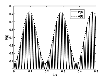
Figure 1: The time dependence of the neutrino oscillations probability in the twisting magnetic field in the case $\mu\gg\mu_{1,2}$ at small values of $\omega$.

As one can see on this figure, the rapidly varying transition probability $P(t)$ (solid line) is modulated by the slowly varying function $A(t)$ (dashed line). This time dependence is different from that described in Ref. twisting .

It is also possible to see on Fig. 1 that the typical time scale of the amplitude modulation of the transition probability is about $T_{A}\approx 0.1\thinspace\text{s}$. The production rate of right-handed neutrinos in the early Universe should be less than the expansion rate of the Universe in order not to affect the primordial nucleosynthesis prodrnuR . Hence one has $T_{A}h>1$, where

$$h\approx 1.24\times 10^{3}\left(\frac{T_{\mathrm{pl}}}{100\thinspace\text{MeV}}\right)^{2}\thinspace\text{s}^{-1},$$

is the Hubble parameter Wei72 and $T_{\mathrm{pl}}$ is the primordial plasma temperature. Supposing that neutrinos are at thermal equilibrium at $100\thinspace\text{MeV}$, i.e. $k\sim T_{\mathrm{pl}}$, we get that $T_{A}h\sim 100\gg 1$.

Despite the mentioned above discrepancy it is interesting to compare the result of this section [Eq. (54)] with the analogous transition probability formula for Majorana neutrinos twisting at small mixing angle $\theta\to 0$. Note that in this situation magnetic moments matrices in Eqs. (III) and (III) [or Eq. (26)] coincide. In this limit we obtain from Eq. (54) the following transition probability:

$$P_{\nu^{\mathrm{L}}_{\beta}\to\nu^{\mathrm{R}}_{\alpha}}(t)= \frac{(\mu B)^{2}}{\Omega_{M}^{2}}\sin^{2}(\Omega_{M}t),$$ (57)

where $\Omega_{M}=\sqrt{(\mu B)^{2}+[\Phi(k)+\omega/2]^{2}}$. It can be seen that Eq. (57) coincides with the transition probabilities derived in Ref. twisting where spin-flavor oscillations of Majorana neutrinos in twisting magnetic fields were studied on the basis of the quantum mechanical approach.

It should be also noticed that the transition probability in Eq. (54) vanishes at high frequencies, $\omega\gg\max(m_{a},\mu B)$, due to the dependence of the oscillations phase on $\omega$ [see Eq. (40)]. This phenomenon was also mentioned in our paper Dvo07YadFiz in which we examined spin-flavor oscillations of Majorana neutrinos in rapidly varying external fields.

IV Quantum mechanical description of neutrino oscillations in a twisting magnetic field

In this section we demonstrate that the analog of the main results, yielded in Secs. III.1 and III.2 within the Dirac-Pauli equation approach, can be also obtained with help of the standard quantum mechanical treatment of spin-flavor oscillations. The consistency between these two approaches is discussed.

To study neutrinos evolution in frames of the Schrödinger equation approach it is convenient to make the coordinates transformation. We assume that $\mathbf{k}=(0,0,k)$ and $\mathbf{B}=B(\sin\omega t,\cos\omega t,0)$. Now the Schrödinger equation and the effective Hamiltonian for the neutrinos mass eigenstates have the form,

$$\mathrm{i}\dot{\Psi}=H\Psi,\quad H=\begin{pmatrix}H_{\mathrm{mass}}&H_{B}\\ H_{B}^{\dagger}&H_{\mathrm{mass}}\ \end{pmatrix},$$ (58)

where $H_{\mathrm{mass}}=\mathrm{diag}(\mathcal{E}_{1},\mathcal{E}_{2})$, $\mathcal{E}_{1,2}=\sqrt{m_{1,2}^{2}+k^{2}}$ and

$$H_{B}=-(B_{x}+\mathrm{i}B_{y})\begin{pmatrix}\mu_{1}&\mu\\ \mu&\mu_{2}\ \end{pmatrix}=-\mathrm{i}(\mu_{ab})Be^{-\mathrm{i}\omega t},$$ (59)

where $\mu_{1,2}$ and $\mu$ are the elements of the magnetic moments matrix (26). The neutrinos wave function has the following form: $\Psi^{\mathrm{T}}=(\psi_{1}^{\mathrm{L}},\psi_{2}^{\mathrm{L}},\psi_{1}^{\mathrm{R}},\psi_{2}^{\mathrm{R}})$, where $\psi_{1,2}^{\mathrm{L,R}}$ are one-component functions. It can be seen that Eqs. (58) and (59) is the generalization, for the case of Dirac neutrinos, of the corresponding expressions used in Ref. twisting . The initial condition for the wave function $\Psi$ follows from Eq. (27),

$$\Psi^{\mathrm{T}}(0)=(\sin\theta,\cos\theta,0,0).$$ (60)

Let us make the matrix transformation,

$$\Psi= \mathfrak{V}\widetilde{\Psi},$$

$$\mathfrak{V}= \mathrm{diag}(e^{-\mathrm{i}\omega t/2},e^{-\mathrm{i}\omega t/2},e^{\mathrm{i}\omega t/2},e^{\mathrm{i}\omega t/2})$$ (61)

The Hamiltonian $\tilde{H}$ governing the time evolution of the modified wave function $\widetilde{\Psi}$ is presented in the form

$$\tilde{H}=\begin{pmatrix}H_{\mathrm{mass}}-\widehat{\mathds{1}}\omega/2&-\mathrm{i}(\mu_{ab})B\\ \mathrm{i}(\mu_{ab})B&H_{\mathrm{mass}}+\widehat{\mathds{1}}\omega/2\ \end{pmatrix},$$ (62)

where $\widehat{\mathds{1}}$ is the $2\times 2$ unit matrix. The initial condition for $\widetilde{\Psi}$ coincides with that for $\Psi$ [see Eq. (60)] due to the special form of the matrix $\mathfrak{V}$ in Eq. (IV).

Then we look for the solutions to the Schrödinger equation $\mathrm{i}\mathrm{d}\widetilde{\Psi}/\mathrm{d}t=\tilde{H}\widetilde{\Psi}$, with the Hamiltonian given in Eq. (62), in the form $\widetilde{\Psi}\sim e^{-\mathrm{i}\lambda t}$. The secular equation for $\lambda$ is the forth order algebraic equation in general case. However it can be solved in two situations.

IV.1 Diagonal magnetic moments matrix

In the case when $\mu=0$ and $\mu_{1,2}\neq 0$ the roots of the secular equation are

$$\lambda_{a}^{\pm{}}=\mathcal{E}_{a}\pm\mathcal{M}_{a},\quad a=1,2,$$ (63)

where $\mathcal{M}_{a}$ is defined in Eq. (III). The basis spinors $u_{a}^{\pm{}}$, which are the eigenvectors of the Hamiltonian $\tilde{H}$ are expresed in the following way:

$$u_{1}^{+{}}= \frac{1}{\sqrt{2\mathcal{M}_{1}}}\begin{pmatrix}-\mathrm{i}\mu_{1}B/\mathcal{Z}_{1}\\ 0\\ \mathcal{Z}_{1}\\ 0\ \end{pmatrix},$$

$$u_{1}^{-{}}= \frac{1}{\sqrt{2\mathcal{M}_{1}}}\begin{pmatrix}\mathcal{Z}_{1}\\ 0\\ -\mathrm{i}\mu_{1}B/\mathcal{Z}_{1}\\ 0\ \end{pmatrix},$$

$$u_{2}^{+{}}= \frac{1}{\sqrt{2\mathcal{M}_{2}}}\begin{pmatrix}0\\ -\mathrm{i}\mu_{2}B/\mathcal{Z}_{2}\\ 0\\ \mathcal{Z}_{2}\ \end{pmatrix},$$

$$u_{2}^{-{}}= \frac{1}{\sqrt{2\mathcal{M}_{2}}}\begin{pmatrix}0\\ \mathcal{Z}_{2}\\ 0\\ -\mathrm{i}\mu_{2}B/\mathcal{Z}_{2}\ \end{pmatrix},$$ (64)

where $\mathcal{Z}_{1,2}=\sqrt{\mathcal{M}_{1,2}+\omega/2}$. Note that the vectors $u_{a}^{\pm{}}$ correspond to the eigenvalues $\lambda_{a}^{\pm{}}$.

The general solution to the Schrödinger evolution equation has the form,

$$\widetilde{\Psi}(t)=\sum_{a=1,2}\sum_{\zeta=\pm 1}\alpha_{a}^{(\zeta)}u_{a}^{(\zeta)}\exp(-\mathrm{i}\lambda_{a}^{(\zeta)}t),$$ (65)

where the coefficients $\alpha_{a}^{(\zeta)}$ should be chosen so that to satisfy the initial condition in Eq. (60). We choose these quantities as

$$\alpha_{1}^{+{}}= \sin\theta\frac{1}{\sqrt{2M_{1}}}\frac{\mathrm{i}\mu_{1}B}{\mathcal{Z}_{1}},\quad\alpha_{1}^{-{}}=\sin\theta\frac{\mathcal{Z}_{1}}{\sqrt{2M_{1}}},$$

$$\alpha_{2}^{+{}}= \cos\theta\frac{1}{\sqrt{2M_{2}}}\frac{\mathrm{i}\mu_{2}B}{\mathcal{Z}_{2}},\quad\alpha_{2}^{-{}}=\sin\theta\frac{\mathcal{Z}_{1}}{\sqrt{2M_{1}}},$$ (66)

Then using Eqs. (IV) and (63)-(IV.1) we get the right-polarized components of the wave function $\Psi$ in the form

$$\psi_{1}^{\mathrm{R}}(t)= \exp[-\mathrm{i}(\mathcal{E}_{1}-\omega/2)t]\sin\theta\sin(\mathcal{M}_{1}t)\frac{\mu_{1}B}{\mathcal{M}_{1}},$$

$$\psi_{2}^{\mathrm{R}}(t)= \exp[-\mathrm{i}(\mathcal{E}_{2}-\omega/2)t]\cos\theta\sin(\mathcal{M}_{2}t)\frac{\mu_{2}B}{\mathcal{M}_{2}}.$$ (67)

Finally taking into account Eqs. (23), (24) and (IV.1) we arrive to the right-handed component of $\nu_{\alpha}$,

$$\nu_{\alpha}^{\mathrm{R}}(t)= \cos\theta\psi_{1}^{\mathrm{R}}(t)-\sin\theta\psi_{2}^{\mathrm{R}}(t)$$

$$= \sin\theta\cos\theta e^{\mathrm{i}\omega t/2}\bigg{[}\exp(-\mathrm{i}\mathcal{E}_{1}t)\sin(\mathcal{M}_{1}t)\frac{\mu_{1}B}{\mathcal{M}_{1}}$$

$$-\exp(-\mathrm{i}\mathcal{E}_{2}t)\sin(\mathcal{M}_{2}t)\frac{\mu_{2}B}{\mathcal{M}_{2}}\bigg{]}.$$ (68)

One can see from Eq. (IV.1) that the expression for $\nu_{\alpha}^{\mathrm{R}}$ obtained in frames of the Schrödinger approach coincides (to within some irrelevant phase factor) with the analogous expression derived using the Dirac-Pauli equation [see Eq. (38)].

IV.2 Non-diagonal magnetic moments matrix

In the situation when $\mu_{1,2}=0$ and $\mu\neq 0$ the secular equation can be also solved analytically and the corresponding roots are

$$\lambda_{1,2}^{+{}}=\bar{\mathcal{E}}\pm\Omega_{+{}},\quad\lambda_{1,2}^{-{}}=\bar{\mathcal{E}}\pm\Omega_{-{}},$$ (69)

where $\bar{\mathcal{E}}=(\mathcal{E}_{1}+\mathcal{E}_{2})/2$ and $\Omega_{\pm{}}$ are given in Eq. (52). The eigenvectors of the Hamiltonian $\tilde{H}$ have the following form:

$$u_{1,2}= \frac{1}{\sqrt{2\Omega_{+{}}}}\begin{pmatrix}0\\ \mp\mathrm{i}\mu B/R_{\pm{}}\\ R_{\pm{}}\\ 0\ \end{pmatrix},$$

$$v_{1,2}= \frac{1}{\sqrt{2\Omega_{-{}}}}\begin{pmatrix}\mp\mathrm{i}\mu B/S_{\mp{}}\\ 0\\ 0\\ S_{\mp{}}\ \end{pmatrix},$$ (70)

where $R_{\pm{}}=\sqrt{\Omega_{+{}}\pm\omega_{+{}}/2}$, $S_{\pm{}}=\sqrt{\Omega_{-{}}\pm\omega_{-{}}/2}$ and $\omega_{\pm{}}$ are given in Eq. (52). The spinors $u_{1,2}$ and $v_{1,2}$ in Eq. (IV.2) correspond to the eigenvalues $\lambda_{1,2}^{+{}}$ and $\lambda_{1,2}^{-{}}$ respectively.

The general solution to the Schrödinger equation for the function $\widetilde{\Psi}$ takes the form,

$$\widetilde{\Psi}(t)= \exp(-\mathrm{i}\bar{\mathcal{E}}t)[\alpha_{1}u_{1}\exp(-\mathrm{i}\Omega_{+{}}t)+\alpha_{2}u_{2}\exp(\mathrm{i}\Omega_{+{}}t)$$

$$+\beta_{1}v_{1}\exp(-\mathrm{i}\Omega_{-{}}t)+\beta_{2}v_{2}\exp(\mathrm{i}\Omega_{-{}}t)],$$ (71)

We again choose the coefficients $\alpha_{1,2}$ and $\beta_{1,2}$ in Eq. (IV.2) to satisfy the initial condition in Eq. (60). These coefficients have to be chosen as

$$\alpha_{1,2}=\pm\mathrm{i}\cos\theta\frac{R_{\mp{}}}{\sqrt{2\Omega_{+{}}}},\quad\beta_{1,2}=\pm\mathrm{i}\sin\theta\frac{S_{\pm{}}}{\sqrt{2\Omega_{-{}}}},$$ (72)

With help of Eqs. (IV) and (69)-(72) we obtain the right-handed components of the wave function $\Psi$ in the form

$$\psi_{1}^{\mathrm{R}}(t)= \mu B\cos\theta\exp[-\mathrm{i}(\bar{\mathcal{E}}-\omega/2)t]\frac{\sin(\Omega_{+{}}t)}{\Omega_{+{}}},$$

$$\psi_{2}^{\mathrm{R}}(t)= \mu B\sin\theta\exp[-\mathrm{i}(\bar{\mathcal{E}}-\omega/2)t]\frac{\sin(\Omega_{-{}}t)}{\Omega_{-{}}}.$$ (73)

On the basis of Eq. (IV.2) we receive the wave function $\nu_{\alpha}^{\mathrm{R}}$ as

$$\nu_{\alpha}^{\mathrm{R}}(t)= \mu B\exp[-\mathrm{i}(\bar{\mathcal{E}}-\omega/2)t]$$

$$\times\left(\cos^{2}\theta\frac{\sin\Omega_{+{}}t}{\Omega_{+{}}}-\sin^{2}\theta\frac{\sin\Omega_{-{}}t}{\Omega_{-{}}}\right).$$ (74)

Comparing Eq. (IV.2) with the analogous expression (53) derived in frames of the Dirac-Pauli equation approach we again find an agreement to within the phase factor.

It should be however mentioned that using the quantum mechanical treatment of spin-flavor oscillations one cannot reproduce the expression for the phase of the neutrino oscillations (40). It means that in Eqs. (IV.1) and (IV.2) we have the standard quantum mechanical vacuum oscillations phase $\Phi_{QM}(k)=\delta m^{2}/(4k)$.

V Applications

Let us discuss the applicability of our results to one specific oscillation channel, $\nu_{\mu}^{\mathrm{L}}\xleftrightarrow{B}\nu_{\tau}^{\mathrm{R}}$. According to the recent neutrino oscillations data (see, e.g., Ref. MalSchTorVal04 ) the mixing angle between $\nu_{\mu}$ and $\nu_{\tau}$ is close to its maximal value of $\pi/4$. For such a mixing angle the magnetic moment matrix given in Eq. (26) is expressed in the form,

$$({\mu}_{ab})\approx\\ \begin{pmatrix}[{M}_{\tau\tau}+{M}_{\mu\mu}]/2+{M}_{\tau\mu}&-[{M}_{\tau\tau}-{M}_{\mu\mu}]/2\\ -[{M}_{\tau\tau}-{M}_{\mu\mu}]/2&[{M}_{\tau\tau}+{M}_{\mu\mu}]/2-{M}_{\tau\mu}\ \end{pmatrix}.$$ (75)

Eq. (39) is valid when this matrix is close to diagonal, i.e. if $|({M}_{\tau\tau}-{M}_{\mu\mu})/2|\ll|({M}_{\tau\tau}+{M}_{\mu\mu})/2\pm{M}_{\tau\mu}|$. In contrast to the mixing angles, experimental data and theoretical predictions for the values of neutrino magnetic moments are not very reliable magnmomDM . However it is known that the diagonal magnetic moments $M_{\lambda\lambda}$ could be very small in the extensions of the standard model ${M}_{\lambda\lambda}\sim 10^{-19}({m}_{\lambda\lambda}/\text{eV})\mu_{\mathrm{B}}$ nuMM . The transition magnetic moments, ${M}_{\tau\mu}$ in our notations, can be much greater up to the experimental limit of $10^{-10}\mu_{\mathrm{B}}$ Yao06 . One can see that for any conceivable values of the masses of the known neutrinos, ${M}_{\mu\mu}$ and ${M}_{\tau\tau}$ are several orders of magnitude smaller than $10^{-10}\mu_{\mathrm{B}}$. Our result (39) is valid in this case.

It is worth mentioning that Eqs. (33) and (42) are in principle applicable for particles with arbitrary initial conditions, e.g., with small initial momenta. Therefore one can discuss the evolution and oscillations of relic neutrinos. These particles can gravitationally cluster in the Galaxy RinWon05 . It is possible to relate the temperatures of relic neutrinos and CMB protons, $T_{\nu}$ and $T_{\gamma}$ respectively,

$$T_{\nu}=\left(\frac{4}{11}\right)^{1/3}T_{\gamma}\approx 0.72T_{\gamma}.$$ (76)

For the present value $T_{\gamma}=2.7^{\circ}\thinspace\mathrm{K}$ we get $T_{\nu}\approx 1.93^{\circ}\thinspace\mathrm{K}$ RinWon05 . Using the estimate for the neutrino mass $m\sim 0.1\thinspace\mathrm{eV}$, because the sum of all neutrinos masses should be less than $1\thinspace\mathrm{eV}$ HanRaf06 , and taking into account that these neutrinos are non-relativistic particles, one obtains the typical momentum of a relic neutrino $k\sim 7\times 10^{-3}\thinspace\mathrm{eV}$. For example, to realize the ”non-standard” neutrino propagation regime described in item 1 of Sec. II one should use an undulator with the frequency $|\omega|\sim 2k$ or with the period $L=2\pi/\omega\sim 0.1\thinspace\mathrm{mm}$.

Strong periodic electromagnetic fields, with a short spatial oscillations length, can be found in crystals Ugg05 . In Ref. Bel03 it was proposed to manufacture deformed crystals with submillimeter periods. The undulator radiation was recently reported in Ref. Bar05 to be produced in undulators with periods of $0.1-1\thinspace\mathrm{mm}$. Therefore artificial crystalline undulators with required periods are used in various experiments and hence they can serve as a good tool to explore properties of relic neutrinos. It should be mentioned that neutrino scattering on a polarized target and possible tests of neutrino magnetic moment were examined in Ref. RasSem00 .

VI Summary

We have described the evolution of Dirac neutrinos in matter and in a twisting magnetic field. We have applied the recently developed approach (see Refs. FOvac ; Dvo06EPJC ; DvoMaa07 ) which is based on the exact solutions to the Dirac equation in an external field with the given initial condition.

First (Sec. II) we have found the solution to the Dirac equation for a neutral $1/2$-spin particle weakly interacting with background matter, that is equivalent to an external axial-vector field, and non-minimally coupled to an external electromagnetic field due to the possible presence of an anomalous magnetic moment. We have discussed the situation when a neutrino interacts with the twisting magnetic field. The energy spectrum and basis spinors have been obtained. We have applied these results to derive the transition probability of spin oscillations in matter under the influence of the twisting magnetic field. The scope of the standard quantum mechanical approach to the description of neutrino spin oscillations has been analyzed.

Then (Sec. III) we have used the obtained solution to the Dirac equation for the description of neutrino spin-flavor oscillations in a twisting magnetic field. We supposed that two Dirac neutrinos could mix and have non-vanishing matrix of magnetic moments. Moreover the mass and magnetic moments matrices in the flavor eigenstates basis are generally independent, i.e. the diagonalization of the mass matrix, that means the transition to the mass eigenstates basis, does not lead to the diagonalization of the magnetic moments matrix. We have discussed two possibilities.

In Sec. III.1 we have assumed that magnetic moments matrix in the mass eigenstates basis has great diagonal elements compared to the non-diagonal ones. In this case one can analyze neutrino spin-flavor oscillations perturbatively. Note that the perturbative approach allows one to discuss neutrinos with an arbitrary initial condition. For instance, the evolution of particles with small initial momenta can be accounted for. The appearance of non-perturbative phenomena like resonances is analyzed with an example of active-to-sterile neutrinos oscillations. We have discussed the opposite situation in Sec. III.2, i.e. the magnetic moment matrix with the great non-diagonal elements. In this case one had to treat the evolution of the system non-perturbatively. We have demonstrated that this situation is analogous to beatings resulting from the superposition of two oscillations. In both cases we have obtained neutrino wave functions, consistent with the initial conditions, and the transition probabilities. Note that all the results are in agreement with our previous work DvoMaa07 if we set $\omega=0$, i.e. discuss a constant transversal magnetic field. We have also examined some limiting cases and compared our results with the previous studies.

It has been shown in Sec. IV that one can derive the analog of the major results obtained in Secs. III.1 and III.2 using the Schrödinger evolution equation approach for the description of spin-flavor oscillations of Dirac neutrinos. The correspondence between these two approaches has been considered.

In Sec. V we have discussed magnetic moments matrices in various theoretical models which predict neutrinos magnetic moments. The validity of our approach for these situations has been considered. The applications of our results to the studying of cosmological neutrinos in laboratory conditions have been examined. In particular we have suggested that artificial crystalline undulators could be useful for such a research.

The results obtained in the present work are valid for arbitrary magnetic field strength. The general case of spin-flavor oscillations of Dirac neutrinos in a twisting magnetic field with an arbitrary magnetic moment matrix has not been studied analytically earlier. Both experimental and theoretical information about magnetic moments of Dirac neutrinos is known to be very limited (see, e.g. Refs. magnmomDM ; Yao06 ). Therefore our results can be helpful since they enable one to describe phenomenologically spin-flavor oscillations of Dirac neutrinos under the influence of the magnetic field in question provided neutrinos possess non-vanishing matrix of magnetic moments. Although we consider neutrinos, it is possible to straightforwardly apply our formalism to the description of any $1/2$-spin particles.

References

• (1) J. Schechter and J. W. F. Valle, Phys. Rev. D 24, 1883 (1981); M. B. Voloshin, M. I. Vysotskiĭ, and L. B. Okun’, JETP 64, 446 (1986); Sov. J. Nucl. Phys. 44, 440 (1986); E. Akhmedov, Phys. Lett. B 213, 64 (1988); C.-S. Lim and W. J. Marciano, Phys. Rev. D 37, 1368 (1988).
• (2) B. C. Chauhan, J. Pulido and R. S. Raghavan, JHEP 0507, 051 (2005), hep-ph/0504069; J. Barranco et al., Phys. Rev. D 66, 093009 (2002), hep-ph/0207326.
• (3) A. B. Balantekin and P. Loreti, Phys. Rev. D 48, 5496 (1993); A. Friedland and A. Gruzinov, Astropart. Phys. 19, 575 (2003), hep-ph/0202095.
• (4) M. Picariello et al., to be published in JHEP, 0705.4070 [hep-ph].
• (5) E. Kh. Akhmedov and J. Pulido, Phys. Lett. B 553, 7 (2003), hep-ph/0209192; A. B. Balantekin and C. Volpe, Phys. Rev. D 72, 033008 (2005), hep-ph/0411148.
• (6) H. V. Klapdor-Kleingrothaus, et al., Phys. Lett. B 586, 198 (2004), hep-ph/0404088.
• (7) S. R. Elliott and J. Engel, J. Phys. G 30, R183 (2004), hep-ph/0405078.
• (8) V. B. Semikoz, Nucl. Phys. B 498, 39 (1997), hep-ph/9611383.
• (9) M. Dvornikov, Phys. Lett. B 610, 262 (2005), hep-ph/0411101; in Proceedings of the IPM school and conference on Lepton and Hadron Physics, Tehran, 2006, ed. by Y. Farzan, eConf C0605151 (2007), hep-ph/0609139; hep-ph/0610047.
• (10) M. Dvornikov, Eur. Phys. J. C 47, 437 (2006), hep-ph/0601156; to be published in J. Phys. Conf. Ser., 0708.2975 [hep-ph].
• (11) M. Dvornikov and J. Maalampi, Phys. Lett. B 657, 217 (2007), hep-ph/0701209; M. Dvornikov, to be published in proceedings of the $14^{\mathrm{th}}$ International Baksan School ”Particles and Cosmology”, 0708.3572 [hep-ph].
• (12) M. S. Dvornikov and A. I. Studenikin, Phys. At. Nucl. 64, 1624 (2001); ibid. 67, 719 (2004); E. Kh. Akhmedov and M. Yu. Khlopov, Sov. J. Nucl. Phys. 47, 689 (1988); A. Egorov, A. Lobanov, and A. Studenikin, Phys. Lett. B 491, 137 (2000), hep-ph/9910476.
• (13) M. Dvornikov, Phys. At. Nucl. 70, 342 (2007), hep-ph/0410152.
• (14) A. Yu. Smirnov, Phys. Lett. B 260, 161 (1991); E. Kh. Akhmedov, P. I. Krastev, and A. Yu. Smirnov, Z. Phys. C 48, 701 (1991); E. Kh. Akhmedov, S. T. Petcov, and A. Yu. Smirnov, Phys. Rev. D 48, 2167 (1993), hep-ph/9301211.
• (15) M. Dvornikov and A. Studenikin, JHEP 09, 016 (2002), hep-ph/0202113.
• (16) E. Elizalde, E. J. Ferrer and V. de la Incera, Phys. Rev. D 70, 043012 (2004), hep-ph/0404234.
• (17) A. Studenikin and A. Ternov, Phys. Lett. B 608, 107 (2005), hep-ph/0412408; A. E. Lobanov, Phys. Lett. B 608, 136 (2005), hep-ph/0506007.
• (18) P. Keränen et al., Phys. Lett. B 597, 374 (2004), hep-ph/0401082.
• (19) M. Maltoni et al., New J. Phys. 6, 122 (2004), hep-ph/0405172.
• (20) H. Athar, Phys. Lett. B 366, 229 (1996).
• (21) A. D. Dolgov, Phys. Rept. 370, 333 (2002), hep-ph/0202122; M. Dvornikov, Int. J. Mod. Phys. A 21, 2403 (2006), hep-ph/0501063.
• (22) S. Weinberg, Gravitation and Cosmology: Principles and Applications of the General Theory of Relativity (Wiley, New York, 1972), p. 534.
• (23) N. F. Bell et al., Phys. Rev. Lett. 95, 151802 (2005), hep-ph/0504134; N. F. Bell et al., Phys. Lett. B 642, 377 (2006), hep-ph/0606248.
• (24) K. Fujikawa and R. E. Shrock, Phys. Rev. Lett. 45, 963 (1980); M. Dvornikov and A. Studenikin, Phys. Rev. D 69, 073001 (2004), hep-ph/0305206.
• (25) W.-M. Yao et al., J. Phys. G 33, 1 (2006).
• (26) A. Ringwald and Y. Wong, JCAP 0506, 013 (2005), hep-ph/0410136.
• (27) S. Hannestad and G. G. Raffelt, JCAP 0611, 016 (2006), astro-ph/0607101.
• (28) U. I. Uggerhøj, Rev. Mod. Phys. 77, 1131 (2005).
• (29) S. Bellucci et al., Phys. Rev. Lett. 90, 034801 (2003), physics/0208028.
• (30) V. T. Baranov et al., JETP Lett. 82, 562 (2005).
• (31) T. I. Rashba and V. B. Semikoz, Phys. Lett. B 479, 218 (2000), hep-ph/0003099.