Abstract

We present the estimate of the branching ratio for the rare decay $\bar{B}^{0}\rightarrow D^{*}\gamma$. We use QCD factorization approach in order to compute the amplitude of the process. The calculation is carried out with the leading order accuracy. The appearing non-perturbative matrix elements have been estimated using the large$-N_{c}$ limit and QCD sum rule approach. We obtained that $\mathcal{B}(\bar{B}^{0}\rightarrow D^{*}\gamma)\simeq 1.52\times 10^{-7}$. Such value of the branching fraction is too small in order to be measured at present experiments.

1 Introduction

The different decay processes mediated by $b\rightarrow cd\bar{u}$ quark decay attract a lot of attention of both experimentalist and theoreticians. Corresponding hadron decays include various processes like $\bar{B}\rightarrow D+(\pi,\rho,K,...)$. There are a lot of experimental results for the different decay modes, see for instance [2] and the references there. From the theoretical side the progress in the phenomenological description of the data can be related with the factorization approach developed last years. The factorization theorems for the different decay channels have been discussed in literature [3, 4, 5, 6, 7, 8]. In the present paper we would like to consider one particular decay mode $B\rightarrow D^{*}+\gamma$ which remained beyond the considerations mentioned above.

From the experimental point of view the process can be clearly observed due to the higher energy of the outgoing photon ($E_{\gamma}\simeq 2.3$GeV). The search of this rare decay have already been made by CLEO [9] and BABAR [10] collaborations. Despite the process has not been observed ($\mathcal{B}(\bar{B}^{0}\rightarrow D^{*}\gamma)<2.5\times 10^{-5}$ [10]) the increasing statistics of the $B-$factories may provide new opportunities for the better analysis. The various existing theoretical models [11, 12, 13] estimate the branching to be of order of $10^{-6}$. Potentially, such cross section can be observed despite to the small value and therefore the more qualitative theoretical analysis is desirable.

In present paper we use the factorization technique developed last years for the heavy quarks decays in order to derive the leading order factorization formula for the amplitude of the process and estimate the branching ratio. Our presentation is organized as follows. Sec. 2 contains the necessary definitions and derivation of the leading order factorization calculations. In Sec.3 we consider the arising soft matrix elements and construct the models for these non-perturbative functions using large$-N_{c}$ limit and QCD sum rules. This section contains also our main results, the summary and discussions.

2 The leading order amplitude

The decay amplitude $\bar{B}^{0}(P_{B})\rightarrow D^{*}(P_{D})\gamma(q)$ is given by the matrix element

$$A_{D^{\ast}\gamma} = ~{}\sqrt{4\pi\alpha}~{}i\int dxe^{i(qx)}~{}\varepsilon_{\gamma}^{*\mu}\left\langle P_{D},\varepsilon^{*}_{D}\left|T\left\{J_{\mu}^{em}(x),H_{eff}(0)\right\}\right|P_{B}\right\rangle$$ (1)

$$= \frac{1}{2(q\cdot P_{D})}i\varepsilon^{\mu\nu\sigma\rho}(\varepsilon^{*}_{\gamma})_{\mu}(\varepsilon^{*}_{D})_{\nu}q_{\sigma}(P_{D})_{\rho}\,F_{1}+\left\{\left(\varepsilon^{*}_{\gamma}\cdot\varepsilon^{*}_{D}\right)-\frac{1}{(q\cdot P_{D})}(q\cdot\varepsilon^{*}_{D})(P_{D}\cdot\varepsilon^{*}_{\gamma})\right\}\,F_{2}$$ (2)

which is described by the two form factors $F_{1,2}$. Here we accept standard notation $\alpha=\frac{e^{2}}{4\pi}\simeq 1/137$ and $\varepsilon^{*}_{\gamma,D}$ denotes photon and $D-$meson polarization vector respectively. The kinematics of the decay is very simple. As usual, we choose the frame where $B-$meson is at rest. Then the the components of the momenta read

$$P_{B} = P_{D}+q,\,\,P^{2}_{B}=M^{2}_{B},\,\,P^{2}_{D}=M^{2}_{D},\,\,q^{2}=0,$$ (3)

$$P_{B} = M_{B}v,\,\,P_{D}=M_{D}v^{\prime},\,\,q=2E_{\gamma}\frac{n}{2},$$ (4)

$$v = (1,0,0,0)=\frac{\bar{n}}{2}+\frac{n}{2},\,\,n^{2}=\bar{n}^{2}=0,\,\,n\cdot\bar{n}=2,$$ (5)

$$v^{\prime} = \left(\frac{M_{B}^{2}+M_{D}^{2}}{2M_{B}M_{D}},0,0,\frac{M_{B}^{2}-M_{D}^{2}}{2M_{B}M_{D}}\right)=\frac{1}{x}\frac{\bar{n}}{2}+x\frac{n}{2},\,\,x=M_{D}/M_{B},$$ (6)

$$E_{\gamma} = \frac{M_{B}^{2}-M_{D}^{2}}{2M_{B}},$$ (7)

where we introduced the light-cone vectors $n,\bar{n}$ and for arbitrary vector $a$ one has

$$a=a_{+}\frac{\bar{n}}{2}+a_{-}\frac{n}{2}+a_{\bot}$$ (8)

Substituting the numerical values of the heavy meson masses $M_{D}=2$GeV and $M_{B}=5.28$GeV one finds $E_{\gamma}\approx 2.3$GeV, i.e. the photon energy is quite large. The width is given by

$$\Gamma_{D^{\ast}\gamma}=\frac{1}{32\pi}\frac{M_{B}^{2}-M_{D}^{2}}{M_{B}^{3}}\left(~{}\left|F_{1}\right|^{2}+4\left|F_{2}\right|^{2}\right)$$ (9)

Using the experimental constrain for the branching [10]

$$\mathcal{B}(\bar{B}^{0}\rightarrow D^{\ast 0}\gamma)<2.5\times 10^{-5}$$ (10)

and the lifetime $\tau_{B^{0}}=1.536\times 10^{-12}~{}s$ one can find for the combination of the form factors in (9)

$$\left|F_{1}\right|^{2}+4\left|F_{2}\right|^{2}<1.1\times 10^{-3}\left(G_{F}\sqrt{2\pi\alpha}\right)^{2},$$ (11)

where the coefficient $G_{F}\sqrt{2\pi\alpha}$ is introduced for convenience.

Our task is to compute the form factors $F_{1,2}$ in the limit $m_{b},m_{c}\rightarrow\infty$ with $m_{c}/m_{b}$ fixed. The effective Hamiltonian in the matrix element (1) reads

$$H_{eff} = \frac{G_{F}}{\sqrt{2}}V_{cb}V_{ud}^{\ast}\left[C_{1}~{}(\bar{c}b)_{V-A}(\bar{d}u)_{V-A}+C_{2}~{}\left(\bar{d}b\right)_{V-A}\left(\bar{c}u\right)_{V-A}\right]$$ (12)

where as usually $V-A=\gamma_{\mu}(1-\gamma_{5})$ and the color indices are not shown explicitly. Let us introduce the following parametrization for the amplitude (1):

$$A_{D^{\ast}\gamma}=\sqrt{M_{D}M_{B}}\sqrt{2\pi\alpha}\,\,G_{F}~{}V_{cb}V_{ud}^{\ast}~{}\left[~{}\alpha^{\text{f}}+~{}\alpha^{\text{nf}}\right],$$ (13)

where the coefficients $\alpha^{\text{nf}}$ and $\alpha^{\text{f}}$ are related to the matrix elements of the two operators in the (12):

$$\alpha^{\text{f}} \displaystyle=i\int dx~{}e^{i(qx)}~{}\varepsilon_{\gamma}^{*\mu}\left\langle v^{\prime}\left|T\left\{J^{em}_{\mu}(x),C_{2}\left(\bar{d}b\right)_{V-A}\left(\bar{c}u\right)_{V-A}\right\}\right|v\right\rangle,$$ (14)

$$\alpha^{\text{nf}} \displaystyle=i\int dx~{}e^{i(qx)}~{}\varepsilon_{\gamma}^{*\mu}\left\langle v^{\prime}\left|T\left\{J^{em}_{\mu}(x),C_{1}(\bar{c}b)_{V-A}(\bar{d}u)_{V-A}\right\}\right|v\right\rangle,$$ (15)

The meaning of the superscripts ”f, nf” will be explained below. In these formulas we assume that the meson states $|v\rangle$, $\langle v^{\prime}|$ have mass independent HQET normalization.

In the large mass limit the energy of the photon is also large $E_{\gamma}\sim m_{Q}\rightarrow\infty$. The emission of such higher energy photon is related with short distance subprocess. In some sense, the similar situation is encountered in the case of semi-leptonic decay $B\rightarrow\gamma l\nu$. The difference with respect to our case is in the more complicate structure of the matrix element (1). Consider the simplest diagrams which can contribute at the leading order Fig.1.

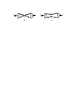
Figure 1: The leading order diagrams $a,\,b$ denote the graphs for the form factors $\alpha^{\text{f}}$

and $\alpha^{\text{nf}}$ respectively. The crossed lines denotes the emission of the photon.

The analytical expression for the case $\alpha^{\text{f}}$ reads

$$\alpha^{\text{f}}=4iC_{2}\int dx\,e^{i(qx)}\left\langle v^{\prime}\left|e_{d}~{}\bar{c}~{}\gamma^{\mu}P_{L}~{}u~{}\bar{d}(x)~{}\hat{\varepsilon}^{*}_{\gamma}\hat{\Delta}(x,0)\gamma_{\mu}P_{L}~{}b(0)+e_{u}~{}\bar{d}(0)\gamma^{\mu}P_{L}b~{}\bar{c}(0)\gamma_{\mu}P_{L}~{}\hat{\Delta}(0,x)\hat{\varepsilon}^{*}_{\gamma}u(x)\right|v\right\rangle,$$ (16)

where $\Delta(x,y)$ is the fermion propagator in position space, $e_{u,d}$ are quark charges, and the hat denotes the contractions with the Dirac matrices $a_{\mu}\gamma^{\mu}=\hat{a}$ and $P_{L}=\frac{1}{2}(1-\gamma_{5})$. In the heavy quark limit one performs transition from the QCD heavy quark fields to the HQET fields:

$$b(0)\simeq H_{v},~{}\ \bar{c}(0)\simeq\bar{h}_{v^{\prime}}$$ (17)

Hence

$$\alpha^{\text{f}}\simeq 4C_{2}i\int dx~{}e^{i(qx)}\left\langle v^{\prime}\left|e_{d}~{}\bar{h}_{v^{\prime}}~{}\gamma^{\mu}P_{L}~{}u~{}\bar{d}(x)~{}\hat{\varepsilon}^{*}_{\gamma}\hat{\Delta}(x,0)\gamma^{\mu}P_{L}~{}H_{v}+e_{u}~{}\bar{d}~{}\gamma^{\mu}P_{L}H_{v}~{}\bar{h}_{v^{\prime}}~{}\Gamma~{}\hat{\Delta}(0,x)\hat{\varepsilon}^{*}_{\gamma}u(x)\right|v\right\rangle$$ (18)

$$=4iC_{2}\int dk\ e_{d}\left[~{}\hat{\varepsilon}^{*}_{\gamma}\hat{\Delta}(-k+q)\gamma^{\mu}P_{L}\right]_{\alpha\beta}~{}\int dx~{}e^{i(kx)}\left\langle v^{\prime}\left|\bar{h}_{v^{\prime}}\gamma_{\mu}P_{L}u~{}\left[\bar{d}_{\alpha}(x)~{}(H_{v})_{\beta}\right]\right|v\right\rangle+$$

$$4iC_{2}\int dl\ e_{u}\left[\gamma^{\mu}P_{L}~{}\hat{\Delta}(-l-q)\hat{\varepsilon}^{*}_{\gamma}\right]_{\alpha\beta}~{}\int dx~{}e^{-i(lx)}\left\langle v^{\prime}\left|\left[(\bar{h}_{v^{\prime}})_{\alpha}~{}u_{\beta}(x)\right]\bar{d}\gamma_{\mu}P_{L}H_{v}\right|v\right\rangle\,.$$ (19)

In the second line we performed the transition to the momentum space, indices $\alpha,\beta$ denote the spinor indices, $dk\equiv d^{4}k/(2\pi)^{4}$. To proceed further we assume that given expression is dominated by the region, where the momenta $k$ and $l$ are soft:

$$k_{i}\sim l_{i}\sim\bar{\Lambda},\,\,k^{2}\sim l^{2}\sim\bar{\Lambda}^{2},$$ (20)

where $\bar{\Lambda}\simeq M_{Q}-m_{Q}$ is the soft scale. Then in that region the expressions for the matrix elements $\langle v^{\prime}|...|v\rangle$ in (19) are defined only in terms of the long wave fields and can be understood as soft matrix elements. The expressions in the $[...]_{\alpha\beta}$ can be simplified for the large energy ($E_{\gamma}\sim m_{Q}$):

$$\hat{\varepsilon}^{*}_{\gamma}\hat{\Delta}(-k+q)\gamma^{\mu}P_{L} =\hat{\varepsilon}^{*}_{\gamma}\frac{i(-\hat{k}+\hat{q})}{(-k+q)^{2}+i\varepsilon}\gamma^{\mu}P_{L}\simeq\hat{\varepsilon}^{*}_{\gamma}\hat{q}\gamma^{\mu}P_{L}\frac{i}{\left[-2(kq)+i\varepsilon\right]},$$ (21)

$$\gamma^{\mu}P_{L}~{}\hat{\Delta}(-l-q)\hat{\varepsilon}^{*}_{\gamma} =\gamma^{\mu}P_{L}~{}\frac{i(-\hat{l}-\hat{q})}{(-l-q)^{2}+i\varepsilon}\hat{\varepsilon}^{*}_{\gamma}\simeq\gamma^{\mu}P_{L}~{}\hat{q}\hat{\varepsilon}^{*}_{\gamma}\frac{-i}{\left[2(lq)+i\varepsilon\right]}$$ (22)

Substituting these expressions into (19)

$$\alpha^{\text{f}} =4iC_{2}\int dk\ \frac{ie_{d}\left[\hat{\varepsilon}^{*}_{\gamma}\hat{q}\gamma^{\mu}P_{L}\right]_{\alpha\beta}}{\left[-2(kq)+i\varepsilon\right]}~{}\int dx~{}e^{i(kx)}\left\langle v^{\prime}\left|\bar{h}\gamma_{\mu}P_{L}u~{}\left[\bar{d}_{\alpha}(x)~{}H_{\beta}\right]\right|v\right\rangle$$

$$+4iC_{2}\int dl\ \frac{-ie_{u}\left[\gamma^{\mu}P_{L}~{}\hat{q}~{}\hat{\varepsilon}^{*}_{\gamma}\right]_{\alpha\beta}}{\left[2(lq)+i\varepsilon\right]}~{}\int dx~{}e^{-i(lx)}\left\langle v^{\prime}\left|\left[\bar{h}_{\alpha}~{}u_{\beta}(x)\right]~{}\bar{d}\gamma_{\mu}P_{L}H~{}\right|v\right\rangle$$ (23)

Performing integrations over $dk_{-}$ and $dk_{\bot}$ and then over the conjugate variables $x_{+}$ and $x_{\bot}$ (and similar for the second term with momentum $l$) we obtain

$$\alpha^{\text{f}} \displaystyle=C_{2}\frac{1}{2}\int dk_{+}\frac{-e_{d}\mbox{\rm tr}\{\hat{\varepsilon}^{*}_{\gamma}\hat{q}\gamma^{\mu}\gamma^{\rho}P_{R}\}}{\left[-2E_{\gamma}~{}k_{+}+i\varepsilon\right]}\int\frac{d\lambda_{1}}{2\pi}~{}e^{ik_{+}\lambda_{1}}\left\langle v^{\prime}\left|\bar{h}\gamma_{\mu}P_{L}u~{}\bar{d}\left(\lambda_{1}~{}n\right)\gamma_{\rho}P_{L}~{}H\right|v\right\rangle$$ (24)

$$\displaystyle+C_{2}\frac{1}{2}\int dl_{+}\ \frac{e_{u}\mbox{\rm tr}\{\gamma^{\mu}\hat{q}~{}\hat{\varepsilon}^{*}_{\gamma}\gamma^{\rho}P_{R}\}}{\left[2E_{\gamma}~{}l_{+}+i\varepsilon\right]}\int\frac{d\lambda_{2}}{2\pi}~{}e^{-il_{+}\lambda_{2}}\left\langle v^{\prime}\left|~{}\bar{h}~{}\gamma_{\rho}P_{L}u\left(\lambda_{2}~{}n\right)~{}\bar{d}\gamma_{\mu}P_{L}H\right|v\right\rangle.$$

The formula (24) represents the form factor $\alpha^{\text{f}}$ as a convolution of the soft light-cone matrix elements with the expression which, obviously, is associated with the hard coefficient function. The arguments of the fields which are not written explicitly in the eq.(24) are set to zero. From the structures of the traces one observes that only the combinations antisymmetrical with respect to exchange $\mu\leftrightarrow\rho$ survive in the soft matrix elements. Therefore we define

$$S_{d}^{[\sigma\rho]}(k_{+})=\text{AS}\int\frac{d\lambda_{1}}{2\pi}~{}e^{ik_{+}\lambda_{1}}\left\langle v^{\prime}\left|\bar{h}_{v^{\prime}}\gamma_{\sigma}P_{L}u~{}\bar{d}\left(\lambda_{1}~{}n\right)\gamma_{\rho}P_{L}~{}H_{v}\right|v\right\rangle,$$ (25)

$$S_{u}^{[\sigma\rho]}(l_{+})=\text{AS}\int\frac{d\lambda_{2}}{2\pi}~{}e^{-il_{+}\lambda_{2}}\left\langle v^{\prime}\left|~{}\bar{h}_{v^{\prime}}~{}\gamma_{\rho}P_{L}u\left(\lambda_{2}~{}n\right)~{}\bar{d}\gamma_{\sigma}P_{L}H_{v}\right|v\right\rangle,$$ (26)

where symbol ”AS” denotes antisymmetrisation with respect to indices $\left\{\sigma,\rho\right\}$, for instance

$$\text{AS}~{}\bar{n}^{\sigma}\varepsilon_{D}^{*\rho}=\frac{1}{2}\left(\bar{n}^{\sigma}\varepsilon_{D}^{*\rho}-\bar{n}^{\rho}\varepsilon_{D}^{*\sigma}\right)$$ (27)

The parametrisation of these functions can be written as

$$S_{u}^{[\sigma\rho]}(l_{+}) =\frac{i}{2}U^{\text{f}}(l_{+})~{}\text{AS}~{}\bar{n}_{\sigma}\left\{(\varepsilon^{*}_{D})_{\rho}-i\varepsilon_{{\bot}\rho\mu}\varepsilon_{D}^{*\mu}\right\}+\frac{i}{2}\tilde{U}^{\text{f}}(l_{+})~{}\text{AS}~{}\bar{n}_{\sigma}\left\{(\varepsilon^{*}_{D})_{\rho}+i\varepsilon_{{\bot}\rho\mu}\varepsilon_{D}^{*\mu}\right\},$$ (28)

$$S_{d}^{[\sigma\rho]}(k_{+}) =\frac{i}{2}D^{\text{f}}(k_{+})~{}\text{AS}~{}\bar{n}_{\sigma}\left\{(\varepsilon^{*}_{D})_{\rho}-i\varepsilon_{{\bot}\rho\mu}\varepsilon_{D}^{*\mu}\right\}+\frac{i}{2}\tilde{D}^{\text{f}}(k_{+})~{}\text{AS}~{}\bar{n}_{\sigma}\left\{(\varepsilon^{*}_{D})_{\rho}+i\varepsilon_{{\bot}\rho\mu}\varepsilon_{D}^{*\mu}\right\}.$$ (29)

Then the final result for the form factor reads

$$\alpha^{\text{f}}=\left[~{}(\varepsilon^{*}_{\gamma}\cdot\varepsilon^{*}_{D})+i\varepsilon_{\perp}^{\mu\nu}(\varepsilon^{*}_{D})_{\mu}(\varepsilon^{*}_{\gamma})_{\nu}\right]~{}ie_{d}~{}C_{2}\,\mathcal{D}^{\text{f}}+\left[~{}(\varepsilon^{*}_{\gamma}\cdot\varepsilon^{*}_{D})-i\varepsilon_{\perp}^{\mu\nu}(\varepsilon^{*}_{D})_{\mu}(\varepsilon^{*}_{\gamma})_{\nu}\right]ie_{u}C_{2}~{}\mathcal{U}^{\text{f}},$$ (30)

where we introduced the convolution integrals

$$\mathcal{D}^{\text{f}}=\int_{0}^{\infty}dk_{+}~{}\frac{D^{\text{f}}\left(k_{+}\right)~{}}{~{}k_{+}},~{}\ \ \mathcal{U}^{\text{f}}=\int_{0}^{\infty}dl_{+}\frac{\tilde{U}^{\text{f}}\left(l_{+}\right)}{~{}l_{+}}$$ (31)

The similar calculation for the second form factor $\alpha^{\text{nf}}$ provides

$$\alpha^{\text{nf}}=\left[~{}(\varepsilon^{*}_{\gamma}\cdot\varepsilon^{*}_{D})+i\varepsilon_{\perp}^{\mu\nu}(\varepsilon^{*}_{D})_{\mu}(\varepsilon^{*}_{\gamma})_{\nu}\right]~{}ie_{d}~{}C_{1}\,\mathcal{D}^{\text{nf}}+\left[~{}(\varepsilon^{*}_{\gamma}\cdot\varepsilon^{*}_{D})-i\varepsilon_{\perp}^{\mu\nu}(\varepsilon^{*}_{D})_{\mu}(\varepsilon^{*}_{\gamma})_{\nu}\right]ie_{u}C_{1}~{}\mathcal{U}^{\text{nf}},$$ (32)

where the convolution integrals

$$\mathcal{D}^{\text{nf}}=\int_{0}^{\infty}dk_{+}~{}\frac{D^{\text{nf}}\left(k_{+}\right)~{}}{~{}k_{+}},~{}\ \ \mathcal{U}^{\text{nf}}=\int_{0}^{\infty}dl_{+}\frac{\tilde{U}^{\text{nf}}\left(l_{+}\right)}{~{}l_{+}}$$ (33)

include the contributions from the different soft matrix elements

$$\displaystyle\text{AS}\int\frac{d\lambda_{2}}{2\pi}~{}e^{-il_{+}\lambda_{2}}\left\langle v^{\prime}\left|~{}\bar{h}_{v^{\prime}}~{}\gamma_{\rho}P_{L}H_{v}~{}\bar{d}\gamma_{\sigma}P_{L}u\left(\lambda_{2}~{}n\right)\right|v\right\rangle$$

$$\phantom{probel}=\frac{i}{2}U^{\text{nf}}(l_{+})~{}\text{AS}~{}\bar{n}_{\sigma}\left\{(\varepsilon^{*}_{D})_{\rho}-i\varepsilon_{{\bot}\rho\mu}\varepsilon_{D}^{*\mu}\right\}+\frac{i}{2}\tilde{U}^{\text{nf}}(l_{+})~{}\text{AS}~{}\bar{n}_{\sigma}\left\{(\varepsilon^{*}_{D})_{\rho}+i\varepsilon_{{\bot}\rho\mu}\varepsilon_{D}^{*\mu}\right\},$$ (34)

$$\displaystyle\text{AS}\int\frac{d\lambda_{1}}{2\pi}~{}e^{ik_{+}\lambda_{1}}\left\langle v^{\prime}\left|\bar{h}_{v^{\prime}}\gamma_{\sigma}P_{L}H_{v}~{}\bar{d}\left(\lambda_{1}~{}n\right)\gamma_{\rho}P_{L}~{}u\right|v\right\rangle$$

$$\phantom{probel}=\frac{i}{2}D^{\text{nf}}(k_{+})~{}\text{AS}~{}\bar{n}_{\sigma}\left\{(\varepsilon^{*}_{D})_{\rho}-i\varepsilon_{{\bot}\rho\mu}\varepsilon_{D}^{*\mu}\right\}+\frac{i}{2}\tilde{D}^{\text{nf}}(k_{+})~{}\text{AS}~{}\bar{n}_{\sigma}\left\{(\varepsilon^{*}_{D})_{\rho}+i\varepsilon_{{\bot}\rho\mu}\varepsilon_{D}^{*\mu}\right\}.$$ (35)

Let us briefly comment the obtained results. We have performed the calculation only of the leading order diagrams. The matrix elements of the non-local four-fermion operators (25,26) and (34,35) consist of the product of two field substructures: local one and non-local one. The non-local part is presented by the two quark fields separated by light-cone distance. It is clear that such block is not gauge invariant and therefore the answer is not complete. To restore the gauge invariance one has to consider the diagrams with the emissions of the soft gluons from the active quark. This will restore the gauge link

$$E\left[\lambda_{1},\lambda_{2}\right]=P\exp\left(ig\int_{0}^{1}du~{}(\lambda_{1}-\lambda_{2})\,A_{+}\left[(u\lambda_{1}+\bar{u}\lambda_{2})~{}n\right]\right)$$ (36)

which connects the fields and therefore completes the definitions of the soft operators. We do not present these details because they are standard. One can avoid that using the light-cone gauge $A_{+}=0$. Then the gauge link (36) equals to one and the definitions (25,26) and (34,35) in this case are exact.

The important question which has to be considered is the exitance of the convolution integrals (31) and (33). In order to answer it one has to consider the next-to-leading order calculation of the amplitude or at least the evolution kernels of the soft operators. Moreover, such calculation is important in order to perform the summation of large logarithms which usually appear in the radiative corrections. From our calculation we observe that typical virtuality of the hard quark is of order $\sim\bar{\Lambda}E_{\gamma}$, i.e. we computed the leading order contribution to the so-called jet function. The loop corrections contain also corrections from the different hard subprocess with the virtualities of order $\sim m^{2}_{Q}$. The presence of the two large scales unavoidably leads to large logarithms mentioned above. In order to formulate the factorization in the general case (i.e. valid to all orders in the QCD perturbation theory) it is convenient to involve the technical approach known as soft collinear effective theory (SCET)[14, 15]. In the present paper we do not provide such detailed analysis and restrict our consideration to the phenomenological estimate of the decay width (9) using the leading order formulas (30) and (32). Below we consider various models for the soft matrix elements which we need for the numerical analysis. We shall see that these models are in agreement with the factorization, i.e. they have the appropriate end-point behavior which makes the convolutions integrals well defined. Of course, this is not a proof but it can be considered as an indication that the factorization in the case under consideration is not destroyed by the end-point singularities.

3 The soft matrix elements and decay width

Our task is to estimate the non-perturbative matrix elements defined in the previous section. The corresponding functions $F^{\text{f,nf}}=\{U^{\text{f,nf}},D^{\text{f,nf}},\tilde{U}^{\text{f,nf}},\tilde{D}^{\text{f,nf}}\}$ depend on momentum fraction of the light quark $k_{+}$, velocities $v$ and $v^{\prime}$, and factorization scale $\mu_{F}$. In general one can write

$$F^{\text{f,nf}}=v_{+}F^{\text{f,nf}}(k_{+}/v_{+},v_{+}^{\prime}/v_{+},(v\cdot v^{\prime}),\mu_{F})$$ (37)

The values of the $(v\cdot v^{\prime}),v_{+},v^{\prime}_{+}$ are fixed by kinematics and we shall not consider this arguments as an arbitrary variables. The factorization scale $\mu_{F}$ we shall assume to be of order $\bar{\Lambda}E_{\gamma}\sim 1.5$GeV. Usually, in that case one has to consider the resummation of the large logarithms which appear in the radiative corrections. We do not consider this question in this paper. In future we shall continue to write only one argument $k_{+}$ as before to avoid the complexity of the notation.

Using the time reversal invariance of the strong interactions one can show that the functions $F^{\text{f,nf}}$ are real functions. As we shall see later this statement is naturally realized in our models.

Consider the limit $N_{c}\rightarrow\infty$. As one can easily observe

$$C_{1}\sim\mathcal{O}(N^{0}_{c}),\quad C_{2}\sim\mathcal{O}(N^{-1}_{c}).$$ (38)

But for the matrix elements:

$$D^{\text{f}}\sim\tilde{U}^{\text{f}}\sim N_{c},\quad D^{\text{nf}}\sim\tilde{U}^{\text{nf}}\sim N^{0}_{c}.$$ (39)

Hence both form factors $\alpha^{\text{f,nf}}$ are of the same order with respect to large-$N_{c}$. Note that in our analysis it is assumed that we first take the limit $m_{Q}\rightarrow\infty$ and after that $N_{c}\rightarrow\infty$. The conclusion is that despite the soft matrix elements have the different order with respect to large-$N_{c}$ we must consider both contributions $\alpha^{\text{f}}$ and $\alpha^{\text{nf}}$. However the large-$N_{c}$ limit analysis is useful because it allows to estimate the contributions to $\alpha^{\text{f}}$.

3.1 Form factor $\alpha^{\text{f}}$

The corresponding matrix elements has the factorisable structure and can be approximated at the large-$N_{c}$ limit as the product of two matrix elements. We have two non-perturbative functions corresponding to non-local $d-$ (25) and $u-$quarks (26). For the case of $d-$quark we can write

$$\int\frac{d\lambda_{1}}{2\pi}~{}e^{i~{}k_{+}\lambda_{1}}n^{\rho}\text{AS}\left\langle v^{\prime}\left|\bar{h}_{v^{\prime}}~{}\gamma_{\bot\sigma}P_{L}~{}u~{}~{}~{}\bar{d}\left(\lambda_{1}~{}n\right)\gamma_{\rho}P_{L}~{}H_{v}\right|v\right\rangle$$

$$\simeq\int\frac{d\lambda_{1}}{2\pi}~{}e^{i~{}k_{+}\lambda_{1}}\frac{1}{2}\langle v^{\prime}|\bar{h}_{v^{\prime}}~{}\gamma_{\bot\sigma}P_{L}~{}u|0~{}\rangle\quad\langle 0|~{}~{}\bar{d}\left(\lambda_{1}~{}n\right)\gamma_{+}P_{L}~{}H_{v}|v\rangle$$ (40)

$$=\frac{1}{2}\left[\frac{1}{2}(\varepsilon^{*\bot}_{D})_{\sigma}~{}F_{st}\right]\left[-\frac{1}{2}iF_{st}~{}\phi_{+}(k_{+})\right]=-\frac{1}{8}iF_{st}^{2}~{}(\varepsilon^{*\bot}_{D})_{\sigma}~{}\phi_{+}(k_{+}),$$ (41)

where $F_{st}$ is the static mass-independent decay constant in HQET which is related to the physical constant of the heavy meson decay as

$$f_{Q}\sqrt{M_{Q}}=F_{st}(1+\mathcal{O}(\alpha_{S})).$$ (42)

The function $\phi_{+}$ is known as $B-$meson light-cone distribution amplitude (LCDA ) [16]. Combining (41) with the parametrization (29) one obtains that at the large-$N_{c}$ limit

$$\tilde{D}^{\text{f}}(k_{+}) = D^{\text{f}}(k_{+}),~{}\ ~{}$$ (43)

$$D^{\text{f}}(k_{+}) = \frac{1}{8}F_{st}^{2}~{}\phi_{+}(k_{+}).~{}$$ (44)

For the second operator (26) one has

$$\int\frac{d\lambda_{2}}{2\pi}~{}e^{-il_{+}\lambda_{2}}n^{\rho}{\text{AS}}\langle v^{\prime},\varepsilon^{*}_{D}|\bar{h}_{v^{\prime}}~{}\gamma_{\bot\sigma}P_{L}u\left(\lambda_{2}~{}n\right)~{}~{}\bar{d}~{}\gamma_{\rho}P_{L}H_{v}|v\rangle$$

$$\overset{N_{c}\rightarrow\infty}{\simeq}\frac{1}{2}\int\frac{d\lambda_{2}}{2\pi}~{}e^{-il_{+}\lambda_{2}}\langle v^{\prime},\varepsilon^{*}_{D}|\bar{h}_{v^{\prime}}~{}\gamma^{\sigma}P_{L}u\left(\lambda_{2}~{}n\right)|0~{}\rangle~{}\langle 0|~{}\bar{d}~{}\not n~{}P_{L}H_{v}|v\rangle$$ (45)

$$=\frac{1}{2}\left[-\frac{i}{2}~{}F_{st}^{2}\right]\frac{1}{2}\left(\varepsilon_{D\bot}^{*\sigma}~{}~{}g_{V}(l_{+})-i\varepsilon_{\perp}^{\sigma\mu}(\varepsilon^{*\bot}_{D})_{\mu}~{}~{}g_{A}(l_{+})\right),$$ (46)

where we introduced the transverse LCDAs:

$$\int\frac{d\lambda_{2}}{2\pi}~{}e^{-i~{}l_{+}\lambda_{2}}\langle v^{\prime},\varepsilon^{*}_{D}|\bar{h}_{v^{\prime}}~{}\gamma_{\bot\sigma}P_{L}u\left(\lambda_{2}~{}n\right)|0\rangle=\frac{1}{2}(\varepsilon^{*}_{D\bot})_{\sigma}~{}F_{st}~{}/v_{+}^{\prime}g_{V}(l_{+}/v_{+}^{\prime})$$

$$-\frac{i}{2}\varepsilon_{\perp\sigma\mu}(\varepsilon^{*}_{D})^{\mu}~{}F_{st}/v_{+}^{\prime}~{}g_{A}(l_{+}/v_{+}^{\prime}).$$ (47)

These new functions can be related to the LCDA $\phi_{+}$ due to the heavy quark spin-flavor symmetry [18, 19]. The corresponding relation reads, cf.[16]:

$$~{}g_{A}(l_{+})-g_{V}(l_{+})=-\phi_{+}(l_{+}).$$ (48)

Combining (28),(46) and (48) one finds

$$\tilde{U}^{\text{f}}(l_{+}) =\frac{1}{8v_{+}^{\prime}}~{}F_{st}^{2}\phi_{+}(l_{+}/v_{+}^{\prime}).$$ (49)

Hence for the convolution integrals (31) we obtain

$$~{}~{}\mathcal{D}^{\text{f}}=\int_{0}^{\infty}dk_{+}~{}\frac{D^{\text{f}}\left(k_{+}\right)~{}}{~{}k_{+}}\simeq\frac{1}{8}F_{st}^{2}~{}\int_{0}^{\infty}dk_{+}~{}\frac{\phi_{+}(k_{+})~{}}{~{}k_{+}}=\frac{F_{st}^{2}}{8~{}\lambda_{B}}~{},$$ (50)

$$\mathcal{U}^{\text{f}}=~{}\int_{0}^{\infty}dl_{+}\frac{\tilde{U}^{\text{f}}\left(l_{+}\right)}{l_{+}}\simeq\frac{1}{8v_{+}^{\prime}}~{}F_{st}^{2}\int_{0}^{\infty}dl_{+}\frac{\phi_{+}(l_{+})}{l_{+}}=\frac{1}{v_{+}^{\prime}}\frac{F_{st}^{2}}{8~{}\lambda_{B}}=\frac{\mathcal{D}^{\text{f}}}{v_{+}^{\prime}}~{}.$$ (51)

Substitution of these values into (30) gives

$$\alpha^{\text{f}}=\frac{C_{2}}{8}\frac{F_{st}^{2}}{\lambda_{B}}\left\{(\varepsilon_{\gamma}^{*}\cdot\varepsilon^{*}_{D})\left(e_{d}+\frac{e_{u}}{v_{+}^{\prime}}\right)+i\varepsilon_{\perp\sigma\rho}\varepsilon_{\gamma}^{*\sigma}\varepsilon_{D}^{*\rho}\left(e_{d}-\frac{e_{u}}{v_{+}^{\prime}}\right)\right\}.$$ (52)

The quantity $\lambda_{B}$ is well known from the phenomenology. It was also estimated with the help of sum rules [16, 17]. For the numerical estimate we accept the value $\lambda_{B}(1\text{GeV})=0.35\pm 0.1$GeV. For the static decay constant we use the value [20, 21] $F_{st}(1\text{GeV})=0.35\pm 0.05$GeV^3/2 and for the coefficient function in the effective Hamiltonian (12) we accept the leading order value $C_{2}(m_{b}=4.8\text{GeV})=-0.268$ [22]. Then

$$10^{3}\alpha^{\text{f}}\simeq(\varepsilon_{\gamma}^{*}\cdot\varepsilon^{*}_{D})\left(0.97\text{GeV}^{2}\right)+i\varepsilon_{\perp\sigma\rho}\varepsilon_{\gamma}^{*\sigma}\varepsilon_{D}^{*\rho}\left(7.1\text{GeV}^{2}\right).$$ (53)

3.2 Form factor $\alpha^{\text{nf}}$

The two remaining non-perturbative functions $D^{\text{nf}}$ and $\tilde{U}^{\text{nf}}$ which contribute to the $\alpha^{\text{nf}}$ can be estimated using the method of QCD sum rules. For this purpose consider the following correlation functions (CFs)

$$\bar{K}_{\bot q}^{\sigma\nu}\left(\omega,\omega^{\prime},\lambda,v\cdot v^{\prime}\right) = i\int dxdy~{}e^{-i(vx)\omega+i(v^{\prime}y)\omega^{\prime}}\left\langle 0\left|T\left\{~{}J^{\nu}_{D}(y),O_{q}^{\sigma}(\lambda),J_{B}(x)\right\}\right|0\right\rangle,$$ (54)

where we used following notation

$$O_{d}^{\sigma}(\lambda)=\frac{1}{2}\left[\bar{h}_{v^{\prime}}\gamma_{\bot}^{\sigma}P_{L}H_{v}\ \bar{d}(\lambda n)\gamma_{+}P_{L}u-\bar{h}_{v^{\prime}}\gamma_{+}P_{L}H_{v}\ \bar{d}(\lambda n)\gamma_{\bot}^{\sigma}P_{L}u\right],$$ (55)

$$O_{u}^{\sigma}(\lambda)=\frac{1}{2}\left[\bar{h}_{v^{\prime}}\gamma_{\bot}^{\sigma}P_{L}H_{v}\ \bar{d}\gamma_{+}P_{L}u(\lambda n)-\bar{h}_{v^{\prime}}\gamma_{+}P_{L}H_{v}\ \bar{d}\gamma_{\bot}^{\sigma}P_{L}u(\lambda n)\right],~{}$$ (56)

$$~{}~{}J_{D}(y)=\bar{u}(y)\gamma^{\nu}h_{v^{\prime}}(y),~{}\ \ \ \ J_{B}(x)=\bar{H}_{v}(x)i\gamma_{5}d(x).$$ (57)

The index $q=u,d$ is used to specify the non-local structure of the operator. Each CF $\bar{K}_{\bot q}$ is parametrized by two form factors:

$$\bar{K}_{q}^{\sigma\nu} = \left(g_{\bot}^{\sigma\nu}~{}-i\varepsilon_{\bot}^{\sigma\nu}\right)K_{q}+\left(g_{\bot}^{\sigma\nu}~{}+i\varepsilon_{\bot}^{\sigma\nu}\right)~{}\tilde{K}_{q}~{}$$ (58)

Saturating the correlation functions with hadron states one obtains for the relevant form factors

$$\tilde{K}_{u} =\frac{F_{st}^{2}~{}}{4\left(~{}\bar{\Lambda}-\omega\right)\left(~{}\bar{\Lambda}-\omega^{\prime}\right)~{}}\frac{1}{2}\tilde{U}+~{}...~{},$$ (59)

$$K_{d} =\frac{F_{st}^{2}}{4\left(~{}\bar{\Lambda}-\omega\right)\left(~{}\bar{\Lambda}-\omega^{\prime}\right)~{}}\frac{1}{2}D+~{}...~{},$$ (60)

where dots denote the contributions from higher resonances and continuum .

On the other hand for large negative $\omega,~{}\omega^{\prime}$ form factors $K,\tilde{K}$ can be computed in Euclidian region.

$$K_{d}=\int\frac{ds}{s-\omega}\int\frac{ds^{\prime}}{s^{\prime}-\omega^{\prime}}\rho_{d}(s,s^{\prime},\lambda),~{}\ \ \ \ \tilde{K}_{u}=\int\frac{ds}{s-\omega}\int\frac{ds^{\prime}}{s^{\prime}-\omega^{\prime}}\tilde{\rho}_{u}(s,s^{\prime},\lambda),$$

where spectral densities receive contributions from perturbation theory and from vacuum condensates

$$\rho=\rho^{\text{pert}}+\rho^{\text{cond}}$$

The leading order diagrams for the perturbative and non-perturbative contributions are shown in Fig.1.

Figure 2: LO diagrams for the perturbative and non-perturbative spectral densities. Diagrams with the gluon and quark-gluon operators are not shown.

Performing the subtraction of the the continuum contribution ($\omega_{0}$ is continuum threshold) and introducing the Borel transformation with respect to $\omega$ and $\omega^{\prime}$ one obtains

$$\frac{1}{2}F_{st}^{2}~{}D(\lambda)~{}e^{-\bar{\Lambda}/t} =4\int_{0}^{\omega_{0}}ds\int_{0}^{\omega_{0}}ds^{\prime}~{}e^{-(s+s^{\prime})/2t}~{}\rho_{d}(s,s^{\prime},\lambda)~{},$$

$$\frac{1}{2}F_{st}^{2}\tilde{U}(\lambda)~{}e^{-\bar{\Lambda}/t} =4\int_{0}^{\omega_{0}}ds\int_{0}^{\omega_{0}}ds^{\prime}~{}e^{-(s+s^{\prime})/2t}~{}\tilde{\rho}_{u}(s,s^{\prime},\lambda),~{}$$

where we accepted for the values of the Borel parameters to be the same for the both channels (the issue of the heavy quark symmetry):

$$t_{1}=t_{2}=2t$$ (61)

and we also suppose that the value of the continuum threshold $\omega_{0}$ is the same as in two-point sum rules. Performing Fourier transformation with respect to $\lambda$ one obtains sum rules for the matrix elements in the momentum space:

$$\frac{1}{2}F_{st}^{2}D(k_{+})e^{-\bar{\Lambda}/t} \displaystyle=4\int_{0}^{\omega_{0}}ds\int_{0}^{\omega_{0}}ds^{\prime}~{}e^{-(s+s^{\prime})/2t}~{}\rho_{d}(s,s^{\prime},k_{+})~{},$$ (62)

$$\frac{1}{2}F_{st}^{2}\tilde{U}(l_{+})e^{-\bar{\Lambda}/t} \displaystyle=4\int_{0}^{\omega_{0}}ds\int_{0}^{\omega_{0}}ds^{\prime}~{}e^{-(s+s^{\prime})/2t}~{}\tilde{\rho}_{u}(s,s^{\prime},l_{+}).~{}$$ (63)

The calculation of the diagrams in Fig.2 provides the following analytical results for the spectral densities:

$$\tilde{\rho}_{u}(s,s^{\prime},l_{+}) = -N_{c}\left(\frac{1}{4\pi^{2}}\right)^{2}\frac{1}{4v_{+}^{\prime}}~{}s^{2}\frac{l_{+}}{2v_{+}^{\prime}}~{}\theta\left[0<l_{+}<2s^{\prime}v_{+}^{\prime}\right]$$ (64)

$$+ \frac{\left\langle\bar{u}u\right\rangle}{16~{}\pi^{2}}\frac{1}{4v_{+}^{\prime}}\left[~{}\delta(s)\left[1-\frac{1}{16}\frac{m_{0}^{2}}{4t^{2}}\right]~{}\frac{l_{+}}{2v_{+}^{\prime}}~{}\theta(0<l_{+}<2s^{\prime}v_{+}^{\prime})+s^{2}\delta(s^{\prime})~{}e^{-m_{0}^{2}~{}/64M^{2}}\delta\left(\frac{l_{+}}{v_{+}^{\prime}}-\frac{m_{0}^{2}}{16t}\right)\right]~{}$$

$$- \frac{N_{c}}{4v_{+}^{\prime}}\left(\frac{\left\langle\bar{u}u\right\rangle}{4N_{c}}\right)^{2}e^{-m_{0}^{2}~{}/64t^{2}}~{}\delta(s)\left[1-\frac{1}{16}\frac{m_{0}^{2}}{4t^{2}}\right]~{}~{}\delta(s^{\prime})~{}~{}\delta\left(\frac{l_{+}}{v_{+}^{\prime}}-\frac{m_{0}^{2}}{16t}\right)$$

$$\rho_{d}(s,s^{\prime},k_{+}) = N_{c}\left(\frac{1}{4\pi^{2}}\right)^{2}\frac{1}{4}~{}s^{\prime 2}~{}\frac{k_{+}}{2}~{}\theta\left[0<k_{+}<2s\right]$$

$$+ \frac{N_{c}}{4}\left(\frac{\left\langle\bar{u}u\right\rangle}{4N_{c}}\right)^{2}e^{-m_{0}^{2}~{}/64t^{2}}~{}\delta(s^{\prime})\left[1-\frac{1}{16}\frac{m_{0}^{2}}{4t^{2}}\right]~{}\delta(s)~{}\delta\left(k_{+}-\frac{m_{0}^{2}}{16t}\right)$$

$$- \frac{\left\langle\bar{u}u\right\rangle}{16~{}\pi^{2}}\frac{1}{4}\left[~{}\delta(s^{\prime})\left[1-\frac{1}{16}\frac{m_{0}^{2}}{4t^{2}}\right]\frac{~{}k_{+}}{2}\theta(0<k_{+}<2s)+~{}s^{\prime 2}\delta(s)e^{-m_{0}^{2}~{}/64t^{2}}\delta\left(k_{+}-\frac{m_{0}^{2}}{16t}\right)\right]$$

The quantity $m_{0}$ is known as vacuum correlation length and defined as $m_{0}^{2}=\left\langle\bar{q}g(\sigma G)q\right\rangle/~{}\left\langle\bar{q}q\right\rangle\simeq 0.8\text{GeV}^{2}$ The diagrams with quark condensate in Fig.2 have been computed using the technique of the non-local condensate [23, 24]. In such approach one introduces vacuum expectation value of the non-local operator

$$\left\langle 0\left|\bar{q}(x)[x,0]q(0)\right|0\right\rangle\simeq\left\langle 0\left|\bar{q}q\right|0\right\rangle\int_{0}^{\infty}d\nu~{}f(\nu)~{}e^{\nu x^{2}/4},$$ (66)

which has to be understood as a model for the partial resummation of the OPE to all orders. Such treatment allows to escape the singular $\delta-$function terms which appear in the OPE with the local condensates [24]. This is a very general situation and it arises also in the sum rules of the B-meson LCDA [16, 17]. For the spectral function we accept the simplest model suggested in [23, 24]:

$$f(\nu)=\delta(\nu-m_{0}^{2}/4).$$ (67)

Let us also remark that we neglect the terms with the gluon condensates because corresponding contributions are small. The similar observation was made also in the sum rules for B-meson LCDA [16, 17].

In the numerical calculations of sum rules (62) and (63) we substitute the value of decay constant $F_{st}$ obtained from the corresponding the two-point sum rule [20, 21]:

$$\frac{1}{2}F^{2}(\mu)e^{-\bar{\Lambda}/t}=\frac{N_{c}}{2\pi^{2}}\int_{0}^{\omega_{0}}ds~{}s^{2}e^{-s/t}-\frac{1}{2}\left\langle\bar{u}u\right\rangle\left[1-\frac{m_{0}^{2}}{16t^{2}}\right],$$ (68)

It is instructive to consider the so-called local duality limit $t\rightarrow\infty$. Then the sum rules expressions are simplified and one obtains

$$~{}D^{\text{nf}}(k_{+})\bigr{|}_{t\rightarrow\infty} = \frac{\omega_{0}^{2}}{8\pi^{2}}\frac{k_{+}}{2\omega_{0}}~{}\left(1-\frac{k_{+}}{2\omega_{0}}\right)\theta\left[~{}0<k_{+}<2\omega_{0}\right],$$ (69)

$$\tilde{U}^{\text{nf}}(l_{+})\bigr{|}_{t\rightarrow\infty} = -\frac{1}{v_{+}^{\prime}}\frac{\omega_{0}^{2}}{8\pi^{2}}\frac{l_{+}}{2\omega_{0}v_{+}^{\prime}}~{}\left(1-\frac{l_{+}}{2\omega_{0}v_{+}^{\prime}}\right)\theta\left[~{}0<l_{+}<2\omega_{0}v_{+}^{\prime}\right]$$ (70)

As one can see, the both functions are localized in the region $k_{+}<2\omega_{0}v_{+}$. We expect that this is valid only for the leading order approximation, similar to the $B-$meson LCDA [17]. Another important property is the “good” behavior in the limit $k_{+}\rightarrow 0$. Such behavior at small values of the momentum fraction do not contradict to the existence of the convolution integrals (33).

In the numerical estimates we use for the Borel mass $t$ and continuum threshold $\omega_{0}$ the same values as in the the two-point sum rules [20]

$$0.3~{}\text{GeV}<t<0.6~{}\text{GeV,}\quad\omega_{0}=0.8-1.0~{}\text{GeV},$$ (71)

and $\left\langle\bar{u}u\right\rangle=-(240\text{MeV})^{3}$,$~{}m_{0}^{2}\simeq 0.8\text{GeV}^{2}$. From the expressions for the spectral densities (64) and (3.2) one can easily find that

$$\mathcal{D}^{\text{nf}}=\int\frac{dk_{+}}{k_{+}}D^{\text{nf}}(k_{+}),\,\,\mathcal{U}^{\text{nf}}=\int\frac{dl_{+}}{l_{+}}\tilde{U}^{\text{nf}}(k_{+})=-\mathcal{D}^{\text{nf}}/v_{+}^{\prime},$$ (72)

with $v_{+}^{\prime}=M_{B}/M_{D}=2.63$. Therefore we provide the results only for one quantity $\mathcal{D}^{\text{nf}}$. Numerically we obtained

$$\mathcal{D}^{\text{nf}}=\left(1.32\pm 0.16\right)\times 10^{-2}~{}\text{GeV}^{2},$$ (73)

where the uncertainty arises from the $t-$ and $\omega_{0}-$variations. Hence assuming (72) we obtain

$$\alpha^{\text{nf}}\simeq{C_{1}}\mathcal{D}^{\text{nf}}\left\{(\varepsilon_{\gamma}^{*}\cdot\varepsilon^{*}_{D})\left(e_{d}-\frac{e_{u}}{v_{+}^{\prime}}\right)+i\varepsilon_{\perp\sigma\rho}\varepsilon_{\gamma}^{*\sigma}\varepsilon_{D}^{*\rho}\left(e_{d}+\frac{e_{u}}{v_{+}^{\prime}}\right)\right\}.$$ (74)

Substituting the leading order value for the coefficient function $C_{1}(m_{b}=4.8\text{GeV})=1.12$ one has

$$10^{3}\alpha^{\text{nf}}\simeq(\varepsilon_{\gamma}^{*}\cdot\varepsilon^{*}_{D})\left(-8.64\text{GeV}^{2}\right)+i\varepsilon_{\perp\sigma\rho}\varepsilon_{\gamma}^{*\sigma}\varepsilon_{D}^{*\rho}\left(-1.20\text{GeV}^{2}\right).$$ (75)

Comparing this result with the analogous expression for $\alpha^{\text{f}}$ (53) we observe that both form factors $\alpha^{\text{f}}$ and $\alpha^{\text{nf}}$, from the factorizable and non-factorizable soft matrix elements are of the same order. From the structure of expressions (53) and (75) it is easy to see that factorizable contribution dominates in the physical form factor $F_{1}\simeq 3.8\times 10^{-9}\text{GeV}$ but the non-factorizable term provides the largest contribution to the the second physical form factor $F_{2}\simeq-2.5\times 10^{-9}\text{GeV}$.

3.3 Branching fraction estimate and conclusions

With the above results we can estimate the branching fraction. Using for the CKM matrix elements $|V_{ud}|=0.974$ and $|V_{cb}|=0.415$ and $\alpha=1/137$ we obtain for the branching ratio

$$\mathcal{B}(\bar{B}^{0}\rightarrow D^{\ast 0}\gamma)=(1.52\pm 0.35)\times 10^{-7}$$ (76)

The uncertainty given in (76) originate from the uncertainties of the hadronic matrix elements. We observe that our estimate is of two order magnitude smaller that the experimental bound $\mathcal{B}(\bar{B}^{0}\rightarrow D^{\ast 0}\gamma)<2.5\times 10^{-5}$ [10]. Our estimate is also significantly smaller than the values provided by previous considerations [11, 12, 13]. The main conclusion is that such small quantity most probably can not be measured at existing $B$-factories.

On the other hand our estimate has to be considered carefully. We have used only the leading order contribution. There are a lot of corrections which a priory may be of considerable size. We did not consider the resummation of the possible large Sudakov logarithms associated with the choice of the factorization scale. Typically, the large corrections arise also from the next-to-leading contributions to the jet functions in the SCET approach because the corresponding hard scale $\sim\bar{\Lambda}E_{\gamma}$ is not very large [25]. The complication also arises due to the fact that there are two different heavy quark masses $m_{b}$ and $m_{c}$ that introduce an additional scale ambiguity. Therefore on the background of these remarks our result has to be considered only as a leading order qualitative estimate. However, we expect that all effects mentioned above can not provide such strong enhancement that can make the value of the branching measurable for BABAR or BELLE experiments.

Acknowledgments

The author is grateful to K. Semenov-Tian-Shansky for careful reading of the manuscript. The work is supported by the Sofja Kovalevskaja Programme of the Alexander von Humboldt Foundation, the Federal Ministry of Education and Research and the Programme for Investment in the Future of German Government.

References

[1]
[2]
E. Barberio et al. [Heavy Flavor Averaging Group (HFAG)
Collaboration],
arXiv:0704.3575 [hep-ex].
[3]M. Neubert and B. Stech,
Adv. Ser. Direct. High Energy Phys. 15 (1998) 294
[arXiv:hep-ph/9705292].
[4] M. Beneke, G. Buchalla, M. Neubert and C. T. Sachrajda,
Nucl. Phys. B 591 (2000) 313
[arXiv:hep-ph/0006124].
[5] C. W. Bauer, D. Pirjol and I. W. Stewart,
Phys. Rev. Lett. 87 (2001) 201806
[arXiv:hep-ph/0107002].
[6] M. Neubert and A. A. Petrov,
Phys. Lett. B 519 (2001) 50
[arXiv:hep-ph/0108103].
[7] C. W. Bauer, B. Grinstein, D. Pirjol and I. W. Stewart,
Phys. Rev. D 67 (2003) 014010
[arXiv:hep-ph/0208034].
[8]S. Mantry, D. Pirjol and I. W. Stewart,
Phys. Rev. D 68, 114009 (2003)
[arXiv:hep-ph/0306254].
[9] M. Artuso et al. [CLEO Collaboration],
Phys. Rev. Lett. 84, 4292 (2000)
[arXiv:hep-ex/0001002].
[10] B. Aubert et al. [BABAR Collaboration],
Phys. Rev. D 72, 051106 (2005)
[arXiv:hep-ex/0506070].
[11] R. R. Mendel and P. Sitarski,
Phys. Rev. D 36 (1987) 953
[Erratum-ibid. D 38 (1988) 1632].
[12] H. Y. Cheng, C. Y. Cheung, G. L. Lin, Y. C. Lin, T. M. Yan and
H. L. Yu,
Phys. Rev. D 51 (1995) 1199
[arXiv:hep-ph/9407303].
H. Y. Cheng,
Phys. Rev. D 51 (1995) 6228
[arXiv:hep-ph/9411330].
[13] J. A. Macdonald Sorensen and J. O. Eeg,
Phys. Rev. D 75 (2007) 034015
[arXiv:hep-ph/0605078].
[14]
C. W. Bauer, S. Fleming and M. E. Luke,
Phys. Rev. D 63 (2001) 014006
[arXiv:hep-ph/0005275].
C. W. Bauer, D. Pirjol and I. W. Stewart,
Phys. Rev. D 65 (2002) 054022
[arXiv:hep-ph/0109045].
[15]
M. Beneke, A. P. Chapovsky, M. Diehl and T. Feldmann,
Nucl. Phys. B 643 (2002) 431
[arXiv:hep-ph/0206152].
M. Beneke and T. Feldmann,
Phys. Lett. B 553 (2003) 267
[arXiv:hep-ph/0211358].
[16]A. G. Grozin and M. Neubert,
Phys. Rev. D 55 (1997) 272
[arXiv:hep-ph/9607366].
[17]V. M. Braun, D. Y. Ivanov and G. P. Korchemsky,
Phys. Rev. D 69, 034014 (2004)
[arXiv:hep-ph/0309330].
[18]N. Isgur and M. B. Wise,
Phys. Lett. B 232 (1989) 113.
N. Isgur and M. B. Wise,
Phys. Lett. B 237 (1990) 527.
[19]
H. Georgi,
Phys. Lett. B 240 (1990) 447.
[20]E. Bagan, P. Ball, V. M. Braun and H. G. Dosch,
Phys. Lett. B 278 (1992) 457.
[21]M. Neubert,
Phys. Rev. D 45 (1992) 2451.
[22] G. Buchalla, A. J. Buras and M. E. Lautenbacher,
Rev. Mod. Phys. 68, 1125 (1996)
[arXiv:hep-ph/9512380].
[23]S. V. Mikhailov and A. V. Radyushkin,
JETP Lett. 43 (1986) 712
[Pisma Zh. Eksp. Teor. Fiz. 43 (1986) 551].
[24]S. V. Mikhailov and A. V. Radyushkin,
Phys. Rev. D 45 (1992) 1754.
[25] T. Becher and R. J. Hill,
JHEP 0410 (2004) 055
[arXiv:hep-ph/0408344].
M. Beneke and D. Yang,
Nucl. Phys. B 736 (2006) 34
[arXiv:hep-ph/0508250].