X-ray flaring from the young stars in Cygnus OB2 

Abstract

Aims. We characterize individual and ensemble properties of X-ray flares from stars in the Cygnus OB2 and ONC star-forming regions.

Methods. We analyzed X-ray lightcurves of 1003 Cygnus OB2 sources observed with Chandra for 100 ksec and of 1616 ONC sources detected in the “Chandra Orion Ultra-deep Project” 850 ksec observation. We employed a binning-free maximum likelihood method to segment the light-curves into intervals of constants signal and identified flares on the basis of both the amplitude and the time-derivative of the source luminosity. We then derived and compared the flare frequency and energy distribution of Cygnus OB2 and ONC sources. The effect of the length of the observation on these results was investigated by repeating the statistical analysis on five 100 ksec-long segments extracted from the ONC data.

Results. We detected 147 and 954 flares from the Cygnus OB2 and ONC sources, respectively. The flares in Cygnus OB2 have decay times ranging from $\lesssim$0.5 to about 10 hours. The flare energy distributions of all considered flare samples are described at high energies well by a power law with index $\alpha$=-(2.1$\pm$0.1). At low energies, the distributions flatten, probably because of detection incompleteness. We derived average flare frequencies as a function of flare energy. The flare frequency is seen to depend on the source’s intrinsic X-ray luminosity, but its determination is affected by the length of the observation. The slope of the high-energy tail of the energy distribution is, however, affected little. A comparison of Cygnus OB2 and ONC sources, accounting for observational biases, shows that the two populations, known to have similar X-ray emission levels, have very similar flare activity.

Conclusions. Studies of flare activity are only comparable if performed consistently and taking the observation length into account. Flaring activity does not vary appreciably between the age of the ONC ($\sim$1 Myr) and that of Cygnus OB2 ($\sim$2 Myr). The slope of the distribution of flare energies is consistent with the micro-flare explanation of the coronal heating.

1 Introduction

Pre-main sequence (PMS) stars have high levels of X-ray activity with non-flaring X-ray luminosities (L_x ) up to 10³¹ ergs/s, about two magnitude order of above those observed in most main sequence (MS) stars (Preibisch et al., 2005). The X-ray activity in the PMS phase is commonly attributed to a “scaled up” solar-like corona formed by active regions. For non-accreting PMS stars, i.e. weak T-Tauri stars (WTTSs), the fraction of energy emitted in the X-rays energies with respect to the bolometric luminosity (L_bol ) is close to the saturation level, $\sim$10^-3, observed for rapidly rotating MS stars, supporting the idea of a common physical mechanism acting both in the MS and the PMS phases. A more complex scenario is observed for PMS stars that are still undergoing mass accretion via magnetically funneled inflows (classical T-Tauri stars - CTTSs): soft X-rays are also produced here in accretion shocks (e.g. Argiroffi et al., 2007), but coronal activity appears to be somewhat reduced with respect to WTTSs (Flaccomio et al., 2003; Preibisch et al., 2005). Regardless of their accretion properties, all PMS stars show the high-amplitude rapid variability associated with violent magnetic reconnection flares (e.g. Feigelson & Montmerle, 1999).

X-ray variability over a wide range of time scales and scenarios is common to all magnetically active stars (e.g. Favata & Micela, 2003; Güdel, 2004; Stassun et al., 2006). On long time scales, this includes rotational modulation of active regions, their emergence and evolution, and magnetic cycles (e.g. Marino et al., 2003; Flaccomio et al., 2005). Most of the observed variations, however, have short time-scales ($\sim$ hours) and can be attributed to the small-scale flares triggered by magnetic reconnection events. Various authors have proposed that the overall X-ray emission observed in magnetically active stars is the result of a large number of overlapping small flares (e.g. Drake et al., 2000; Caramazza et al., 2007), in analogy with the micro-flare heating mechanism proposed for the solar corona (Hudson, 1991). The energy distribution of these events is supposedly described well by a power law, such that the large majority of flares release only small amounts of energy, so that we only detect their integrated and time-averaged X-ray emission (Audard et al., 2000; Güdel et al., 2003).

In the past, statistical studies of X-ray variability in low-mass stars were hindered by the poor temporal coverage of EINSTEIN and ROSAT observations, which were often short and very fragmented (e.g. Fuhrmeister & Schmitt, 2003), and also by the limited spectral coverage of these telescopes. They were essentially limited to soft energies, while flares are characterized by harder emission. However, since the launch of the XMM-Newton   and Chandra   satellites, these limitations have been eased. In fact, two major projects relevant to the study of PMS X-ray activity have been performed recently with the Chandra and XMM-Newton telescopes, targeting two galactic SFRs:
$i$- The Chandra Orion Ultra-deep Project (COUP) consisting in an $\sim$850 ksec long ($\sim$10 days) Chandra observation of the Orion Nebula cluster (ONC), performed over a time span of 13 days. With a total of 1616 detected X-ray sources, the ONC is so far the best-studied SFR in X-rays. The COUP observation has been used for a number of variability studies, among which: flare statistics on ’young suns’ (Wolk et al., 2005), physical modeling of intense X-ray flares (Favata et al., 2005), rotational modulation (Flaccomio et al., 2005), X-ray variability of hot stars Stelzer et al. (2005), and flaring from very low mass (0.1-0.3 M_⊙) stars (Caramazza et al., 2007).
$ii$- The XMM-Newton Extended Survey of Taurus Molecular Clouds (XEST). In contrast to the COUP, XEST consists of several different pointings with roughly uniform continuous exposures of $\sim$ 30 - 40 ksec (Güdel et al., 2007). An X-ray variability study has recently been presented by Stelzer et al. (2007), focusing on the statistics of X-ray flaring sources in the context of the coronal heating processes.

Cygnus OB2 is a massive $\sim$2 Myr old star-forming region whose stellar population has recently been studied in the X-rays by Albacete Colombo et al. (2007). This work, based on a 100 ksec long Chandra observation, focused essentially on the detection of X-ray point sources, finding 1003 from the analysis of their X-ray spectra and on their optical and near-IR characterization. Here we present an X-ray variability study of the young low-mass stars of the Cygnus OB2 region, aimed at giving a statistical characterization of variability and, ultimately, understanding its physical origin. Through a comparison with other regions, this study will also allow us to understand whether the X-ray variability properties depend on the different cluster environment and physical characteristics. Unfortunately, statistical results obtained for one region often cannot be directly compared with those obtained for another SFR, because of the different sensitivity limits and temporal coverages of the respective X-ray observations. However, using the long COUP observation for the ONC, here re-analyzed consistently with the Cygnus OB2 data, we assess the effect of the observation length on our results and are able to present a robust comparison of flare variability in the two regions.

In § 2 we describe the methods used to detect and characterize variability and, in particular, our operative definition of flares. In § 3 we present the observed flare properties: decay times, energy distribution and frequency. In § 4 we extend our study to the COUP data, considering both the entire 850 ksec observation and 5 distinct 100 ksec segments. Finally, we discuss our results in § 5 and draw our conclusions .

2 Variability analysis

The analysis presented in this paper was performed starting from event lists of the Cygnus OB2 and ONC Chandra sources. These were appropriately extracted in the 0.5-8.0 keV energy range by Albacete Colombo et al. (2007) and Getman et al. (2005) for the Cygnus OB2 and ONC observations, respectively, in both cases using the ACIS-EXTRACT package (Broos et al., 2002). The analysis of the COUP data was performed in two ways: $i$- considering the entire 850 ksec COUP observation, $ii$- by selecting in the observations 5 different 100 ksec segments of continuous observation starting at 0, 180, 400, 650, and 850 ksec from the beginning of the observation. This approach proved useful for understanding the biases due to differences in the observation lengths. The 850 ksec COUP observation, for example, permits detection of extremely long duration ($\sim$400 ksec) flares (Favata et al., 2005), while in a 100 ksec observation like the one available for Cygnus OB2 , we can only detect a fraction of the flares longer than 30-100 ksec and completely miss those with exponential decay times longer than $\sim$100 ksec. This results in a bias against the observation of energetic flares.

We initially searched the time series of each Cygnus OB2 star for variability using the one-sided Kolmogorov-Smirnov (KS) test (Press et al., 1992). This test compares the distribution of photon arrival times with what is expected for a constant source and gives the confidence, P_KS, with which the hypothesis that the source is constant can be rejected. Sources with P_KS$\geq$99.9% have been considered as definitively variable, while those with 99.0%$\leq$P_KS$\leq$99.9% are considered as probably variable. Sources with P_KS$<$99.0 are not considered significantly variable. In as Cygnus OB2 we found 135 sources out of a total of 1003 sources with P_KS$>$99%, of which 86 have P_KS$\geq$99.9% (Albacete Colombo et al., 2007). In the ONC the figures for the entire COUP observations (1616 detected sources) are 977 and 886 (Getman et al., 2005), while for each of the five 100  ksec segments we find, on average, 358 and 264 sources with P${}_{\rm KS}>$99% and P${}_{\rm KS}>$99.9%, respectively. Last two figures clearly show how the number of sources for which the KS-test detects variability in a given relatively short (e.g. 100 ksec) observation is a lower limit to the total number of variable sources in the region. This is essentially due to the fact that most of the observed variability is in the form of flares, i.e. events that are shorter than our observation and with duty-cycles that are instead considerably longer (Wolk et al., 2005) than 100 ksec. Moreover, small flares and/or other low-level variability may remain undetected because the sensitivity of the KS tests critically depends on the source’s photon statistics.

We intend to specifically study flare variability here. In the next section we therefore briefly describe statistical tools that, in addition to indicating variability, provide an objective description of the time behavior of the X-ray emission. This, in conjunction with an operative definition based on our a priori idea of flare as an impulsive event, allows their efficient and, most importantly, unbiased detection in our observed lightcurves.

2.1 Maximum likelihood block analysis

We make use of a maximum likelihood algorithm that, under the assumption of Poisson noise, splits a light curve into periods of “constant” signal, referred to as blocks. In contrast to more conventional approaches, this method works directly on the sequence of photon arrival times and does not require binning. The maximum likelihood block (MLB) algorithm is described by Wolk et al. (2005). It has two free parameters: the minimum number of counts per block (N_min) and the confidence level (CL) used in detecting variability. In the analysis of the 850 ksec COUP data, Wolk et al. (2005) use the MLB algorithm with N_min=20, because of the high photon statistic of solar-mass COUP sources. Unfortunately, our Cygnus OB2 observation is 8.5 times shorter than that of COUP, and the distance to the region is $\sim$4 times greater than for the ONC. Most of the Cygnus OB2 sources have less than 40 photons, compelling us to adopt a different N_min for the analysis. A careful comparison showed that, for sources with more than 40 detected photons, variability is detected consistently using the MLB algorithm with both N_min=1 (MLB 1) and N_min=20 (MLB 20). In sources with lower statistics, however, detection of variability is hampered by MLB 20 because more than 40 photons are needed to define two different blocks. Thus, in practice, the MLB 1 algorithm is more sensitive to small flares and is just as effective as MLB 20 for more energetic ones.

Following Wolk et al. (2005), we classify blocks into three different groups according to their emission level: $i-$ blocks compatible with the characteristic count rate (R_char), defined as the most frequent count rate exhibited by the source; $ii-$ elevated blocks, during which the flux is above the R_char but usually not associated with impulsive events; $iii-$ very elevated blocks, marked by significantly elevated flux levels, often associated with impulsive events. We also make use of a measure of the time variation in the count rate, i.e. the derivative, here defined as the ratio of the difference between the count rates of two successive blocks ($\Delta$R=R₁-R₂) and the minimum of the temporal lengths of the two blocks, $min$($\Delta$t₁,$\Delta$t₂):

$${dR\over dt}\equiv{|R_{1}-R_{2}|\over min(\Delta t_{1},\Delta t_{2})}\hskip 5.69046pt\cdot$$ (1)

We then define a flare as a group of non-characteristic blocks, beginning with a block for which the ratio between the derivative and characteristic level is above a threshold, here set to 10^-4.2 s^-1:

$${dR\over dt}\cdot{1\over R_{\rm char}}>D_{\rm th}\equiv 10^{-4.2}\hskip 5.69046pt\cdot$$ (2)

The duration of the flare, t_flr, is defined as the total duration of consecutive elevated and very elevated blocks belonging to the flare. Note that the adopted value of $D_{\rm th}$ is slightly lower than the one used by both Wolk et al. (2005) and Caramazza et al. (2007), i.e. 10^-4.0 s^-1. The new, slightly lower threshold ensures the detection of 13 small but evident flares in the Cygnus OB2 data that would otherwise remain undetected. Our block classification scheme is illustrated in Fig. 1 for a Cygnus OB2 source with an evident flare. The top panel shows the light curve, both with fixed binning and in the MLB representation, while the lower one shows the time derivative at the interface between blocks.

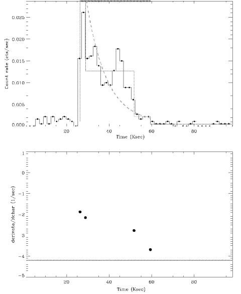
Figure 1: Top: light-curve of a flaring Cygnus OB2 X-ray source, #600 in the list of Albacete Colombo et al. (2007). The histogram shows the light-curve binned in 1800 sec bins. The dotted-line shows the blocks as computed with the MLB algorithm. The first and last blocks are compatible with the characteristic level; the second is classified as “very elevated”; the third and fourth as “elevated” (see text). The blocks identified as belonging to the flare are indicated by a thick solid segment at the top. The dashed line indicates an exponential fit of decay phase. Bottom: ratio between the derivative of the count rate and the characteristic level ${dR\over dt}\cdot{1\over R_{\rm char}}$, calculated at the boundaries of each block. The solid line indicates the threshold (10^-4.2) used for the detection of flares. Note: The observed sequential second flare is an example of the sustained heating and thermodynamics cooling processes competing simultaneously (e.g. Favata & Micela, 2003). This results in longer decay times. MLB compute these cases as single flares.

All the results presented throughout this paper are for CL=99.9%, N_min=1, and D_th=10^-4.2.

3 Flare properties of Cygnus OB2 sources

We applied the MLB algorithm and our operative definition of flare to the 1003 X-ray sources in the Cygnus OB2 region. We detected a total of 147 flares occurring in 143 X-ray sources. This means that about 14.7% of the sources appear to flare during the 100 ksec Chandra observation. We found that 74 of the flaring sources are also definitively variable according to the KS-test (P_ks$\geq$ 99.9%), while an other 25 have 99%$<$P_KS$<$99.9%. For the 48 remaining sources, P_KS$\leq$99%. Most of these sources (32/48$\sim$67%) have less than 40 photons. Given that the confidence level used for the MLB algorithm was 99.9%, this seems to be more efficient than the KS-test in detecting variability, especially in the low-photon statistical regime.

Table 1: X-ray properties of flaring sources in the Cygnus OB2 region. The complete version is available in the electronic edition of A&A

Nx	Identification	Albacete Colombo et al. (2007)				KS-test	MLB analysis
#	2MASS J+	Mass	Phot.	Ex	log(Lx)	log(PKS)	Rchar	Tflr	log(L${}^{\rm peak}_{\rm x}$)	Eflr	$\tau_{\rm E/L}^{\rm meas}$	$\tau_{\rm fit}$
[1]	[2]	[3]	[4]	[5]	[6]	[7]	[8]	[9]	[10]	[11]	[12]	[13]
1	$---------$	$--$	67	3.23	30.80	-4.00	0.158	2.21	32.10	35.62	0.91	0.61
6	20322768+4113169	1.59	216	2.61	31.32	-4.00	0.958	8.18	31.98	35.99	2.87	2.64
8	20322913+4114012	0.48	33	2.62	30.26	-0.59	0.300	0.10	31.46	34.48	0.30	$--$
20	20323249+4113131	2.27	49	2.64	30.65	-2.69	0.145	9.01	31.01	35.46	7.70	$--$
28	20323592+4112505	0.94	43	2.04	30.51	-2.14	0.245	5.03	31.15	35.20	3.06	$--$
33	20323661+4122147	6.83	232	1.93	31.22	-4.00	0.985	12.14	31.74	36.03	5.40	4.45
37	20323751+4117121	0.18	55	2.68	30.68	-4.00	0.104	3.85	31.44	35.55	3.59	$--$
39	20323784+4122087	1.41	91	2.20	30.81	-1.56	0.463	9.87	31.15	35.58	7.43	$--$
43	20323810+4112442	1.19	53	2.74	30.64	-4.00	0.246	3.14	31.38	35.40	2.91	$--$
51	20323989+4113488	0.58	32	1.97	30.23	-2.91	0.127	7.08	30.90	35.19	5.46	$--$
52	20324009+4110346	7.97	156	2.69	31.28	-4.00	0.533	3.72	32.04	35.93	2.14	1.62
54	20324032+4122473	1.16	73	2.68	30.68	-1.06	0.570	1.44	31.50	35.14	1.21	$--$
57	20324063+4111113	0.54	30	2.71	31.05	-2.31	0.125	8.68	30.80	35.19	6.72	$--$
74	20324288+4119148	1.52	89	1.86	30.98	-4.00	0.238	8.08	31.44	35.72	5.25	2.82
81	20324342+4111034	0.60	47	2.20	30.58	-4.00	0.180	5.19	31.15	35.37	4.55	$--$
93	20324492+4115203	2.43	45	2.08	30.99	-1.52	0.288	6.22	30.90	35.13	4.77	$--$
125	20324860+4108117	1.27	121	2.23	30.95	-1.33	1.165	0.13	31.68	34.77	0.34	$--$
135	20325011+4116270	0.52	13	2.18	26.58	-1.48	0.056	3.76	31.74	34.80	0.32	$--$
145	$---------$	$--$	15	2.49	30.43	-2.98	0.046	4.05	30.85	34.94	3.43	$--$
146	$---------$	$--$	27	3.19	30.32	-0.59	0.175	2.21	31.07	34.92	1.94	$--$
159	20325218+4118160	2.83	21	1.79	30.28	-2.12	0.112	4.18	30.83	34.94	3.59	$--$
171	20325351+4120195	0.63	11	3.85	31.99	-0.89	0.016	4.72	30.65	34.89	4.83	$--$
172	20325377+4115134	2.39	219	2.42	31.41	-4.00	0.924	9.29	31.80	36.01	4.47	3.65

Note: Rows refer to a source flare. Col. 1: source numbers according to Albacete Colombo et al (2007). Col. 2: name of 2MASS counterpart. Col. 3-6: source characteristics, i.e. mass of stars, “phot” the net detected photons, “E_x” median photon energy, and “L_x ” X-ray luminosity [erg/s]. Col. 7: logarithm of P_KS. Col. 8 count rate of the characteristic level in units 10^-3 [s^-1]. Col 9: flare duration. Col 10: logarithm of the unabsorbed L_x at the flare peak was computed using CF. Col 11: logarithm of the flare energy (Eq. 3). Col 12: $\tau_{\rm L/E}$=E_flr/L_peak. Col 13: fitted decay time of the flare.

In order to estimate the energy of each flare, E_flr, we multiply the number of flare photons, $N_{\rm ph-flr}$ (=$\sum{(R-R_{char})\Delta T}$), by a counts-to-energy conversion factor, $CF$. This is computed from the total energy released by the source during the observation, i.e. the mean L_x times the exposure time, divided by the number of detected source photons, $N_{\rm ph-src}$:

$$E_{\rm flr}={N_{\rm ph-flr}\over N_{\rm ph-src}}\int_{0}^{T_{\rm exp}}L_{\rm x}(t)\,dt={\overline{L_{\rm x}}T_{\rm exp}\over N_{\rm ph-src}}N_{\rm ph-flr}=CF\cdot N_{\rm ph-flr}\hskip 5.69046pt\cdot$$ (3)

For Cygnus OB2 sources $\overline{\rm L_{\rm x}}$ was computed by Albacete Colombo et al. (2007) using a single count rate for the flux conversion factor. For ONC, although X-ray luminosities from X-ray spectral fits for individual sources are available (Getman et al., 2005), we derived new L_x values, for consistency, using the same approach as was used for Cygnus OB2  . Thus E_flr was obtained in the two cases by multiplying $N_{\rm ph-flr}$ by the relative counts-to-energy CF: 7.52$\times$10³² ergs/ph for the ONC and 7.92$\times$10³³ ergs/ph for Cygnus OB2 .

We thus ignored both the source-to-source and the flare-to-flare variability in X-ray spectra. Given the low photon statistic of the sources and flares, in particular of those in Cygnus OB2 , it is indeed not possible to derive source-specific and flare-specific $CF$s. The dependence of $CF$ on plasma temperature is, however, expected to be small.

3.1 Flare duration and decay times

Most observed flares appear to decay exponentially. We thus approximate their light curves as L_x (t)=L₀e^-t/τ, where L₀ is the peak luminosity and $\tau$ the exponential decay time. The parameter $\tau$ is one of most important observationally accessible since it carries information on the physical conditions of the flaring plasma and on the geometry of its confining magnetic field (Serio et al., 1991; Reale et al., 2004).

Unfortunately, $\tau$ is not easily measured for most of our flares because the photon statistic is insufficient for a reliable exponential fit. In the exponential assumption, the measured energy of a flare, E_flr, which we estimate from the number of photons detected from the beginning of the rise phase (assumed instantaneous) to its detected duration, T_flr, can be written as

$$E_{\rm flr}=\int^{T_{\rm flr}}_{0}L_{\rm 0}\,e^{-t/\tau}dt\,\,\,\,\longrightarrow\,\,\,\,\,{E_{\rm flr}\over L_{\rm 0}}=\tau(1-e^{-{\rm T}_{\rm flr}/\tau})\hskip 5.69046pt\cdot$$ (4)

The additive term $e^{-{\rm T}_{\rm flr}/\tau}$ in Eq. 4 could be understood as a correction factor of $\tau$ in a integration limited by T_flr. Note that the quantity ${E_{\rm flr}\over L_{\rm 0}}$ approaches $\tau$ for T${}_{\rm flr}\gg\tau$. Hereafter, we indicate ${E_{\rm flr}\over L_{\rm 0}}$ as $\tau_{\rm E/L}$. In Fig 2 we illustrate computed flare parameters for a typical flare.

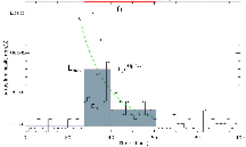
Figure 2: We illustrate flare parameters. Observed flare correspond to source N_x 172. Values of the parameters can be followed in Table 1. Y-axis was converted from the count rate by using CF=7.92$\times$10³³ erg/ph. The shadowed area corresponds to the flare energy. Dashed line refers to the exponential decay fit of the flare. Note: Label “tau” in the equation refers to exponential decay time $\tau$. For flares characterized by three or more blocks, we give fitted $\tau_{\rm fit}$ values in Table 1.

Figure 3: $\tau_{\rm E/L}$($\equiv$E_flr/L₀) vs. T_flr, the measured duration of flares. Filled circles indicate the observationally derived values, E_flr/L_max, for flares detected on Cygnus OB2 stars; vertical error-bars the allowed range of $\tau_{\rm E/L}$ considering the observational biases on L₀: [0.5E_flr/L_max,E_flr/L_max]. Curves show the theoretical loci for exponentially decaying flares (Eq. 4) with different decay times, $\tau$, as labeled on the right-hand side (in hours). Note: Dashed line represents the limit case for which T${}_{\rm flr}\gg\tau$ (Eq. 4), and thus the exponential correction factor ($e^{-{\rm T}_{\rm flr}/\tau}$) vanishes (see text).

In Fig. 3 we plot $\tau_{\rm E/L}$ vs. the time duration of flares, t_flr, both estimated from the MLB analysis. We note in particular that L₀, entering into the calculation of $\tau_{\rm E/L}$, is approximated here with the maximum luminosity of the blocked flare light curve, L_max. For an impulsive rise followed by an exponential decay, this last quantity is by definition smaller than the true peak flare luminosity (i.e. L_max$<$L₀), but typically greater than $\sim$0.5 L₀. The vertical error bars in Fig. 3 reflect the resulting uncertainty on $\tau_{\rm E/L}$: 0.5E_flr/L_max$<$$\tau_{\rm E/L}$$<$E_flr/L_max. We also plot the theoretical loci, calculated from Eq 4, for values of $\tau$ ranging from 1 to 24 hours. A comparison of these theoretical curves with the data points indicates that the observed flares span a wide range of decay times.

We now wish to test the usefulness of $\tau_{\rm E/L}^{\rm meas}$($\equiv$E_flr/L_max) as a measure of the flare’s decay time. For this purpose we have created a large number of simulated light curves assuming the same flare energy distribution found for Cygnus OB2 sources (see §3.2) and for a set of $\tau$ ranging from 2 to 16 hours. We then applied the MLB algorithm and our flare definition to characterize flare properties in the same way as for Cygnus OB2 sources. In Fig. 4 we present histograms of $\tau_{\rm E/L}^{\rm meas}$ and t_flr resulting for simulations with $\tau$ equal to 2, 4, and 6 hours. While t_flr appears broadly distributed, the distribution of $\tau_{\rm E/L}^{\rm meas}$ for simulated flare values peak at the corresponding $\tau$ input value. This suggests that $\tau_{\rm E/L}^{\rm meas}$ may indeed be used as an estimator of $\tau$, with a typical, associated uncertainty $\sigma$($\tau$)$\sim$0.3$\tau$. Columns 12 and 13 of Table 1 give the values of $\tau_{\rm E/L}^{\rm meas}$ for all the 147 flares detected on Cygnus OB2 sources. The median $\tau_{\rm E/L}^{\rm meas}$ is 2.9 hours and 90% of the values are in the [0.5,9] hour range. For 27 flares for which the light curve comprised more than one block we also computed $\tau$ from exponential fits to the block count rates. For these 27 sources, the median $\tau_{\rm E/L}^{\rm meas}$ and $\tau_{\rm fit}$ are both 2.6 hours. The distributions of $\tau_{\rm E/L}^{\rm meas}$ for the whole sample and for the 27 flares with exponential fits and that of $\tau_{\rm fit}$ for the latter sample are all statistically indistinguishable from each other using two-sample Kolmogorov-Smirnov tests (all giving null probabilities $>$16%).

Figure 4: Distributions of the detected flare duration t_flr (dashed lines) and $\tau_{\rm E/L}^{\rm meas}$ (solid lines) for simulated light curves constructed with flares having three different decay times $\tau$: 2,4, and 6 hours. Note that, while the distributions of $\tau_{E/L}^{\rm meas}$ peak at the simulation input values, t_flr appears broadly distributed towards higher values.

3.2 Flare energy distribution

Studies of the solar corona (i.e. Lin et al., 1984; Krucker & Benz, 1998) have found solid evidence of small-scale of continuous flaring. The distribution in energy of these flares was found to follow a power law: dN/dE $\propto$ E^-α, where dN is the number of flares produced in a given time interval with a total energy (thermal and radiated) in the interval [E, E+dE], and $\alpha$ is the index of the power-law distribution (Datlowe et al., 1974; Hudson, 1991).

The total energy released in flares is obtained by integration:

$$E_{\rm tot}=\int^{E_{\rm max}}_{E_{\rm min}}{dN\over dE}\,E\,dE=k\int^{E_{\rm max}}_{E_{\rm min}}E^{1-\alpha}\,dE\approx{k\over\alpha-2}\,E_{\rm min}^{-(\alpha-2)}\hskip 5.69046pt\cdot$$ (5)

where $E_{\rm min}$ and $E_{\rm max}$ are the minimum and maximum allowed flare energies, respectively, $k$ is a normalization factor and in the last passage we assumed $\alpha$$>$2 and $E_{\rm max}$$\gg$$E_{\rm min}$. For $\alpha$$>$2, the integral diverges if $E_{\rm min}$$\rightarrow$0, meaning that the energy released from micro flares ($\sim$10²⁷-10³⁰ ergs) and nano flares ($\sim$10²⁴-10²⁷ ergs) can contribute large amounts of energy to the total emission and eventually explain the whole coronal output (Hudson, 1991). A non-zero value of $E_{\rm min}$ or a flattening of the flare energy distribution at energies is required to keep the total emitted energy finite. The cumulative distribution of flare energies also follows a power law:

$$N(>E_{\rm flr})\propto\int^{\infty}_{\rm E_{\rm flr}}E^{-\alpha}\,dE\propto{1\over\beta}{E_{\rm flr}}^{-\beta}{\rm\,\,\,\,where\,\,\,\beta=\alpha-1}\hskip 5.69046pt\cdot$$ (6)

In the following, we compare the observed cumulative distribution of flare energies with the above theoretical distribution in order to constrain the slope, $\alpha$. More precisely, we consider the observed frequency of flares per source vs. the minimum flare energy, i.e. N($>E_{\rm flr}$) divided by the number of sources in our sample and by the duration of the observation. Note however that, even if the simple power law model is correct, the observed distributions will flatten at low energies due to an observational bias; i.e., small events are missed by our flare detection process. Above a certain threshold energy, E_cut, however, our list of detected flares will probably be complete.

Other than the sensitivity bias, a simple cumulative distribution of flare energies can also be biased by the effect of overlapping flares. More specifically, the “effective” time available for the identification of flares with a given energy is reduced by the presence of larger ones, usually known as dead-time correction. This effect is generally small, given the low frequency of detectable flares. We correct for this bias, however in the derivation of the frequency of flares by assuming that the time available for detect flares with a given energy is reduced by the sum of the durations of more energetic flares (see, Audard et al., 2000; Stelzer et al., 2007). Figure 5 (upper panel) shows, for the Cygnus OB2 X-ray sources, the dead-time-corrected cumulative distribution of flare energies, in units of flares per source per ksec.

Figure 5: Upper panel: Frequency of flares (flares per source per ksec) with energy above E_flr vs. E_flr, for Cygnus OB2 sources as derived from our 100 ksec Chandra observation. Middle panel: Maximum Likelihood estimate of the power-law index that better approximate the distribution for flare energies above E_flr. Three dashed lines, from top to bottom, ref fer to $\beta$-values 1.1, 1.0, 0.9, respectively. Bottom panel: probability, according to the KS test, that a power law with best-fit index as given in the middle panel, is compatible with the observed distribution for energies above E_cut.

We use the maximum likelihood method described by Crawford et al. (1970) to determine E_cut, i.e. the minimum energy above which the distribution is compatible with a power law, and $\beta$, the best-fit slope of the power law. The details of the statistical analysis can also be followed in Stelzer et al. (2007).

In summary, we have computed, as a function of E_flr, the maximum-likelihood slope, $\beta$(E_flr), of the cumulative distribution of flares with energies higher than E_flr. Alongside $\beta$(E_flr) we also used the Kolmogorov-Smirnov test to computed P_KS(E_flr), i.e. the probability that a power law with index $\beta$(E_flr) is indeed compatible with the observed distribution. The two functions are shown in the middle and bottom panels of Fig. 5. We chose E_cut=10^35.1 ergs s^-1 with respect to the maximum of P_KS ($\sim$30%). This leads in an index $\beta$$\approx$1.1$\pm$0.1. Note that further increasing E_cut means $\beta$(E${}_{\rm flr})$ reaches a plateau, confirming the compatibility of the observed flare energy distribution, above E_cut, with a power law.

In spite of our statistical analysis, our estimation of $\beta$ and E_cut from the observed energy flare distribution could still be biased by the limited exposure time of the observation precluding the detection of a fraction of the longer flares. This bias could mainly affect the high-energy tail of the observed flare energy distribution of Cygnus OB2 sources. Unfortunately, with our 100 ksec observation, we are unable to quantify the degree of this incompleteness.

In the extraordinarily long COUP observation ($\sim$850 ksec), however, this bias may be considered negligible. In §4 we present a re-analysis of the COUP data aimed at addressing this issue and at comparing the flare frequency of Cygnus OB2 stars with those of the ONC. First, however, we continue to discuss the issue of the frequency of flares.

3.3 Flare frequency

The low/intermediate-mass, X-ray-detected stellar population within the Cygnus OB2 region covered by our Chandra observation counts, excluding 26 OB stars, 1003-26=977 likely members (Albacete Colombo et al., 2007). We exclude the OB stars from our statistics because their X-ray emission is mostly unrelated to magnetic activity. Our MLB analysis detected a total of 147 flares during the 100 ksec observation. The average flare frequency (f_flr) is thus approximately 1 flare in $\sim$664 ksec. Considering only flares with energies above our completeness limit, E_cut=10^35.1 erg, the flare frequency is reduced to f_flr=1/1320 ksec^-1.

The flare frequency can, however, be expected to be a function of source photon statistic, because of the combined effects of the limited sensitivity of our flare detection procedure and of the likely dependence of the flare intensity distribution on source brightness. Table 2 reports the flare frequencies calculated for a sub sample of stars with different minimum numbers of detected photons. Figure 6 also shows the full distributions of flare frequencies computed for different ranges of the source’s photon statistics. Given the bias against the detection of low-energy flares, the flare frequencies for different sub samples are more directly comparable when considering only those flares with energies above our completeness limit, E_flr$>$E_cut. This quantity is given in the last column of Table 2.

Figure 6: Flare frequency vs. minimum energy (as in Fig. 5) for source sub samples with different minimum numbers of detected source photons (N_ph), as indicated beside each curve. The dashed vertical line marks our flare detection detection completeness limit determined in § 3.2. Note: For sources with a similar N_ph, differences in the energy of the flare are due to their respective exponential decay times ($\tau$).

Table 2: Flare frequency for stars with different photon statistics

Min	Nsrc	Nflr	fflr [ksec-1]
counts	in sample	in sample	total	comp.∗
1	977	147	1/664	1/1320
10	928	143	1/644	1/1254
20	787	140	1/562	1/1063
30	630	132	1/477	1/863
40	531	114	1/465	1/748
50	434	102	1/425	1/629
80	265	74	1/358	1/416
120	134	44	1/304	1/352
150	78	35	1/222	1/252
180	47	33	1/142	1/162
250	13	12	1/108	1/108

The 26 X-ray sources identified with OB stars were excluded from the analysis of flare frequencies. Note: $\ast$ indicates flare frequencies (f_flr) with energies above our completeness limit (i.e. log E_flr$>$35.1 ergs).

Because of the strong dependence of the observed flare frequency on the sensitivity of the observation and on the intrinsic brightness of the X-ray sources, a direct comparison with previous determinations for members of other SFRs is difficult. For example, the flare frequency (f_freq) computed for the PMS stars in the Taurus molecular clouds (TMC) by Stelzer et al. (2007) is 1/200 ksec^-1, much higher than our frequency for the whole Cygnus OB2 sample. The difference may largely be explained as a sensitivity effect, given that the TMC is $\sim$11 times closer than Cygnus OB2 and that the observation were performed with a more sensitive instrument (XMM-Newton instead of Chandra ). Note that for a “complete” sample of flares (i.e. those with E_flr$>$10³⁵ ergs) Stelzer et al. (2007) find f_flr$\sim$1/770 ksec. During the COUP observation in the ONC Wolk et al. (2005) observe 41 flares in a sample of 27 solar-mass stars implying f_flr$\sim$1/650 ksec^-1. This figure reduces to f_flr$\sim$1/1150 ksec^-1 if we only consider flares with energies above the completeness limit estimated by Stelzer et al. (2007), i.e. 10^35.3 ergs.

Obviously, all these rates of flaring are not easily compared because of the different instruments, exposure times, sensitivity, and the resulting completeness limits for the observations. The availability of the COUP data gives us the opportunity to re-analyze this observation consistently with Cygnus OB2 data, so as to minimize this differences. We give details of this analysis in the next section.

4 The analysis of the COUP data

The COUP data set combines six nearly consecutive exposures of the ONC, spanning 13.2 days (1140 ksec) with a total exposure time of 850 ksec (9.8 days). The observation was taken with the ACIS-I camera onboard Chandra . A complete description of the COUP data analysis and source detection procedures can be found in Getman et al. (2005). Here we make use of the 1616 source event files.

To understand the bias introduced by the limited exposure time of our 100 ksec Cygnus OB2 observation, we present the analysis of the entire 850 ksec COUP observation here, as well as that of five different 100 ksec segments. As anticipated in §2, the 5$\times$100 ksec segments (Seg. 1,2,3,4, and 5) were defined arbitrarily, but avoided time gaps in the COUP observation. Figure 7 shows, as an example, the light curve of COUP source #1276. The horizontal segments labeled as “Seg. 1-5” indicate the time intervals for which we independently performed the flare analysis and we also indicate flares detected in the whole observation and in the 5 segments separately. Because the count rates obey Poison statistics, the maximum amplitude of fluctuations increases with exposure time. This implies that the statistical significance of a real signal (e.g. a flare) is higher when considering a shorter time interval. The MLB algorithm, applied with the same significance threshold (99.9% in our case) to the whole observation and to the shorter segments, can therefore yield different results. In particular, as exemplified in Fig. 7, faint flares may remain undetected in the former case (seg. 3), and consecutive flares may be detected as a single event (seg, 1 and 2).

Inspection of the segmented light curves led to excluding three sources (COUP #9, #828 and #1462) from the following considerations, they lie close to the edges of the ACIS-I CCDs: because of the wobbling of Chandra , the light curves of these sources show high frequency variations at the wobbling period, leading to the spurious detection of a large number of flares.

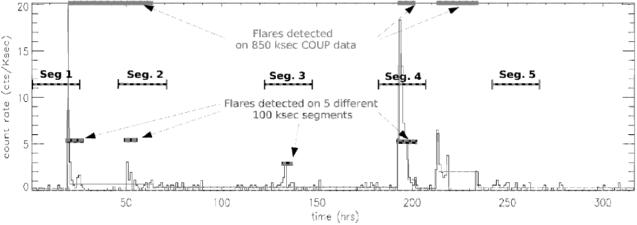
Figure 7: Example of MLB flare detection for COUP source #1276. The result of the MLB algorithm applied to the whole observation is overlaid on the binned light curve. The three thick horizontal segments on the top indicate flares detected using this representation. The four thick segments on the bottom instead indicate the flares detected by applying the MLB algorithm to the 5 different 100 ksec time intervals, with latter indicated by the thinner segments labeled “Seg. 1-5”. Note: time is given in hours from the beginning of the observation.

Figure 8 shows the rate of flaring vs. minimum flare energy for the entire 850 ksec COUP observation, for each of the five independent 100 ksec COUP data segments, and for the combined flare population of the 5 segments. This curve, while maintaining the same properties with respect to observational biases, such the 5 curves for the single segments, improves the statistics and allows a more robust estimation of the mean flare frequency and of slope $\alpha$.

Results of the MLB analysis for the COUP data are presented in Table 3. We report the following for each of the above data selections: N_src, the total number of sources that show flare activity (row 1); N_flr, the total number of detected flares (row 2); 1/f_flr, the inverse of the single-source flare frequency, i.e. the number of flares divided by the total observing time in ksec (row 3); E_cut, the flare energy threshold above which flare detection is considered statistically complete (row 4); N${}^{\rm comp}_{\rm flr}$, the number of flares with energies above E_cut (row 5); 1/f${}^{\rm comp}_{\rm flr}$, the inverse of the flare frequency for flares with energies above E_cut (row 6); $\alpha$, the slope of the power law that characterizes the flare energy distribution above E_cut (row 7); $\sigma(\alpha)$, the 1$\sigma$ uncertainty on $\alpha$ (row 8). Columns 2 to 6 give results for the analysis of the 5$\times$100 ksec segments, column 7 the results for the summed 5$\times$100 ksec segments, and column 8 the results for the analysis of the entire 850 ksec COUP observation.

Table 3: Statistics of X-ray flares in the ONC

COUP	5 $\times$ 100 ksec segments						850
Results	Seg1	Seg2	Seg3	Seg4	Seg5	Total	ksec
Nsrc	125	111	110	111	127	584	640
Nflr	128	112	112	115	130	601	954
1/fflr	1253	1432	1382	1395	1233	1334	1429
logEcut	34.6	34.6	34.5	34.6	34.5	34.7	35.6
N${}^{\rm comp}_{\rm flr}$	75	63	79	62	89	313	246
1/f${}^{\rm comp}_{\rm flr}$	2138	2546	2030	2587	1802	2562	5542
$\alpha$	1.9	1.9	1.85	1.9	1.9	1.9	2.05
$\sigma(\alpha)$	0.1	0.1	0.1	0.1	0.1	0.1	0.15

Notes: 1/f_flr is in ksec, E_cut in erg. COUP sources #9, #828, and #1462 were excluded from the analysis (see text).

For the 1616 COUP sources observed for the whole 850 ksec exposure, we found that detection of flares is complete for events with log(E_flr)$>$35.6, and the cumulative distribution follows a power law with index $\alpha$$\sim$2.05$\pm$0.15, in agreement with results obtained by Stelzer et al. (2007) for solar-mass stars (i.e. log(E_flr)$>$35.3 and $\alpha$$\sim$1.9$\pm$0.2). For the 100 ksec segments, we obtained $\alpha$=1.9$\pm$0.1, which is within $\sim$1$\sigma$ of the result obtained for the whole observation. Our analysis thus indicates that the slope of the flare energy distribution obtained from a 100 ksec observation is statistically consistent with what is obtained from a much longer (850 ksec) observation. The flare frequencies obtained from the shorter exposures are, however, significantly reduced. An inspection of the results of the flare detection processes reveals that many flares are missed in the short exposures either because the segment does not include the phases characterized by a high time derivative (the rise phase and the beginning of the decay) or, in a considerable number of cases, because the characteristic level is not observed and/or correctly determined. In some other cases, moreover, the flare is detected, but a large part of the flare falls outside the segment, thus underestimating its energy.

Figure 8: Flare rate vs. minimum flare energy for the ONC X-ray sources observed by COUP, as determined from flares detected in: $i$- each of the five selected 100 ksec segments of the COUP data (dashed lines), $ii$- all the five segments (thin solid line), $iii$- the whole 850 ksec COUP exposure (thick solid line). Note that, as discussed in the text, more low-energy flares are detected in the 100 ksec segments with respect to the whole observation, but a significant fraction of the longer/more energetic ones are missed.

4.1 Comparing the ONC with the Cygnus OB2 region

Figure 9: Rate of flaring vs. minimum flare energy for: $i$- the Cygnus OB2 sources with mass $\geq$ 1 M_⊙ observed during our 100 ksec observation (thick solid line), $ii$- all the COUP sources observed during the five 100 ksec segments of the COUP observation (dashed line), $iii$- COUP sources with mass $\geq$ 1 M_⊙ in the five 100 ksec segments (thin solid line).

Due to the small difference in age between the ONC (1 Myr) and Cygnus OB2 (2 Myr), we expect the X-ray properties of stars in the two regions to be similar. Albacete Colombo et al. (2007) indeed found similar average X-ray emission levels. For the comparison of flare properties to be meaningful, we must consider results obtained from observations of the same temporal length. For the ONC we therefore consider the results from the the analysis of the five 100 ksec segments. Moreover, given the dependence of the X-ray luminosity on stellar mass and the relation between source luminosity and flare frequency (§3.3), a meaningful comparison between the two regions should only consider sources in a similar range of mass. We therefore computed the flare energy distribution for the 92 ONC stars in the catalog of Getman et al. (2005) with masses $\geq$ 1M_⊙, i.e. roughly the lower mass limit of X-ray detected Cygnus OB2 stars (Albacete Colombo et al., 2007). Figure 9 compares this distribution with that of the Cygnus OB2 sources with mass $\geq$1M_⊙, both normalized to yield the average single-source rate of flaring.

We analyzed the flare energy distribution for ONC sources with M $\geq$ 1M_⊙ using the same statistical procedure as described in § 3. We find that, for E_flr$\geq$10^35.2 ergs, the distributions for Cygnus OB2 and ONC sources with masses higher than 1M_⊙ (see thick and thin lines in Fig. 9, respectively) are compatible with a power law with index $\beta$=1.1$\pm$0.1 (i.e. $\alpha$$\sim$2.1$\pm$0.1). We conclude that the flare statistics of the Cygnus OB2 and ONC stars are very similar.

5 Summary and conclusions

We conducted a systematic analysis of flare variability in the soft X-ray band of the young stars in the Cygnus OB2 star-forming region. For this purpose we analyzed the lightcurves of 1003 X-ray sources detected in a 100 ksec Chandra observation. For comparison we also used the same method to analysis of lightcurves of the 1616 X-ray sources detected in the ONC with the 850 ksec observation of the Chandra Orion Ultra-deep Project. To compare the results for the two regions, avoiding biases due to the different exposure times, we also analyzed, independently, five 100 ksec long segments of the COUP observation.

Flares were detected using the MLB algorithm. A total of 147 flares were detected in the lightcurves of 143 Cygnus OB2 sources. In the ONC, 954 flares were detected on 640 sources in the analysis of the whole 850 ksec observation, while 601 flares were detected on 584 source in the analysis of the five 100 ksec segments.

For each flare we estimated the emitted energy, E_flr, and the peak luminosity, L_peak. Backed by the analysis of extensive sets of simulated lightcurves, we suggest that the ratio E_flr/L_peak can be considered a reasonable estimate of the flare decay-time, $\tau$. This is particularly useful for weak flares, for which a fit to the light curve is not possible. The 147 flares in our Cygnus OB2 sample have a wide range of decay times from $\sim$0.5 hours to $\sim$10 hours, with a median of 2.9 hours. For the 27 flares that are bright enough, we fitted the decay phase with an exponential finding consistent results: a median $\tau$ of 2.6 hours, and a distribution compatible with that of the whole sample.

We find that Cygnus OB2 and ONC flare energy distributions display high-energy tails described by a power law (dN/dE$\propto$E^-α). For energies below a given E_cut, the distributions flatten as a result of the incomplete detection of faint flares. For Cygnus OB2 sources, we obtain E_cut=10^35.1 ergs and $\alpha$=2.1$\pm$0.1. This slope agrees with the range of values found in previous studies of solar and stellar flares (Güdel et al., 2003; Stelzer et al., 2007) and gives support to the micro-flare hypothesis for the explanation of the observed X-ray emission and for the heating of corona (Hudson, 1991).

The average frequency of flares detected on any given Cygnus OB2 source during our 100 ksec observation is $\sim$1/664 ksec^-1. It reduces to $\sim$1/1320 ksec^-1 when considering only flares with E_flr$>$E_cut=10^35.1 ergs, i.e. those for which detection is likely to be complete. It is, moreover, important to stress that our results, even for flares with energies higher than the “completeness limits”, critically depend on the flare detection method and on the duration of the X-ray observation.

We investigated this point using the 850 ksec COUP data set, as well as for five distinct 100 ksec segments of the same observation. The frequencies as a function of minimum flare energy derived in the two cases are significantly different: the short exposures indeed hinder the detection of long and (usually) energetic flares, often because it is not possible to correctly determine the “characteristic level”, which is instead clearly observed in the longer exposure. The “completeness limits”, E_cut, above which the flare energies appear to follow power law distributions, are also different for the two cases: $10^{35.6}$ and $10^{34.6}$ egrs for the 850 ksec and the 100 ksec observations, respectively. The slopes of the power laws, $\alpha$, are however notably similar, respectively 2.05$\pm$0.15 and 1.9$\pm$0.1, which are compatible with each other and with the slope of the Cygnus OB2 distribution within $\sim$1$\sigma$.

For the ONC stars we considered the analysis of the 100 ksec segments. To compare stars with similar intrinsic X-ray luminosities, we restricted the sample to stars with masses higher than 1 M_⊙, i.e. roughly the completeness limit of our Cygnus OB2 observation. We find that the stars in the Cygnus OB2 and ONC regions have indistinguishable X-ray flare properties.

Finally, we confirm that comparison of flare frequencies is only allowed if observational limitations and data analysis are performed in a single and homogeneous way. Contrary to this result is just the determination of the slope of the power-law distribution, which is not critically influenced by the length of the observation.