The public goods game on homogeneous and heterogeneous networks: investment strategy according to the pool size

Abstract

We propose an extended public goods interaction model to study the evolution of cooperation in heterogeneous population. The investors are arranged on the well known scale-free type network, the Barabási-Albert model. Each investor is supposed to preferentially distribute capital to pools in its portfolio based on the knowledge of pool sizes. The extent that investors prefer larger pools is determined by investment strategy denoted by a tunable parameter $\alpha$, with larger $\alpha$ corresponding to more preference to larger pools. As comparison, we also study this interaction model on square lattice, and find that the heterogeneity contacts favors cooperation. Additionally, the influence of local topology to the game dynamics under different $\alpha$ strategies are discussed. It is found that the system with smaller $\alpha$ strategy can perform comparatively better than the larger $\alpha$ ones.

I introduction

The evolution of cooperation among unrelated individuals is one of the fundamental problems in biology and social sciences vonNeumann ; MaynardSmith ; HauertScience2002 . A number of mechanisms have been suggested which are capable of supporting cooperation in the absence of genetic relatedness. Most notably, this includes repeated interactions and direct reciprocity Trivers ; Axelrod , indirect reciprocity Alexander ; Nowak3 ; Nowak4 , punishment EFehr ; Clutton-Brock , spatially structured populations Nowak1 ; GSzabo2 ; Hauert2 ; Szabo ; HauertScience2002 , or voluntary participation in social interactions Szabo ; HauertScience2002 ; Hauert4 ; Wu1 .

The public goods game (PGG), which attracted much attention from economists, is a general paradigm to explain cooperative behavior through group interactions JHKagel . In this game, the defectors who do not contribute, but exploit the public goods, fare better than the cooperators who pay the cost by contributing. Thus, the defectors have a higher payoff. If more successful states spread, cooperation will vanish from the population, and the public goods along with it. By considering the fact that who-meets-whom is determined by spatial relationships or underlying networks, Szabó and Hauert et al. have recently studied evolutionary PGG in spatially structured populations bound to regular lattices Szabo ; Hauert ; HauertScience2002 as well as the well-mixed population HauertScience2002 ; Hauert4 ; Hauert3 ; Hauert5 . In these work, the effects of compulsory and voluntary interactions of agents are also discussed. Several factors such as the voluntary participation Hauert , and small density of population Hauert3 , which result in small size of interaction group, are found to be capable of boosting cooperation.

However, it has been recognized that regular graphs constitute rather unrealistic representations of real-world network of contacts (NoCs), in which local connections (spatial structure) coexist with long-range connections (or shortcuts). Also, connections in real-world networks are heterogeneous, in the sense that different individuals have different numbers of neighbors with whom they interact. Indeed, these features have been recently identified as characteristic of a plethora of natural, social and technological networks Dorogotsev2003 ; Barabasi1999 ; AlbertBarabasi2002 , which often exhibit a power-law dependence on their degree distributions. In addition, it is well accepted that the heterogeneity of network often plays crucial roles in determining the dynamics May2001 ; Boccaletti ; Santos2005 . Therefore it is worth investigating the public goods interactions on scale-free network.

In this paper, we propose an extended PGG model to study the evolution of cooperation and investment behavior upon heterogenous networks. It is known that, in order to reduce risk, investors may take a portfolio consisting of wide variety of joint enterprise portfolio . In the viewpoint of investors, some enterprise may be more attractive than others, i.e., there exists heterogeneity of attractiveness. In our previous work, we have studied the the effect of heterogeneous influences on the evolution of cooperation in the prisoner’s dilemma game Wu2 ; Wu3 ; Guan . Here, in the framework of PGG, we will consider the effect of heterogeneity of common pools (which we call pools’ “attractiveness” $\mathcal{A}$) on investors. In our model, investors having public goods interactions occupy the vertices of the underlying network, with the edges denoting interactions between them. Investors are assumed to be aware of the sizes of pools, based on which pools’ attractiveness can be estimated. The attractiveness of one given pool also depends on the investment strategy $\alpha$ of the system, which regulates the extent of investors’ preference to large pools. It will be shown that, compared with the homogeneous network, the heterogeneous graphs generated via the mechanisms of growth and preferential attachment (PA) can distinctively favor cooperation, where, in addition, smaller $\alpha$ strategy favors cooperation more than larger $\alpha$ strategy.

II our model

Investors in our model are arranged on certain kind of underlying network and interact only with their immediate neighbors. A given investor $j$ acts as an organizer of the common pool $j$ with size $k_{j}+1$, where there occurs the PGG involving $j$ itself and its neighbor investors. Here, $k_{j}$ is the degree of $j$. Meanwhile, investor $j$ will participate in the $k_{j}+1$ pools which we named the ‘portfolio’ of $j$ including $k_{j}$ pools organized by its neighbors, and the one pool by itself. The common pool $j$ accumulates capital from all its participant investors, and then equally shares the profit to them. We assume that investors have the capacity for learning the sizes of pools in their own portfolio, which enable them to discriminate pools by estimating the attractiveness quantitatively. The value of a given pool $i$’s attractiveness to investors is $\mathcal{A}_{i}=(k_{i}+1)^{\alpha}$, with the real number $\alpha$ denoting the investment strategy of the system, which regulates the extent of investors’ preference to larger pools. We can see that, the larger the $\alpha$ is, the more attractive the large pools will be. The total amount of capital distributed by a cooperator (state $s=1$) is normalized to unity, while that of a defector (state $s=0$) is zero, which implies that defector withhold its investment to free ride the other investor’s contributions. Investors’ capital will be distributed to pools proportional to the attractiveness. Thus, the amount of capital investor $j$ distributes to one of its pool $i$ at time $t$ is,

$$D_{ji}(t)=\frac{\mathcal{A}_{i}\cdot s_{j}(t)}{\sum_{l\in\mathcal{N}(j)}\mathcal{A}_{l}},$$ (1)

where $\mathcal{N}(x)$ is the community composed of the nearest neighbors of $x$ and itself, and $s_{j}(t)$ is the state of investor $j$ at time $t$. Investors will equally distribute their capital into pools in portfolio when $\alpha=0$. They invest large fraction of capital into larger pools for the case of $\alpha>0$, or into smaller pools for the case of $\alpha<0$. If investor $j$ is a defector [$s_{j}(t)=0$], it distributes nothing to its pools, and thereby $D_{ji}(t)=0$.

Then, the amount of capital the pool $i$ accumulates at time $t$ can be written as,

$$C_{i}(t)=\sum_{j\in\mathcal{N}(i)}D_{ji}(t)=\sum_{j\in\mathcal{N}(i)}\frac{\mathcal{A}_{i}\cdot s_{j}(t)}{\sum_{l\in\mathcal{N}(j)}\mathcal{A}_{l}}$$ (2)

We can express Eq. (2) in terms of the following matrix equation,

$$\vec{C}(t)=A\vec{S}(t):=\begin{pmatrix}a_{11}&\dots&a_{1n}\\ a_{21}&\dots&a_{2n}\\ {3}\\ a_{n1}&\dots&a_{nn}\\ \end{pmatrix}\cdot\begin{pmatrix}s_{1}(t)\\ s_{2}(t)\\ \dots\\ s_{n}(t)\end{pmatrix}$$ (3)

where the elements of the matrix $A$ are given by,

$$a_{ij}=\begin{cases}{\mathcal{A}_{i}}/{\sum\limits_{l\in\mathcal{N}(j)}\mathcal{A}_{l}}&j\in{\mathcal{N}(i)}\\ 0&\text{otherwise}\end{cases}.$$ (4)

After the foresaid investing period, the total amount in the pools multiples by a constant factor $r$, namely, the interest rate on the common pools. For simplification, we assume that the profit of each common pool is then equally shared to all participants irrespective of their individual contribution. Thus the aggregate payoff of agent $i$ after one generation is,

$$P_{i}(t)=\sum_{j\in\mathcal{N}(i)}\frac{r\cdot C_{j}(t)}{k_{j}+1}$$ (5)

It can be written as $\vec{P}(t)=rBA\vec{S}(t)$, where the $n\times{n}$ matrix $B$ has element $b_{ij}$ as,

$$b_{ij}=\begin{cases}{1}/({k_{j}+1})&j\in{\mathcal{N}(i)}\\ 0&\text{otherwise}\end{cases}.$$ (6)

Taking into account the unity capital initially distributed by cooperator, the total returns of investors can be written as $\vec{R}=\vec{P}-\vec{S}$.

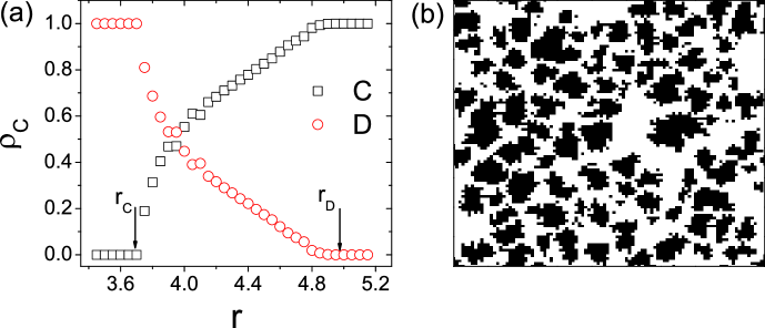
Figure 1: Average frequencies of cooperators and defectors as a function of interest rate $r$ (a), and typical snapshot of the $30\times 30$ square lattice with $r=3.8$ (b). Black refers to cooperators, and white to defectors. The results in (a) are averaged over $40$ realizations. The $r_{C}$ ($r_{D}$) indicates the value of $r$ where cooperators (defectors) vanish.

The return $\vec{R}$ obtained in PGG interactions denotes the reproductive success, i.e., the probability that one neighbor will adopt the agent’s state. In order to maximize total returns, investors update their states after each round of game according to the following rule: Investor $i$ selects one of its neighbor investor $j$ with equal probability. Given the total returns ($R_{i}$ and $R_{j}$) from the previous round, $i$ adopts neighbor $j$’s state with probability GSzabo2 ; Szabo :

$$W[s_{j}\rightarrow{s_{i}}]=\frac{1}{1+exp[(R_{i}-R_{j}+\tau)/\kappa]}$$ (7)

where $\tau>0$ denotes the cost of state change, and $\kappa$ characterizes the noise introduced to permit irrational choices. For $\kappa=0$ the neighboring state $s_{j}$ is adopted deterministically provided the payoff difference exceeds the cost of state change, i.e., $R_{j}-R_{i}>\tau$. For $\kappa>0$, states performing worse are also adopted with a certain probability, e.g., due to imperfect information. Following the previous work Szabo , we simply fix the value of $\kappa$ to be $0.1$.

III simulation results

First, we briefly consider the extended PGG dynamics upon square lattice with periodic boundary conditions, where the strategy $\alpha$ does not affect the capital distribution because of the degree homogeneity. The dynamics starts from the random arrangement of investors’ states either as cooperators or defectors. In Fig. 1(a), we show the average equilibrium frequencies of cooperators and defectors as a function of interest rate $r$. It is expectable that, the curve shows a growth in the frequency of cooperators with increasing values of $r$. Below the threshold value $r<r_{C}$ cooperators quickly vanish, whereas for high $r>r_{D}$ defectors go extinct. For intermediate $r$ the two states coexist in dynamical equilibrium. The subscript $S$ of $r_{S}$ refers to the vanishing state. Just as was found in Refs. GSzabo2 ; Nowak1 ; Szabo , the snapshot of the dynamics (Fig. 1(b)) shows that cooperators persist by forming clusters and thereby minimizing exploitation by defectors.

Let us now consider the evolutionary dynamics of PGG upon the Barabási-Albert (BA) model Barabasi1999 ; AlbertBarabasi2002 . It means that different investors in this system will have portfolios consisting of different number of pools. Also, some pools may absorb capital from many investors, whereas other pools may absorb from much less investors. In addition, the size of pools exhibits a scale-free distribution as the degree of the underlying network, which result in very different values of attractiveness. Here, we want to point out that, although larger pools have more investors, whether they can accumulate more capital than the smaller pools still depends on the investment strategy, preferring the smaller pools ($\alpha<0$), the larger pools ($\alpha>0$), or equally distributing investment ($\alpha=0$).

Numerical simulations are performed in a system of $N=4000$ investors located on a BA network with average connectivity fixed as $4$ which is the same as the square lattice. That is, the network grows from a completely connected network with $m_{0}=5$ vertices, and at every time step a new vertex with $m=2$ edges is added (the construction of the BA network can refer to Refs. Barabasi1999 ; AlbertBarabasi2002 ). Fig. 2 shows the average equilibrium frequencies of cooperators with different $\alpha$ strategies on BA networks. One can notice that, no matter what the strategy $\alpha$ is, the qualitative feature of frequencies of states remain unchanged for the BA network. Again three domains are observed: defectors dominate for low $r<r_{C}$, co-existence for intermediate values of $r$ and homogenous cooperation for high $r>r_{D}$. However, we find that the heterogeneous structure distinctly favors cooperators, because the $r_{D}$ (where defectors vanish) for the BA networks are much smaller than that for lattice (see Fig. 1). Furthermore, we notice that the system with smaller $\alpha$ strategy would behave better than that with larger $\alpha$, which implies that cooperation are rendered more attractive when investors prefer smaller pools rather than larger ones.

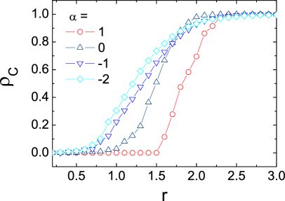
Figure 2: Average frequency of cooperators as a function of interest rate $r$ with investment strategy $\alpha=-2$, $-1$, $0$, and $1$, respectively. Parameters: $\tau=0.1$ and $\kappa=0.1$.

IV analysis and discussions

We can understand the above-mentioned simulation results by the following analysis. From individual perspective, the unit investment contributed by one cooperator $i$ will be returned to the system as $r$ payoff after each round of game. The amount of payoff returned to $i$ itself can be written as,

$$P_{ii} = \sum_{j}\frac{r\cdot D_{ij}(t)}{k_{j}+1}$$ (8)

$$= r\cdot{\frac{\sum_{j}[1/(k_{j}+1)]\cdot{\mathcal{A}_{j}}\cdot{s_{i}(t)}}{\sum_{j}\mathcal{A}_{j}}}$$

$$\equiv r\cdot{s_{i}(t)}\cdot{L_{\alpha}}.$$ (9)

Here, $j\in{\mathcal{N}(i)}$, and $L_{\alpha}$ denotes the weighted average of $1/(1+k_{j})$ with $\mathcal{A}_{j}$ as weight factor. Thus, how much one cooperator can benefit itself from its own unity investment depends on interest rate $r$, investment strategy $\alpha$, as well as its local topology including the degrees of its own and its neighbors. For a given investor, the temptation to defect can be measured in terms of $1.0-P_{ii}$, which is actually independent of other investors’ states. Note that for $r>1/L_{\alpha}$ the social dilemma raised by the PGG is relaxed in the sense that each unity investment has a positive net return, and therefore investor can pay off better when adopting cooperation rather than defection. Here, $1/L_{\alpha}$ in our extended PGG model in fact corresponds to the group size in the original PGG model HauertScience2002 . For the networks with homogeneous degree $k$, $1/L_{\alpha}$ returns to $k+1$ as the value of group size, while for heterogeneous network, the values of $1/L_{\alpha}$ are various for different investors. We give the illustration of $P_{ii}$ on BA network in the case that all investors adopt cooperation ($\vec{S}=1$). The interest rate $r$ is set as $1.0$ so that $L_{\alpha}=P_{ii}$.

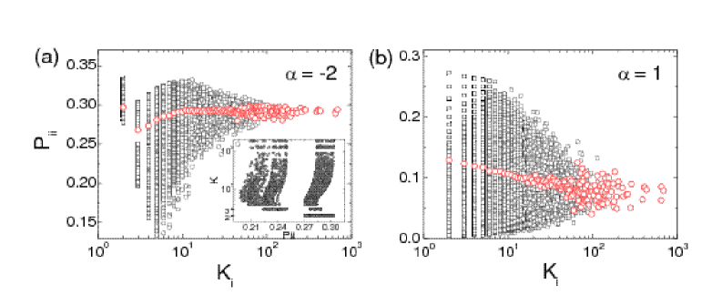
Figure 3: The $P_{ii}$ of investors as a function of their degree $k_{i}$ (square), and the average $P_{ii}$ over investors with given degree (dot) with $\alpha=-2$ (a), and $\alpha=1$ (b), respectively. The network is a BA model with $N=10^{5}$ and $m=2$.

In Fig. 3, we show $P_{ii}$ of investors as a function of their degree $K_{i}$, with investment strategy $\alpha=-2$ (a) and $\alpha=1$ (b). It is noteworthy in the figures that investors with the same degree may have wide range of $P_{ii}$, which reveals the great diversity of agents’ individual local connection. One can notice from the average values with $\alpha=-2$ that the $P_{ii}$ of investors with large degree and smallest degree ($k=2$) is similar, while that of the intermediate degree investor, especially the $k=3$ investor, is comparatively small. It is known for BA model that, those agents with degree $k=m$ are latterly added following degree-PA mechanism, and thereby more probably to have large degree neighbors. When investor prefers small pools ($\alpha<0$) the investor $i$ with degree $k=2$ would distribute most of its investment to pool $i$, and then gain $1/3$ of the profit, with the largest amount approximately equal $1/3$ [see Fig. 3(a)]. In contrast, agents with $k=3$ still have a neighbor which is younger than them, thus more likely to be of small degree. The investor $j$ with $k=3$ will distribute part of its capital $c$ (the amount between $0.0$ and $1.0$) to its own pool $j$ and then gain $c/4$, with the remained capital gain less than $(1-c)/3$ profit. Therefore, generally speaking, the $P_{ii}$ of $k=3$ investor is smaller than that of $k=2$ investor. In the inset of Fig. 3(a), we plot the relations of each $k=3$ investors’ $P_{ii}$ with its $3$ neighbors’ degree $k^{\prime}$. One can notice that, for the intermediate degree investors, the separated range of $P_{ii}$ [see Fig. 3(a)] is closely related to the $k^{\prime}=m$ neighbor. Those investors with neighbors’ minimum degree $k^{\prime}_{min}=2$ would have larger $P_{ii}$, while those with $k^{\prime}_{min}\geq 3$ are comparatively small ($P_{ii}<1/4$). In addition, the large degree investors almost deterministically have $k^{\prime}_{min}=2$ neighbor pools, which pay them off with more profit than the large pools. Thus the corresponding ranges of $P_{ii}$ are not separated, and the average values are around $0.3$ for large degree investors. In addition, when $\alpha=1$ [see Fig. 3(b)], investors are likely to distribute most capital into large pools. The decrease of the average $P_{ii}$ with agent’s degree can be attributed to investor’s increasing number of large pools, which shares the profit to more (other) investors rather than returning to $i$ itself. From the former analysis, one gets that local topology of networks has significant impact on PGG dynamical process.

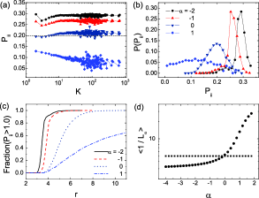
Figure 4: (a) Average $P_{ii}$ over given degree investors under different investment strategies. The strategies from top to bottom respectively are $\alpha=-2$, $-1$, $0$, and $1$. And (b) the corresponding probability distribution of $P_{ii}$. The interest rate $r$ is set as $1.0$. (c) The fraction of investors whose $P_{ii}$ are larger than $1.0$ with the increasing $r$. (d) The effective group size $\langle 1/L_{\alpha}\rangle$ of network (circle) under different investment strategies $\alpha$, compared with that of square lattice (square). The network is a BA model with $N=10^{5}$ and $m=2$.

In Fig. 4(a), with respect to the dash line $P_{ii}=0.2$ which denotes the case of square lattice, we show the average values of $P_{ii}$ over investors of given degree with investment strategies $\alpha=-2$, $-1$, $0$, and $1$. The corresponding probability distributions of $P_{ii}$ are also given in Fig. 4(b). The smaller $\alpha$ strategies are found to result in comparatively larger values of $P_{ii}$. This can be easily understood from the form of Eq. (9) Pii . The fraction of investors who have $P_{ii}>1.0$, with the increasing of rate $r$ are also plotted in Fig. 4(c). We see that, in the system with smaller $\alpha$ strategy, more agents are better off cooperating than defecting for certain interest rate $r$, no matter what their neighbor investors do. Furthermore, we can improve our understanding from the perspective of so-called “effective group size” $\langle 1/L_{\alpha}\rangle$, which denotes the average impact of agent’s local topology to the game dynamics under certain investment strategy. The effective group size $\langle 1/L_{\alpha}\rangle$ of BA model with $m=2$ (circle) as a function of strategy $\alpha$ are shown in Fig. 4(d). In the reign of $\alpha<0$, the $\langle 1/L_{\alpha}\rangle$ of BA model is smaller than the group size of the square lattice (square), while in the reign of $\alpha>0$ the $\langle 1/L_{\alpha}\rangle$ becomes larger. In this point of view, our result is coincide with that of the former works Szabo ; Hauert ; HauertScience2002 ; Hauert4 ; Hauert3 ; Hauert5 , i.e., smaller group of player favor cooperators in the PGG.

From the illustration of $\vec{S}=1$ case, we know that, agents’ temptation to defect are different because of their different local topologies. Furthermore, the system with smaller $\alpha$ strategy may render cooperation more attractive for the reason that cooperator investors can benefit themselves more than those in systems of larger $\alpha$, which therefore relaxes the social dilemma better.

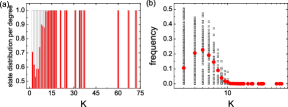
Figure 5: (a) Distributions of states in BA network. Cooperators are denoted by red bars, while defectors by white bars, the lengthes of which are proportional to the relative percentage of the respective state for each degree $k$. (b) Each agent’s frequency of state updating (open square) during the evolution of the system from the initial random state to the final equilibrium state within $25000$ generations. And the averages over agents with the same degree (dot). The simulation takes place on the BA network of size $N=1000$ and $m=2$, with interest rate $r=1.6$, strategy $\alpha=0$, which result in the frequency of cooperators $\rho_{C}=0.684$.

Similar to the former studies of other games Santos2005 ; Santos20061 ; Santos20062 , the heterogeneity intrinsic to SF NoCs also contributes to the enhancement of cooperation, by favoring cooperators to occupy the large degree agents so as to outperform defectors. The detailed description of the occupation of vertices with given degree is shown in Fig. 5(a). One can clearly find that, almost all hubs are occupied by cooperators, whereas defectors present merely at low degree vertices. In Fig. 5(b), we plot the state updating frequency of each agent during the evolution of the system from the initial state to the final equilibrium state. From the figures, we know that with respect to the small degree agents, the hubs always behave as cooperator and rarely change. During the evolution, when a hub is a defector investor, it can exploit and may easily invade most of its cooperator neighbors. However, in doing so, the number of neighbor cooperators will decrease in subsequent rounds, which in turn acts to reduce the total returns of such defector hub. Whenever its return becomes comparable to that of a cooperator neighbor, invasion may occur. On the contrary, however, once cooperators invade hubs, they will tend to increase the fraction of cooperator neighbors, in turn maximizing their own returns. In other words, once invading a hub, a cooperator becomes so successful that it is very difficult for defectors to ‘trike back’, as evidenced by the results shown in Fig. 5.

V conclusion

In summary, considering the heterogeneity of real-world NoCs, we have proposed an extended public goods interaction model in this paper. The investor bounded to the underlying network will distribute capital to pools proportionally to their attractiveness, which reflects the heterogeneous influence of pools on investors, with the investment strategy $\alpha$ regulating the value of attractiveness. From the comparative studies of the game dynamics upon square lattice and BA scale-free network, we found that heterogeneous structured population partially resolves the dilemma and improves social welfare. On one hand, the hub cooperators always remain stable, and spread cooperation to a larger fraction of the agents. On the other hand, cooperator investors can pay themselves off with more profit when taking small $\alpha$ investment strategy, which relaxes the social dilemma further and enhances the reproductive success of cooperation.

In addition, the qualitative features of the game dynamics sustain when the network size $N$ and the parameter $m$ of BA networks are different. The networks with smaller $m$ are proved to favor cooperation more, which can be attributed to the corresponding smaller group size Hauert ; Hauert4 .

We thank Dr. Xin-Jian Xu for helpful discussion. This work was supported by the Fundamental Research Fund for Physics and Mathematics of Lanzhou University under Grant No. Lzu05008.

References

- (1) J. von Neumann, and O. Morgenstern, Theory of Games and Economic Behaviour (Princeton University Press, Princeton, 1944).
- (2) J. Maynard Smith, and E. Szathmáry, The Major Transitions in Evolution (W. H. Freeman & Co., Oxford, 1995).
- (3) C. Hauert, S. De Monte, J. Hofbauer, and K. Sigmund, Science 296, 1129 (2002).
- (4) R.L. Trivers, Q. Rev. Biol. 46, 35 (1971).
- (5) R. Axelrod, and W.D. Hamilton, Science 211, 1390 (1981).
- (6) R.D. Alexander, The biology of moral systems (New York, NY: Aldine DE Gruyter, 1987).
- (7) M.A. Nowak, and K. Sigmund, Nature 393, 573 (1998).
- (8) M.A. Nowak, and K. Sigmund, Nature 437, 1291 (2005).
- (9) T.H. Clutton-Brock, and G.A. Parker, Nature 373, 209 (1995).
- (10) E. Fehr, and S. Gächter, Nature 415, 137 (2002).
- (11) M.A. Nowak, and R.M. May, Nature (London) 359, 826 (1992).
- (12) G. Szabó, and C. Tőke, Phys. Rev. E 58, 69 (1998).
- (13) C. Hauert, and M. Doebeli, Nature (London) 428, 643 (2004).
- (14) G. Szabó, and C. Hauert, Phys. Rev. Lett 89, 118101 (2002); G. Szabó, and C. Hauert, Phys. Rev. E 66, 062903 (2002); G. Szabó, and J. Vukov, Phys. Rev. E 69, 036107 (2004).
- (15) Z.-X. Wu, X.-J. Xu, Y. Chen, and Y.-H. Wang, Phys. Rev. E 71, 037103 (2005).
- (16) C. Hauert, S. De Monte, J. Hofbauer, and K. Sigmund, J. Theor. Biol. 218, 187 (2002).
- (17) J.H. Kagel, and A.E. Roth (eds.) The handbook of experimental economics (Princeton, NJ: Princeton University Press, 1995).
- (18) C. Hauert, and G. Szabó, Complexity 8, 31 (2003).
- (19) H. Brandt, C. Hauert, and K. Sigmund, Proc. Natl. Acad. Sci. 103, 495 (2006).
- (20) C. Hauert, M. Holmes, and M. Doebeli, Proc. R. Soc. B 273, 2565 (2006).
- (21) S.N. Dorogotsev, and J.F.F. Mendes, Evolution of Networks: From Biological Nets to the Internet and WWW (Oxford University, Oxford, 2003).
- (22) A.-L. Barabási, and R. Albert, Science 286, 509 (1999).
- (23) R. Albert, and A.-L. Barabási, Rev. Mod. Phys. 74, 47 (2002).
- (24) S. Boccaletti, V. Latora, Y. Moreno, M. Chavez, and D.-U. Hwang, Phys. Rep. 424, 175 (2006).
- (25) R.M. May, S. Gupta, and A.R. McLean, Phil. Trans. R. Soc. B 356, 901 (2001).
- (26) In the real financial system, investors always take a range of securities to invest. This is because if any particular security proves to be a bad investment, the impact on such a diversified portfolio is not as significant as having put all eggs in one basket.
- (27) Z.-X. Wu, X.-J. Xu, and Y.-H. Wang, Chin. Phys. Lett. 23, 531 (2005).
- (28) Z.-X. Wu, X.-J. Xu, Z.-G. Huang, S.-J. Wang, and Y.-H. Wang, Phys. Rev. E 74, 021107 (2005).
- (29) J.-Y. Guan, Z.-X. Wu, Z.-G. Huang, X.-J. Xu, and Y.-H. Wang, Europhys. Lett. 76, 1214 (2006).
- (30) From Eq. (9), we know that, for given agent , would be larger when is small, because the value of the larger which is small will have more contribution to .
- (31) F.C. Santos, and J.M. Pacheco, Phys. Rev. Lett. 95, 098104 (2005).
- (32) F.C. Santos, J.F. Rodrigues, and J.M. Pacheco, Proc. R. Soc. B 273, 51 (2006).
- (33) F.C. Santos, J.M. Pacheco, and T. Lenaerts, Proc. Natl. Acad. Sci. U.S.A. 103, 3490 (2006).