Theory of induced quadrupolar order in tetragonal YbRu₂Ge₂

Abstract

The tetragonal compound YbRu₂Ge₂ exhibits a non-magnetic transition at $T_{0}$=10.2K and a magnetic transition at $T_{1}$=6.5K in zero magnetic field. We present a model for this material based on a quasi-quartet of Yb³⁺ crystalline electric field (CEF) states and discuss its mean field solution. Taking into account the broadening of the specific heat jump at $T_{0}$ for magnetic field perpendicular to [001] and the decrease of $T_{0}$ with magnetic field parallel to [001], it is shown that ferro-quadrupole order of either O${}_{2}^{2}$ or O_xy - type are prime candidates for the non-magnetic transition. Considering the matrix element of these quadrupole moments, we show that the lower CEF states of the level scheme consist of a $\Gamma_{6}$ and a $\Gamma_{7}$ doublet. This leads to induced type of O${}_{2}^{2}$ and O_xy quadrupolar order parameters. The quadrupolar order introduces exchange anisotropy for planar magnetic moments. This causes a spin flop transition at low fields perpendicular [001] which explains the observed metamagnetism. We also obtain a good explanation for the temperature dependence of magnetic susceptibility and specific heat for fields both parallel and perpendicular to the [001] direction.

I Introduction

It is well known that some $f$-electron systems show multipole ordering. The phenomenon has attracted much attention, since features of multipole order are quite different from usual magnetic order. As a typical case, CeB₆ shows a kind of antiferro-quadrupole ordering at 3.4K, whose transition temperature increases with increasing magnetic fieldFujita ; Takigawa ; Effantin . For transition in NpO₂, an octupole ordering is proposed due to experimental results of resonant x-ray scattering Mannix ; Paixao ; Lovesey and NMR Tokunaga although a cusp at the transition temperature is observed in uniform susceptibilityRoss ; Erdos . There are at least two common properties between these compounds. At first, these compounds have cubic crystal structure. Secondly, the crystalline electric field (CEF) ground states of corresponding level schemes are quartet states, which are available only in cubic systems. It is thought that the quartet state is responsible for multipole ordering.

Recently, some anomalous properties have been observed in the tetragonal metallic compound YbRu₂Ge₂Jeevan . In specific heat measurement without magnetic field, there are three transition temperatures at $T_{0}$=10.2K, $T_{1}$=6.5K, and $T_{2}$=5.7K. It is important that the entropy around $T_{0}$ obtained by integration of specific heat data is very close to Rln4, which means the existence of a quasi-quartet state even in the tetragonal system. Applying a magnetic field perpendicular to [001] direction, the specific heat jump at $T_{0}$ broadens, and the peak position corresponding to $T_{0}$ seems to increase, while $T_{1}$ and $T_{2}$ merge and decrease. Increasing magnetic field further above 7T, no anomaly is found. On the other hand, in magnetic field parallel to [001], not only $T_{1}$ and $T_{2}$ but also $T_{0}$ decrease with increasing magnetic field. For the magnetic susceptibility $\chi_{\rm ab}$ in magnetic field perpendicular to [001], no anomaly appears at $T_{0}$, while a cusp is observed at $T_{1}$ for small magnetic fields. Furthermore, a metamagnetic transition at higher fields around 2T is regarded as spin-flop transition. The magnetic susceptibility $\chi_{\rm c}$ in field parallel to [001] is almost temperature independent between $T_{0}$ and $T_{1}$, and shows flat temperature dependence below $T_{1}$ after a slight decrease just below $T_{1}$. Because the value of the paramagnetic effective moment 4.5$\mu_{\rm B}$ is very close to magnetic moment of free Yb³⁺, it is a reasonable assumption that $f$-hole of Yb³⁺ is almost localized. Considering the quasi-quartet state in a localized picture, some multipole moments will be active at each site in the system. From these experimental data, it has been suggested that $T_{0}$ is a kind of quadrupole transition, while the phase below $T_{1}$ is regarded as antiferromagnetic phase with planar staggered momentJeevan . According to Jeevan ${\it et}$ ${\it al.}$, a change in magnetic structure may happen at $T_{2}$. We will ignore this subtlety in the following and consider only $T_{1}$.

In the theoretical analysis of CeB₆, Shiina ${\it et}$ ${\it al.}$ have provided a mean-field approximation for the effective Hamiltonian of localized $f$-electrons belonging to $\Gamma_{8}$ irreducible representation in O_h point group. In this case all multipole moments up to octupole are active Shiina . The relevant multipoles have been classified according to irreducible representations of the point group in zero magnetic field. Taking into account that some symmetry operations of O_h point group elements are lost in a magnetic field, the multipoles have been reclassified according to irreducible representations of the relevant point group in the magnetic field. Using these multipoles a mean-field approximation has been applied to an effective Hamiltonian to construct the $H$-$T$ phase diagram. After introduction of anisotropic interaction of quadrupoles, they have obtained a consistent explanation for the anomalous ordering in CeB₆. It should be noted that this approach is promising for multipole ordering not only in CeB₆ but also in TmTeTmTe , where Tm²⁺ has the same (4f)¹³ electronic configuration as Yb³⁺, and NpO₂Kubo .

In the present work, we apply this approach to investigate the phases of YbRu₂Ge₂. In this system, there are some significant differences to CeB₆, though a kind of quadrupole ordering is expected. At first, the crystal structure of YbRu₂Ge₂ is tetragonal, with point group D_4h. Second, noting that composition of the quasi-quartet depends on crystalline electric field parameters, it is expected that multipole ordering is also affected by the level scheme, while only the size of coupling constants decides on the favorable multipole ordering in cubic systemsShiina . Third, considering the present system is tetragonal, some multipoles are described only by induced moments, whose expectation value in the CEF ground state vanishes Trammell ; Bleaney . Especially, the second and third points bring additional complexity to identify a multipole transition. In order to explain the behavior of YbRu₂Ge₂, we introduce an effective Hamiltonian in the next section. Then, we apply a mean-field approximation for the Hamiltonian to identify the non-magnetic ordering state below $T_{0}$. Furthermore, we try to reproduce temperature dependences of specific heat and uniform susceptibility in magnetic field with anisotropic magnetic interaction. Finally, we summarize our results.

II Effective Hamiltonian

From analysis of uniform susceptibility, effective moment is estimated as 4.5$\mu_{\rm B}$, which is quite close to the value 4.54$\mu_{\rm B}$ for free Yb³⁺ ions. This means that the picture of localized hole in the 4$f$-shell will be reasonable for YbRu₂Ge₂. First we need to construct CEF level scheme of Yb³⁺, to extract relevant multipole moments, and then we introduce effective intersite interactions between the multipole moments.

II.1 CEF term

The total angular momentum $j$ of Yb³⁺-ion is $j=7/2$. The multiplet splits into four Kramers-doublets in tetragonal crystal structure of YbRu₂Ge₂. In tetragonal point group D_4h, $j=7/2$ multiplet is classified according to two-$\Gamma_{6}$ and two-$\Gamma_{7}$ irreducible representations. For two doublets belonging to the same $\Gamma$-irreducible representation, we call the lower and higher ones $\Gamma^{(1)}$ and $\Gamma^{(2)}$, respectively, in the following. These states are described by linear combination of free ion states $|\mu\rangle$=$|j\mu\rangle$ ($|\mu|\leq\frac{7}{2}$) as follows,

$$|\tau=1,\pm\rangle=|\Gamma_{6}^{(1)}\pm\rangle=\alpha_{11}|\frac{\pm 7}{2}\rangle+\alpha_{12}|\frac{\mp 1}{2}\rangle,$$ (1)

$$|\tau=2,\pm\rangle=|\Gamma_{6}^{(2)}\pm\rangle=\alpha_{21}|\frac{\pm 7}{2}\rangle+\alpha_{22}|\frac{\mp 1}{2}\rangle,$$ (2)

$$|\tau=3,\pm\rangle=|\Gamma_{7}^{(1)}\pm\rangle=\beta_{11}|\frac{\mp 5}{2}\rangle+\beta_{12}|\frac{\pm 3}{2}\rangle,$$ (3)

$$|\tau=4,\pm\rangle=|\Gamma_{7}^{(2)}\pm\rangle=\beta_{21}|\frac{\mp 5}{2}\rangle+\beta_{22}|\frac{\pm 3}{2}\rangle,$$ (4)

where $\mu$ is z-component of total angular momentum and + ($-$) of left-hand side shows pseudo-spin up (down) in Kramers-doublets.

Usually, CEF parameters are estimated by fitting calculated uniform susceptibility to the observed one. In addition, the inelastic neutron scattering (INS) gives important informations like splitting energy between the ground and first excited states in the level scheme. In recent INS experiment in YbRu₂Ge₂, the level scheme is reported with the splitting energy of 0.9 meVGeibel1 . Using the splitting energy, we have carried out the fitting of uniform susceptibility. Unfortunately, we could not obtain unique CEF level scheme from this procedure. However, from reasonable CEF level schemes, we obtain the following common features: (1) The splitting energy between the ground and first excited states is about 12K, which is estimated by reproducing the entropy obtained from specific heat data; (2) the ground and first excited states consist of one $\Gamma_{6}$ and one $\Gamma_{7}$ states, neither two $\Gamma_{6}$ nor two $\Gamma_{7}$ states; and (3) energy splittings of the second excited state from the ground state are at least thirty times larger than the observed transition temperature $T_{0}$=10.2K and the splitting energy between the ground and first excited states. Due to the third point, we can neglect upper two doublets, if we consider only low temperature region. The relevant CEF Hamiltonian is then given by

$$H_{\rm CEF}=-\sum_{{\bf i},\eta}\frac{\Delta_{0}}{2}(f_{{\bf i}6\eta}^{\dagger}f_{{\bf i}6\eta}-f_{{\bf i}7\eta}^{\dagger}f_{{\bf i}7\eta}),$$ (5)

where $\Delta_{0}$ is splitting energy from $\Gamma_{6}^{(1)}$ state to $\Gamma_{7}^{(1)}$ state. Here, $f_{{\bf i}\tau\eta}^{\dagger}$ is creation operator of $f$-hole with pseudo-spin $\eta$ in $\Gamma_{\tau}^{(1)}$ Kramers-doublet at site ${\bf i}$. Although we assume that the lower two doublets consist of one $\Gamma_{6}$ and one $\Gamma_{7}$ states, this assumption will be justified during identification of non-magnetic ordered state in YbRu₂Ge₂.

II.2 Zeeman term

The Zeeman term due to the applied field h is given by

$$H_{\rm Z}=-g_{J}\mu_{\rm B}\sum_{\bf i}{\bf h}\cdot{\bf J}_{\bf i},$$ (6)

where ${\bf J}$, $g_{J}$, and $\mu_{\rm B}$ are total angular momentum, Land$\acute{\rm e}$ $g$-factor of Yb³⁺, and Bohr magneton, respectively. With use of second quantization, x- and z-components of the angular momentum in $\Gamma_{6}$-$\Gamma_{7}$ subspace are expressed as

$$J^{\rm z}=c^{\rm z}_{66}S^{\rm z}_{66}+c^{\rm z}_{77}S^{\rm z}_{77},$$ (7)

$$J^{\rm x}=c^{\rm x}_{66}S^{\rm x}_{66}+c^{\rm x}_{77}S^{\rm x}_{77}+c^{\rm x}_{67}\frac{1}{\sqrt{2}}(S^{\rm x}_{67}+S^{\rm x}_{76}),$$ (8)

with $\alpha$-component of pseudo-spin operator given by

$$S^{\alpha}_{\tau\tau^{\prime}}=\frac{1}{2}\sum_{\eta,\eta^{\prime}}f_{\tau\eta}^{\dagger}\sigma^{\alpha}_{\eta\eta^{\prime}}f_{\tau^{\prime}\eta^{\prime}},$$ (9)

where ${\bf\sigma}^{\alpha}$ is $\alpha$-component of Pauli matrix. The coefficients $c^{\alpha}_{\tau\tau^{\prime}}$ are expressed by $\alpha_{12}$ and $\beta_{12}$ as

$$c^{\rm z}_{66}=7-8\alpha_{12}^{2},\hskip 14.22636ptc^{\rm z}_{77}=-5+8\beta_{12}^{2},$$ (10)

$$c^{\rm x}_{66}=4\alpha_{12}^{2},\hskip 14.22636ptc^{\rm x}_{77}=4\sqrt{3}\beta_{12}\sqrt{1-\beta_{12}^{2}},$$

$$c^{\rm x}_{67}=\sqrt{7}\sqrt{(1-\alpha_{12}^{2})(1-\beta_{12}^{2})}+\sqrt{30}\alpha_{12}\beta_{12}.$$ (11)

Therefore the coefficients $\alpha_{12}$ and $\beta_{12}$ which determine the structure of $\Gamma_{6}^{(1)}$ and $\Gamma_{7}^{(1)}$ states are incorporated through anisotropic effective $g$-factors in Eqs. (7,8). We comment on the limiting case of $\alpha_{12}=\beta_{12}=1$, which are very close to values estimated by fitting of uniform susceptibility in III. B.. As we have mentioned above, we consider only quasi-quartet consisting of one $\Gamma_{6}$ and one $\Gamma_{7}$ doublet at each site. As far as the quasi-quartet is concerned, multipole moments up to octupole are relevant as given in Table I. In this sense, the inter-site term will be always mapped to $j$=3/2 quartet system. In particular, with $\alpha_{12}=\beta_{12}=1$, the two Kramers doublets reduce to $|\pm\frac{1}{2}\rangle$ and $|\pm\frac{3}{2}\rangle$, which are belonging to $\Gamma_{6}$ and $\Gamma_{7}$ irreducible representations in D_4h point group. In addition the operator $J^{\rm z}$ in $j$=3/2 quartet system is the same as the operator given in Eq. (7) with $\alpha_{12}=\beta_{12}=1$. Therefore, when a magnetic field is applied in [001] direction, the present system with $\alpha_{12}=\beta_{12}=1$ is mapped to $j$=3/2 quartet system. However, such mapping is not applicable in magnetic field perpendicular along [001], due to differences of matrix elements of $J^{\rm x}$ and $J^{\rm y}$ between $j$=3/2 quartet system and the present system with $\alpha_{12}=\beta_{12}=1$.

II.3 Inter-site term

In the present case, we consider that $f$-hole localizes at each Yb-site. From the simplification mentioned above, we have one $\Gamma_{6}$ doublet and one $\Gamma_{7}$ doublet. Even in the simplification, there are 15 kinds of multipoles at each Yb-site. In order to describe the multipoles, we introduce bases of multipoles $\phi^{\Gamma}_{n}$ belonging to $\Gamma$-irreducible representation in D_4h point group. In Table. 1, we classify $\phi^{\Gamma}_{n}$ according to irreducible representations in D_4h point group, where in addition to $S^{\alpha}_{\tau\tau^{\prime}}$, we use a $f$-charge operator

$$\rho_{\tau\tau^{\prime}}=\frac{1}{2}\sum_{\eta}f_{\tau\eta}^{\dagger}f_{\tau^{\prime}\eta}.$$ (12)

Since classification of multipoles up to octupole is also shown in Table. 1, correspondence between multipole and $\phi^{\Gamma}_{n}$ will be clear. For example, the x-component of dipole moment $J^{\rm x}$ is described by a linear combination of $\phi^{\Gamma_{5}^{-}}_{nx}$, which is consistent with Eq.(8).

Now, considering that metallic behavior has been observed in YbRu₂Ge₂, effective RKKY interactions between the multipoles are present, which are derived through the Schrieffer-Wolff transformation from hybridization term between 4$f$- and conduction-electrons. Noting that the Yb-sites in the compound form body-centered tetragonal lattice, inter-layer interactions should favor ferro-type order, since antiferro-couplings would lead to frustration. In the following, we consider multipole ordering within a mean-field theory for Yb in the body centered tetragonal structure, assuming that the ordering takes place either at the zone center $\tilde{\bf q}=0$ (ferro) or at the zone boundary $\tilde{\bf q}$=($\pi$,$\pi$,0) (antiferro). If we consider only diagonal term of nearest-neighbour couplings, the inter-site term of Hamiltonian $H_{\rm int}$ is given by

$$H_{\rm int} = -\sum_{{\bf i}\neq{\bf j}}\sum_{\Gamma,n}J^{\Gamma}_{{\bf i}-{\bf j}n}\phi^{\Gamma}_{{\bf i}n}\phi^{\Gamma}_{{\bf j}n},$$ (13)

$$= -\frac{1}{N_{0}}\sum_{\Gamma,n}\sum_{\bf q}J^{\Gamma}_{n}({\bf q})\phi^{\Gamma}_{n}({\bf-q})\phi^{\Gamma}_{n}({\bf q}),$$ (14)

with $\phi^{\Gamma}_{n}({\bf q})=\sum_{\bf i}e^{-{\rm i}{\bf q}\dot{\bf i}}\phi^{\Gamma}_{{\bf i}n}$, where $J^{\Gamma}_{n}$ is a coupling constant between $\phi^{\Gamma}_{n}$, and $N_{0}$ is the number of Yb-sites in crystal. In Eq. (14), $J^{\Gamma}_{n}({\bf q})$ and $\phi^{\Gamma}_{n}({\bf q})$ are Fourier components of coupling constants and $\phi^{\Gamma}_{{\bf i}n}$, respectively. For square lattice, $J^{\Gamma}_{n}({\bf q})$ is given by

$$J^{\Gamma}_{n}({\bf q})=2J^{\Gamma}_{n}(\cos{q_{x}}+\cos{q_{y}}).$$ (15)

II.4 Resulting effective Hamiltonian

In order to explain low temperature property of YbRu₂Ge₂, effective Hamiltonian used in the following is described by

$$H_{\rm eff}=H_{\rm CEF}+H_{\rm Z}+H_{\rm int}.$$ (16)

As we have already mentioned, we can determine $|\Delta_{0}|$ from the entropy. However, in Zeeman term $H_{\rm Z}$, there are two free parameters, which control the weight of $|\pm 1/2\rangle$ and $|\pm 3/2\rangle$ in $\Gamma_{6}^{(1)}$ and $\Gamma_{7}^{(1)}$ states, respectively. In addition, we have coupling constants $J^{\Gamma}_{n}$, which will be estimated in the following sections. Then we apply a mean-field approximation for the effective Hamiltonian to calculate thermodynamic quantities and the phase diagrams.

Table 1: Classification of multipoles and relevant bases of the multipoles $\phi^{\Gamma}_{n}$ according to irreducible representations of D_4h point group. The first column shows irreducible representation of D_4h. The second and third ones describe multipoles and $\phi^{\Gamma}_{n}$ belonging to $\Gamma$ irreducible representation, respectively. Here $J$, $O$, and $T$ in the second column are dipole, quadrupole, and octupole moments, respectively. The fourth column shows expression of corresponding local susceptibility of $\phi^{\Gamma}_{n}$ with splitting energy $\Delta$ from $\Gamma_{6}$ to $\Gamma_{7}$ states. The superscript $\pm$ of irreducible representation expresses the parity with respect to time reversal.

$\Gamma$ (D4h)	multipole	$\phi^{\Gamma}_{n}$	$\chi^{{\rm L}\Gamma}_{nn}$
$\Gamma_{1}^{+}$	$O_{2}^{0}$	$\phi^{\Gamma_{1}^{+}}$= $\frac{1}{\sqrt{2}}(\rho_{66}-\rho_{77})$	$\frac{1}{8T}(1-\tanh^{2}{\frac{\Delta}{2T}})$
$\Gamma_{3}^{+}$	$O_{2}^{2}$	$\phi^{\Gamma_{3}^{+}}$= $\frac{1}{\sqrt{2}}(\rho_{67}+\rho_{76})$	$\frac{1}{4\Delta}\tanh{\frac{\Delta}{2T}}$
$\Gamma_{4}^{+}$	$O_{xy}$	$\phi^{\Gamma_{4}^{+}}$= $\frac{\rm i}{\sqrt{2}}(S^{\rm z}_{67}-S^{\rm z}_{76})$	$\frac{1}{4\Delta}\tanh{\frac{\Delta}{2T}}$
$\Gamma_{5}^{+}$	$O_{yz}$	$\phi^{\Gamma_{5}^{+}}_{x}$= $\frac{\rm i}{\sqrt{2}}(S^{\rm x}_{67}-S^{\rm x}_{76})$	$\frac{1}{4\Delta}\tanh{\frac{\Delta}{2T}}$
	$O_{zx}$	$\phi^{\Gamma_{5}^{+}}_{y}$= $\frac{\rm i}{\sqrt{2}}(S^{\rm y}_{67}-S^{\rm y}_{76})$	$\frac{1}{4\Delta}\tanh{\frac{\Delta}{2T}}$
$\Gamma_{2}^{-}$	$J^{\rm z}$	$\phi^{\Gamma_{2}^{-}}_{1}$=$S^{\rm z}_{66}$	$\frac{1}{8T}(1+\tanh{\frac{\Delta}{2T}})$
	$T_{\rm z}^{\alpha}$	$\phi^{\Gamma_{2}^{-}}_{2}$=$S^{\rm z}_{77}$	$\frac{1}{8T}(1-\tanh{\frac{\Delta}{2T}})$
$\Gamma_{3}^{-}$	$T_{xyz}$	$\phi^{\Gamma_{3}^{-}}$= $\frac{\rm i}{\sqrt{2}}(\rho_{67}-\rho_{76})$	$\frac{1}{4\Delta}\tanh{\frac{\Delta}{2T}}$
$\Gamma_{4}^{-}$	$T_{\rm z}^{\beta}$	$\phi^{\Gamma_{4}^{-}}$= $\frac{1}{\sqrt{2}}(S^{\rm z}_{67}+S^{\rm z}_{76})$	$\frac{1}{4\Delta}\tanh{\frac{\Delta}{2T}}$
$\Gamma_{5}^{-}$	$J^{\rm x}$	$\phi^{\Gamma_{5}^{-}}_{1x}$=$S^{\rm x}_{66}$	$\frac{1}{8T}(1+\tanh{\frac{\Delta}{2T}})$
	$T_{\rm x}^{\alpha}$	$\phi^{\Gamma_{5}^{-}}_{2x}$=$S^{\rm x}_{77}$	$\frac{1}{8T}(1-\tanh{\frac{\Delta}{2T}})$
	$T_{\rm x}^{\beta}$	$\phi^{\Gamma_{5}^{-}}_{3x}$= $\frac{1}{\sqrt{2}}(S^{\rm x}_{67}+S^{\rm x}_{76})$	$\frac{1}{4\Delta}\tanh{\frac{\Delta}{2T}}$
	$J^{\rm y}$	$\phi^{\Gamma_{5}^{-}}_{1y}$=$S^{\rm y}_{66}$	$\frac{1}{8T}(1+\tanh{\frac{\Delta}{2T}})$
	$T_{\rm y}^{\alpha}$	$\phi^{\Gamma_{5}^{-}}_{2y}$=$S^{\rm y}_{77}$	$\frac{1}{8T}(1-\tanh{\frac{\Delta}{2T}})$
	$T_{\rm y}^{\beta}$	$\phi^{\Gamma_{5}^{-}}_{3y}$= $\frac{1}{\sqrt{2}}(S^{\rm y}_{67}+S^{\rm y}_{76})$	$\frac{1}{4\Delta}\tanh{\frac{\Delta}{2T}}$

III Analysis of Transition at $T_{0}$

In this section, we develop a mean-field theory for the effective Hamiltonian to analyze non-magnetic transition at $T_{0}$. After comparing phase diagrams for all types of ferro- and antiferro-quadrupole ordering with experimental one, we propose a prefered type of quadrupole order in YbRu₂Ge₂.

III.1 Mean-field approximation for quadrupolar order

At first, we give mean-field Hamiltonian to determine transition line in $H$-$T$ phase diagram. We assume that multipole ordered state is specified by irreducible representation $\Gamma$ and ordering wave vector $\tilde{\bf q}$. From the effective model, we obtain easily the mean-field Hamiltonian

$$H_{\rm MF}=H_{\rm CEF}+H_{\rm Z}+\tilde{H}_{\rm int},$$ (17)

$$\tilde{H}_{\rm int}=-\frac{1}{N_{0}}\sum_{\Gamma,n}\sum_{\bf q}J^{\Gamma}_{n}({\bf q})(2\langle\phi^{\Gamma}_{n}({\bf q})\rangle\phi^{\Gamma}_{n}({\bf q})$$

$$\hskip 116.6563pt-\langle\phi^{\Gamma}_{n}({\bf q})\rangle^{2}),$$ (18)

with

$$\langle\cdots\rangle=\frac{{\rm Tr}\hskip 2.84526pte^{-H_{\rm MF}/T}\cdots}{{\rm Tr}\hskip 2.84526pte^{-H_{\rm MF}/T}}$$ (19)

where $T$ is the temperature.

We consider three cases, (1) system in zero magnetic field, (2) system in magnetic field parallel to [001] direction, and (3) system in magnetic field parallel to [100] direction, whose point groups are D_4h, C_4v, and C_2v, respectively. In Table 2 and 3, bases of multipoles are classified according to irreducible representations of C_4v and C_2v point group, respectively. In order to develop a general formalism, we call bases of multipoles belonging to $\Gamma$-irreducible representation generically $\psi^{\Gamma}_{n}$ in any point group G (D_4h, C_4v, and C_2v). For D_4h point group, $\psi^{\Gamma}_{n}$ is equivalent to $\phi^{\Gamma}_{n}$ given in Table. 1 . For non-zero field the corresponding lower symmetry point groups C_4v, and C_2v have basis functions $\psi^{\Gamma}_{n}$ that may still be directly expressed in terms of the D_4h basis functions $\phi^{\Gamma}_{n}$ as shown in Tables II and III. In the following, we discuss only disordered, ferro-, and antiferro-ordered states, which is reasonable since we restrict to nearest-neighbor interaction in $H_{\rm int}$. In the disordered state only the fully symmetric multipole $\psi^{\Gamma_{1}}_{n}$ (O${}_{2}^{0}$ in zero field) has a non-zero expectation value $\langle\psi^{\Gamma_{1}}_{n}({\bf 0})\rangle$. It leads to the background temperature dependence of $\Gamma_{6}-\Gamma_{7}$ splitting as shown later. In ferro-ordered state belonging to $\Gamma$-irreducible representation, $\langle\psi^{\Gamma}_{n}({\bf 0})\rangle$ have finite values in addition to $\langle\psi^{\Gamma_{1}}_{n}({\bf 0})\rangle$. In antiferro-ordered state belonging to $\Gamma$-irreducible representation, allowed expectation values are $\langle\psi^{\Gamma}_{n}(\tilde{\bf q})\rangle$ and $\langle\psi^{\Gamma_{1}}_{n}({\bf 0})\rangle$.

Table 2: Classification of $\phi^{\Gamma}_{n}$ according to irreducible representations of C_4v, which is point group of tetragonal system in magnetic field parallel to [001]. Here, we note that $\phi^{\Gamma}_{n}$ are bases of multipoles belonging to $\Gamma$ irreducible representation in D_4h point group. The first column shows irreducible representation of C_4v. The second, third, and fourth ones describe quadrupole, $\phi^{\Gamma^{+}}_{n}$, and $\phi^{\Gamma^{-}}_{n}$ belonging to each irreducible representation in C_4v, respectively.

$\Gamma$ (C4v)	$O$	$\phi^{\Gamma^{+}}_{n}$ (even)	$\phi^{\Gamma^{-}}_{n}$ (odd)
$\Gamma_{1}$	$O_{2}^{0}$	$\phi^{\Gamma_{1}^{+}}$= $\frac{1}{\sqrt{2}}(\rho_{66}-\rho_{77})$	$\phi^{\Gamma_{2}^{-}}_{1}$=$S^{\rm z}_{66}$
			$\phi^{\Gamma_{2}^{-}}_{2}$=$S^{\rm z}_{77}$
$\Gamma_{3}$	$O_{2}^{2}$	$\phi^{\Gamma_{3}^{+}}$= $\frac{1}{\sqrt{2}}(\rho_{67}+\rho_{76})$	$\phi^{\Gamma_{4}^{-}}$= $\frac{1}{\sqrt{2}}(S^{\rm z}_{67}+S^{\rm z}_{76})$
$\Gamma_{4}$	$O_{\rm xy}$	$\phi^{\Gamma_{4}^{+}}$= $\frac{\rm i}{\sqrt{2}}(S^{\rm z}_{67}-S^{\rm z}_{76})$	$\phi^{\Gamma_{3}^{-}}$= $\frac{\rm i}{\sqrt{2}}(\rho_{67}-\rho_{76})$
$\Gamma_{5}$	$O_{\rm yz}$	$\phi^{\Gamma_{5}^{+}}_{x}$= $\frac{\rm i}{\sqrt{2}}(S^{\rm x}_{67}-S^{\rm x}_{76})$	$\phi^{\Gamma_{5}^{-}}_{1y}$=$S^{\rm y}_{66}$
			$\phi^{\Gamma_{5}^{-}}_{2y}$=$S^{\rm y}_{77}$
			$\phi^{\Gamma_{5}^{-}}_{3y}$= $\frac{1}{\sqrt{2}}(S^{\rm y}_{67}+S^{\rm y}_{76})$
	$O_{\rm zx}$	$\phi^{\Gamma_{5}^{+}}_{y}$= $\frac{\rm i}{\sqrt{2}}(S^{\rm y}_{67}-S^{\rm y}_{76})$	$\phi^{\Gamma_{5}^{-}}_{1x}$=$S^{\rm x}_{66}$
			$\phi^{\Gamma_{5}^{-}}_{2x}$=$S^{\rm x}_{77}$
			$\phi^{\Gamma_{5}^{-}}_{3x}$= $\frac{1}{\sqrt{2}}(S^{\rm x}_{67}+S^{\rm x}_{76})$

Table 3: Classification of $\phi^{\Gamma}_{n}$ according to irreducible representations of C_2v, which is point group of tetragonal system in magnetic field parallel to [100]. Here, we note that $\phi^{\Gamma}_{n}$ are bases of multipoles belonging to $\Gamma$ irreducible representation in D_4h point group. The first column shows irreducible representation of C_2v. The second, third, and fourth ones describe quadrupole, $\phi^{\Gamma^{+}}_{n}$, and $\phi^{\Gamma^{-}}_{n}$ belonging to each irreducible representation in C_2v, respectively.

$\Gamma$ (C2v)	$O$	$\phi^{\Gamma^{+}}_{n}$ (even)	$\phi^{\Gamma^{-}}_{n}$ (odd)
$\Gamma_{1}$	$O_{2}^{0}$	$\phi^{\Gamma_{1}^{+}}$= $\frac{1}{\sqrt{2}}(\rho_{66}-\rho_{77})$	$\phi^{\Gamma_{5}^{-}}_{1x}$=$S^{\rm x}_{66}$
	$O_{2}^{2}$	$\phi^{\Gamma_{3}^{+}}$= $\frac{1}{\sqrt{2}}(\rho_{67}+\rho_{76})$	$\phi^{\Gamma_{5}^{-}}_{2x}$=$S^{\rm x}_{77}$
			$\phi^{\Gamma_{5}^{-}}_{3x}$= $\frac{1}{\sqrt{2}}(S^{\rm x}_{67}+S^{\rm x}_{76})$
$\Gamma_{2}$	$O_{\rm yz}$	$\phi^{\Gamma_{5}^{+}}_{x}$= $\frac{\rm i}{\sqrt{2}}(S^{\rm x}_{67}-S^{\rm x}_{76})$	$\phi^{\Gamma_{3}^{-}}$= $\frac{\rm i}{\sqrt{2}}(\rho_{67}-\rho_{76})$
$\Gamma_{3}$	$O_{\rm xy}$	$\phi^{\Gamma_{4}^{+}}$= $\frac{\rm i}{\sqrt{2}}(S^{\rm z}_{67}-S^{\rm z}_{76})$	$\phi^{\Gamma_{5}^{-}}_{1y}$=$S^{\rm y}_{66}$
			$\phi^{\Gamma_{5}^{-}}_{2y}$=$S^{\rm y}_{77}$
			$\phi^{\Gamma_{5}^{-}}_{3y}$= $\frac{1}{\sqrt{2}}(S^{\rm y}_{67}+S^{\rm y}_{76})$
$\Gamma_{4}$	$O_{\rm zx}$	$\phi^{\Gamma_{5}^{+}}_{y}$= $\frac{\rm i}{\sqrt{2}}(S^{\rm y}_{67}-S^{\rm y}_{76})$	$\phi^{\Gamma_{2}^{-}}_{1}$=$S^{\rm z}_{66}$
			$\phi^{\Gamma_{2}^{-}}_{2}$=$S^{\rm z}_{77}$
			$\phi^{\Gamma_{4}^{-}}$= $\frac{1}{\sqrt{2}}(S^{\rm z}_{67}+S^{\rm z}_{76})$

For transition from disordered state to either ferro- or antiferro-multipole ordered state, we usually consider first- and second-order transitions. In a ferro- (or antiferro-) multipole ordered state belonging to $\Gamma$ irreducible representation in point group, expectation values of multipole moments $\langle\psi^{\Gamma}_{n}({\bf 0})\rangle$ (or $\langle\psi^{\Gamma}_{n}(\tilde{\bf q})\rangle$) have non-zero values. In general, free energy of ordered state is lower than that of disordered state below the transition temperature. The explicit expression of free energy in mean field approximation has already been given by Shiina et al. Shiina . In particular, if the transition is of second-order, all order parameters continuously reduce to zero on approaching the transition point. We use linearized mean-field equation to determine the second-order transition point, by expanding the partition function with respect to $\tilde{H}_{\rm int}$ given in Eq. (18). For transition to ordered state specified by irreducible representation $\Gamma$ of point group and ordering wave vector $\tilde{\bf q}$ it is given by

$$\langle\psi^{\Gamma}_{n}(\tilde{\bf q})\rangle=\sum_{m}\chi^{{\rm L}\Gamma}_{nm}2J^{\Gamma}_{m}(\tilde{\bf q})\langle\psi^{\Gamma}_{m}(\tilde{\bf q})\rangle.$$ (20)

with local susceptibility $\chi^{{\rm L}\Gamma}_{nn^{\prime}}$ defined by

$$\chi^{{\rm L}\Gamma}_{nn^{\prime}}=\int^{1/T}_{0}d\tau\hskip 2.84526pt\langle\psi^{\Gamma}_{{\bf i}n}(\tau)\psi^{\Gamma}_{{\bf i}n^{\prime}}\rangle-\delta_{\Gamma=\Gamma_{1}}\frac{\langle\psi^{\Gamma_{1}}_{{\bf i}n}\rangle\langle\psi^{\Gamma_{1}}_{{\bf i}n^{\prime}}\rangle}{T},$$ (21)

where $\tau$ is the imaginary time coordinate. The $\chi^{{\rm L}\Gamma}_{nn^{\prime}}$ are calculated in the limit of $\langle\psi^{\Gamma}_{n}(\tilde{\bf q})\rangle\rightarrow$ 0. The linearized mean-field equation has non-trivial solution only when the maximum eigenvalue of 2$\hat{\chi}^{{\rm L}\Gamma}J^{\Gamma}_{m}(\tilde{\bf q})$ becomes unity. We note that the transition becomes second-order, only if the transition point determined by linearized mean-field equation (20) is the same point where the free energies of the two states are equal.

III.2 Estimation of coupling constants

In our mean-field Hamiltonian, there are various parameters $\Delta_{0}$, $\alpha_{12}$, $\beta_{12}$ and $J^{\Gamma}_{n}$. At first, we consider disordered state in zero magnetic field. In this case, only allowed multipole is the uniform component of $\langle\phi^{\Gamma_{1}^{+}}\rangle$. Then, $\Delta_{0}$ is renormalized as

$$\Delta=\Delta_{0}+\frac{1}{2}J^{\Gamma_{1}^{+}}({\bf 0})\tanh{\frac{\Delta}{2T}}.$$ (22)

For estimation of $\Delta_{0}$ and $J^{\Gamma_{1}^{+}}({\bf 0})$=$4J^{\Gamma_{1}^{+}}$, we assume $\Delta(T=12K)=$12K and $\Delta_{0}=$8K, which gives $\Delta(T=T_{0}=10.2K)=$12.8K and $J^{\Gamma_{1}^{+}}=$4.3K. By choosing these parameter values, we obtain reasonable temperature dependence of entropy around $T_{0}$. In the following calculation, we fix these values of $\Delta_{0}$ and $J^{\Gamma_{1}^{+}}$.

Now we determine the values of $\alpha_{12}$ and $\beta_{12}$. These affect the magnetic anisotropy of the uniform susceptibility. Experimentally, the uniform susceptibility in magnetic field perpendicular to [001] is quite large compared to that in magnetic field parallel to [001]. The magnetic anisotropy is successfully reproduced by using the following lower two CEF states: The ground CEF state has almost pure $|\mp 1/2\rangle$ character belonging to $\Gamma_{6}$-irreducible representation, while the first-excited CEF state is almost pure $|\pm 3/2\rangle$ belonging to $\Gamma_{7}$-irreducible representation. Then the lower two CEF states are described by $\alpha_{12}\approx 1$ and $\beta_{12}\approx 1$, while $\alpha_{11}\approx\alpha_{22}\approx 0$ Geibel1 . With these values of $\alpha_{12}$ and $\beta_{12}$, contribution to $J^{\rm z}$ from the first excited $\Gamma_{7}$ state cancels out contribution from the ground $\Gamma_{6}$ state, while magnitude of $g$-factor $c_{66}^{\rm x}$ coming from the ground $\Gamma_{6}$ state in magnetic field parallel to [100] is four times larger than $c_{66}^{\rm z}$. Therefore, this CEF level scheme seems to be consistent with the observed magnetic anisotropy of the uniform susceptibility. In the following, we study transitions in the compound with these parameter values.

Furthermore, we have many interaction parameters in the inter-site term. Because the highest transition takes place at $T_{0}$, each multipole interaction has an upper limit. We estimate the upper limit of each coupling constant, by assuming that the transition to each ordered state takes place at $T_{0}$ in zero field. Since we use the linearized mean-field equation (20), we need to evaluate $\chi^{{\rm L}\Gamma}_{nn^{\prime}}$. In D_4h point group, the matrix $\hat{\chi}^{{\rm L}\Gamma}$ has diagonal form for each $\Gamma$. Each eigenvalue of $n$-th component in $\Gamma$ is given by

$$\lambda^{\Gamma}_{n}=2J^{\Gamma}_{n}(\tilde{\bf q})\chi^{{\rm L}\Gamma}_{nn}$$ (23)

where expressions for $\chi^{{\rm L}\Gamma}_{nn}$ are summarized in 4th column in Table. 1. Specifically, for each of the three two-dimensional representations, ($J^{\rm x}$, $J^{\rm y}$), ($T^{\alpha}_{\rm x}$, $T^{\alpha}_{\rm y}$), and ($T^{\beta}_{\rm x}$, $T^{\beta}_{\rm y}$) in Table I, we assume that the upper limit of coupling constant is independent on $n$. Together with one-dimensional representation, the upper limit of coupling constant for $\Gamma$ irreducible representation $J^{\Gamma}_{\rm c}(\tilde{\bf q})$ is then given by

$$2J^{\Gamma}_{\rm c}(\tilde{\bf q})=\frac{1}{{\rm max}\hskip 2.84526pt\chi^{{\rm L}\Gamma}_{nn}(T=T_{0})}.$$ (24)

In Table 4, by using the splitting energy $\Delta$ determined above, we list the calculated values of $1/8{\rm max}\hskip 2.84526pt\chi^{{\rm L}\Gamma}_{nn}(T=T_{0})$, which is equal to upper limit value of $J^{\Gamma}$ with factor 1/2$z$=1/8, where $z$ is the square lattice coordination number. If we use corresponding upper limit for every coupling constant, all transition temperatures to ordered states would become degenerate at $T_{0}$. In calculating the transition to an ordered state with a primary order parameter $\phi^{\Gamma}_{n}$, we assume that only the coupling constant for $\phi^{\Gamma}_{n}$ is at the upper limit. All others are reduced by a factor $\alpha_{\Gamma^{\prime}}$ ($\Gamma^{\prime}\neq\Gamma$)

$$J^{\Gamma}_{n}(\tilde{\bf q})=J^{\Gamma}_{\rm c}(\tilde{\bf q}),$$

$$J^{\Gamma^{\prime}}_{n}(\tilde{\bf q})=\alpha_{\Gamma^{\prime}}J^{\Gamma^{\prime}}_{\rm c}(\tilde{\bf q})\hskip 28.45274pt{\rm for}\hskip 5.69054pt\Gamma^{\prime}\neq\Gamma$$ (25)

where $0<\alpha_{\Gamma^{\prime}}<1$ is a ratio of actual coupling constant $J^{\Gamma}$ to the critical value $J^{\Gamma}_{\rm c}$. Present available experimental data do not allow a unique determination of coupling constants. Only that for the primary ferroquadrupole order parameter may be fixed by the transition temperature T₀. In order to obtain a low-field behaviour of $T_{0}(h)$ which is insensitive to the details of the model we assume $\alpha_{\Gamma^{\prime}}$=0.5 for the remaining coupling strengths.

Table 4: Coupling constants used for analysis of YbRu₂Ge₂. The first column shows irreducible representation of D_4h. The second column shows upper limits of magnitudes of coupling constants for having $\phi^{\Gamma}_{n}$ order parameter at T₀. The third column shows coupling constants used in the model calculation of Sec. V. Here plus/minus sign for $J^{\Gamma}$ denotes ferro-/antiferro coupling. The value in parentheses exhibits reduced coupling constant between $\phi^{\Gamma_{5}^{-}}_{3y}$.

$\Gamma$ (D4h)	1/8${\rm max}\hskip 2.84526pt\chi^{{\rm L}\Gamma}_{nn}(T=T_{0})$ [K]	$J^{\Gamma}$ [K]
$\Gamma_{1}^{+}$	14.8	4.3
$\Gamma_{3}^{+}$	11.5	11.5
$\Gamma_{4}^{+}$	11.5	-3.0
$\Gamma_{5}^{+}$	11.5	-3.0
$\Gamma_{2}^{-}$	6.6	1.7
$\Gamma_{3}^{-}$	11.5	-3.0
$\Gamma_{4}^{-}$	11.5	-3.0
$\Gamma_{5}^{-}$	6.6	-3.4 (-2.1)

III.3 Order parameter candidates for transition at $T_{0}$

Before we discuss candidates for transition at $T_{0}$, we note a property of lower two CEF states for magnetic field parallel to [001]. As we have mentioned in previous subsection, the ground CEF state belonging to $\Gamma_{6}$ is lower than the first-excited CEF state belonging to $\Gamma_{7}$ by 12.8K at $T_{0}$ in zero magnetic field. Since the magnetic field parallel to [001] does not break 4-fold symmetry, we still can distinguish the $\Gamma_{6}$ and $\Gamma_{7}$ states. In this case their energies are easily obtained as $-\frac{\Delta}{2}\mp g_{J}\mu_{\rm B}c^{\rm z}_{66}h$ for the $\Gamma_{6}$ Kramers doublet and $\frac{\Delta}{2}\mp g_{J}\mu_{\rm B}c^{\rm z}_{77}h$ for the $\Gamma_{7}$ state. There are two remarkable points in the present level scheme; (1) $c^{\rm z}_{66}$ has negative sign while $c^{\rm z}_{77}$ is positive, and (2) magnitude of $c^{\rm z}_{77}$ is three times larger than that of $c^{\rm z}_{66}$. From these facts we can expect a level crossing in the high field region of the disordered phase, where the CEF ground state changes from $\Gamma_{6}$ in low field to $\Gamma_{7}$ in high fieldcomment1 .

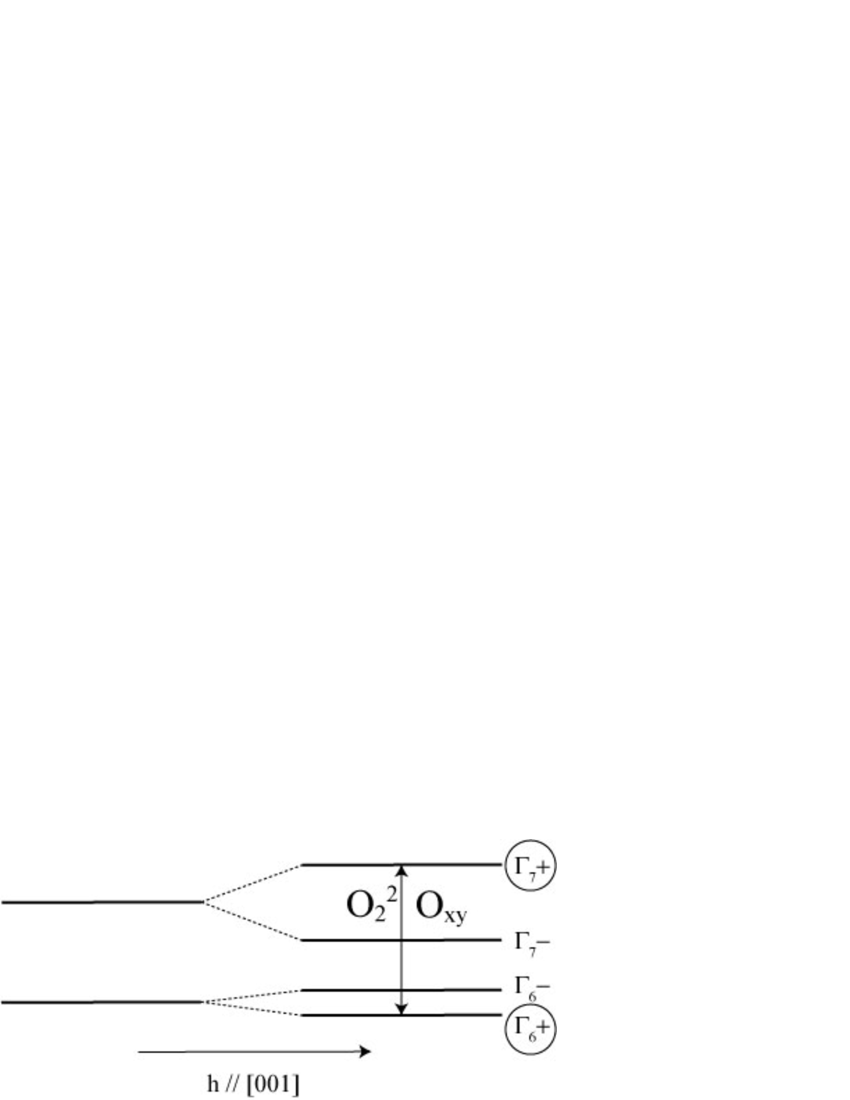
Figure 2: Schematic view of lower two CEF states in magnetic field parallel to [001]. By operators of $O_{2}^{2}$ and $O_{xy}$, which are equivalent to $\phi^{\Gamma_{3}^{+}}$=$\frac{1}{\sqrt{2}}(\rho_{67}+\rho_{76})$ and $\phi^{\Gamma_{4}^{+}}$= $\frac{\rm i}{\sqrt{2}}(S^{\rm z}_{67}-S^{\rm z}_{76})$, respectively, the ground $\Gamma_{6}$ state couples only with the highest $\Gamma_{7}$ state in low magnetic field region. This leads to the induced type quadrupole order below $T_{0}$. The energy difference between these two states increases with increasing magnetic field.

In the following we discuss the transition line of $T_{0}(h)$ in magnetic field parallel to [001]. From experimental result, the specific heat data shows that the transition temperature of the non-magnetic phase decreases with increasing magnetic field. As mentioned before, we assume that the non-magnetic transition is obtained by ordering of quadrupole moment. However, we do not know the character of the quadrupole moment among the possible $O_{2}^{0}$, $O_{2}^{2}$, $O_{xy}$, and ($O_{yz}$, $O_{zx}$) cases, and even whether the ordering is of ferro- or antiferro-type. In order to identify the type of quadrupole ordering, we calculate transition lines for all kinds of quadrupole orderings to compare with the experimental one. Firstly, since coupling constant between $O_{2}^{0}$ is ferro-like as estimated in the previous subsection, and ferro-component of $O_{2}^{0}$ is allowed even in the disordered state belonging to $\Gamma_{1}$ in C_4v point group (Table 2), we exclude any ordering of $O_{2}^{0}$ from candidates of the transition at $T_{0}$. It does not break any symmetry and hence cannot lead to a specific heat jump. Secondly, we show transition lines for other types of quadrupole orderings in Fig. 1, where for coupling constants other than the primary order parameter, $\alpha_{\Gamma^{\prime}}$=0.5 is chosen. Considering the behavior of experimental specific heat, ferro-$O_{2}^{2}$ and ferro-$O_{xy}$ orderings are consistent with the experiment among all types of quadrupole orderings. From calculated results we conclude that transition to ferro-$O_{2}^{2}$ (or ferro-$O_{xy}$) ordering state is of second-order in low magnetic field region. In order to explain a decrease of transition temperature in the magnetic field, we show schematic view of magnetic field dependence of level scheme with possible transitions for $O_{2}^{2}$ and $O_{xy}$ in Fig. 2. In both $O_{2}^{2}$ and $O_{xy}$ ordering states, the ground CEF state $|\Gamma_{6}+\rangle$ couples only with highest state $|\Gamma_{7}+\rangle$, therefore, $O_{2}^{2}$ and $O_{xy}$ order are of induced type because the quadrupole expectation value in the ground state vanishes. In addition, splitting energy between these states increases with increasing magnetic field. Then, since the energy denominator of the dominant term of corresponding local susceptibility Eq. (21) increases, the second-order transition temperature decreases with increasing magnetic field. On the other hand, for ordering of $O_{yz}$ or $O_{zx}$, transition temperature of these quadrupole orderings increases with increasing magnetic field, since splitting energy between the ground CEF state and excited state $|\Gamma_{7}-\rangle$ decreases.

We now consider behavior in magnetic field perpendicular to [001]. From specific heat experiment, it is shown that the anomaly of specific heat jump broadens with increasing magnetic field. This means that the transition at $T_{0}$ in zero magnetic field reduces to a crossover in magnetic field perpendicular to [001]. We note that crossover does not break any symmetry. Instead of transition temperature $T_{0}$, we define a characteristic temperature $T^{*}$ as an inflection point of the specific heat divided by temperature. Let us assume antiferro-quadrupole ordering, which breaks at least translational symmetry. Since this would cause a specific heat jump, we exclude antiferro-quadrupole ordered state from the scenario of crossover. On the other hand, ferro-quadrupole ordering in general breaks local rotational symmetry, although the translational symmetry is preserved. However, ferro-quadrupole ordering belonging to $\Gamma_{1}$-irreducible representation neither breaks translational symmetry nor rotational symmetry. For the system in magnetic field parallel to [100], $O_{2}^{0}$ and $O_{2}^{2}$ belong to $\Gamma_{1}$-irreducible representation, given in Table 3. We note again that ferro-$O_{2}^{0}$ ordering does not break any symmetry for any field direction and therefore is excluded. Thus, we have one scenario that $T^{*}$ will be a crossover temperature from usual high temperature region to low temperature region where a considerable ferro-$O_{2}^{2}$ component appears.

We now consider magnetic field along [110] direction, which is also perpendicular to tetragonal c axis. If we repeat similar discussion as for [100] direction, the only possible ordering is ferro-$O_{xy}$ belonging to $\Gamma_{1}$ irreducible representation in corresponding point group (see Table V), instead of ferro-$O_{2}^{2}$. Unfortunately, we cannot distinguish ferro-$O_{2}^{2}$ from ferro-$O_{xy}$ ordering, because the anisotropy in ab plane is not clarified below $T_{0}$ from the present experimental data. Therefore, in order to distinguish the type of quadrupole ordering in YbRu₂Ge₂, determination of different thermodynamical properties for two magnetic field directions, [001] and [110], is required. In particlular the possible lattice distortion induced by the quadrupole ordering should be investigated. Furthermore, determination of elastic constant softening would be desirable.

In addition, we consider difference of non-magnetic multipole moments between two $\Gamma_{6}$ (two $\Gamma_{7}$) level scheme and the $\Gamma_{6}$-$\Gamma_{7}$ system. In case of $\Gamma_{6}$-$\Gamma_{7}$ level scheme, non-magnetic multipole moments are summarized in Table I, II, III, and V, where $O_{2}^{2}$ and $O_{xy}$ are described by linear combination of off-diagonal operators $\rho_{\tau\tau^{\prime}}$ and $S^{z}_{\tau\tau^{\prime}}$ with orbital indices $\tau\neq\tau^{\prime}$, respectively. On the other hand, in the cases of two $\Gamma_{6}$ and two $\Gamma_{7}$ level schemes, corresponding orbital off-diagonal operators are not of quadrupole-type and belong to $\Gamma_{1}$ and $\Gamma_{2}$ irreducible representations in D_4h and C_4v point groups, respectively. This is because associated Kramers doublets belong to the same irreducible representation in such level schemes. Furthermore, in C_2v point group these operators belong to $\Gamma_{1}$ and $\Gamma_{3}$ irreducible representations, respectively. Due to these differences of irreducible representations from those in the $\Gamma_{6}$-$\Gamma_{7}$ level scheme, no consistent explanation for transition at $T_{0}$ is obtained for level schemes with two $\Gamma_{6}$ or two $\Gamma_{7}$ doublets. Considering these arguments, only $\Gamma_{6}$-$\Gamma_{7}$ level scheme provides a reasonable explanation for the transition at $T_{0}$.

Finally, we summarize this section by proposing candidates for quadrupolar state below $T_{0}$. In this subsection, we have calculated transition lines of quadrupole ordering in magnetic field parallel to [001], and discussed specific heat jump in magnetic field perpendicular to [001]. Due to these results obtained from different point of views, only two appropriate candidates remain. The reasonable candidates for non-magnetic transition at $T_{0}$ are ferro-$O_{2}^{2}$ and ferro-$O_{xy}$ order parameters. In addition, these order are of induced type in the magnetic field parallel to [001]. Furthermore, we stress that both ferro-$O_{2}^{2}$ and ferro-$O_{xy}$ orderings can appear only for the $\Gamma_{6}$-$\Gamma_{7}$ level scheme.

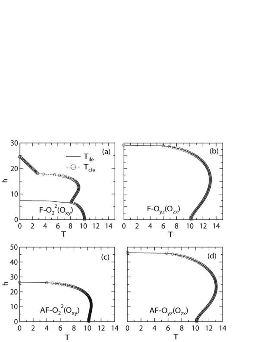
Figure 1: $h$-$T$ phase diagrams for quadrupole ordered states. The solid line determined by linearized mean-field equation. The open circle is given by comparison of free energies between disordered state and corresponding quadrupole ordering state. When these instability points are (not) the same, the transition is of second-order (first-order). It should be noted that $h_{\rm c}^{\prime}(T_{0})=\infty$ in (a-d), which has been shown in Appendix B of Ref. 11.

Table 5: Classification of $\phi^{\Gamma}_{n}$ according to irreducible representations of C_2v, which is point group of tetragonal system in magnetic field parallel to [110]. Here, we note that $\phi^{\Gamma}_{n}$ are bases of multipoles belonging to $\Gamma$ irreducible representation in D_4h point group. The first column shows irreducible representation of C_2v. The second, third, and fourth ones describe quadrupole, $\phi^{\Gamma^{+}}_{n}$, and $\phi^{\Gamma^{-}}_{n}$ belonging to each irreducible representation in C_2v, respectively.

$\Gamma$ (C2v)	quadrupole	$\phi^{\Gamma^{+}}_{n}$ (even)	$\phi^{\Gamma^{-}}_{n}$ (odd)
$\Gamma_{1}$	$O_{2}^{0}$	$\phi^{\Gamma_{1}^{+}}$	$\phi^{\Gamma_{5}^{-}}_{1x}+\phi^{\Gamma_{5}^{-}}_{1y}$
	$O_{\rm xy}$	$\phi^{\Gamma_{4}^{+}}$	$\phi^{\Gamma_{5}^{-}}_{2x}+\phi^{\Gamma_{5}^{-}}_{2y}$
			$\phi^{\Gamma_{5}^{-}}_{3x}-\phi^{\Gamma_{5}^{-}}_{3y}$
$\Gamma_{2}$	$O_{\rm yz}$-$O_{\rm zx}$	$\phi^{\Gamma_{5}^{+}}_{x}-\phi^{\Gamma_{5}^{+}}_{y}$	$\phi^{\Gamma_{4}^{-}}$
$\Gamma_{3}$	$O_{\rm yz}$+$O_{\rm zx}$	$\phi^{\Gamma_{5}^{+}}_{x}+\phi^{\Gamma_{5}^{+}}_{y}$	$\phi^{\Gamma_{2}^{-}}_{1}$
			$\phi^{\Gamma_{2}^{-}}_{2}$
			$\phi^{\Gamma_{3}^{-}}$
$\Gamma_{4}$	$O_{2}^{2}$	$\phi^{\Gamma_{3}^{+}}$	$\phi^{\Gamma_{5}^{-}}_{1x}-\phi^{\Gamma_{5}^{-}}_{1y}$
			$\phi^{\Gamma_{5}^{-}}_{2x}-\phi^{\Gamma_{5}^{-}}_{2y}$
			$\phi^{\Gamma_{5}^{-}}_{3x}+\phi^{\Gamma_{5}^{-}}_{3y}$

IV Discussion of The Second Transition at $T_{1}$

In the previous section, we have analyzed non-magnetic transition at $T_{0}$, and proposed either ferro-$O_{2}^{2}$ or ferro-$O_{xy}$ ordering in system with $\Gamma_{6}$-$\Gamma_{7}$ level scheme. In this section, we provide some proposals for the second transition at $T_{1}$, which is below $T_{0}$. At first, we summarize experimental results below $T_{1}$. Specific heat data showJeevan that a 2^nd order phase transition appears at $T_{1}$. The transition temperature decreases with increasing magnetic field both parallel and perpendicular to [001]. Below $T_{1}$, uniform susceptibility data exhibit a clear difference between the temperature dependence of $\chi_{\rm c}$ and $\chi_{\rm ab}$, which are the uniform susceptibilities in magnetic field parallel and perpendicular to [001], respectively. Here, $\chi_{\rm c}$ seems to be independent of temperature except for a slight decrease just below $T_{1}$, while $\chi_{\rm ab}$ shows a clear cusp at $T_{1}$ in weak magnetic field. From the difference of temperature dependence of $\chi_{\rm c}$ and $\chi_{\rm ab}$ it has been proposed that below T₁ an antiferromagnetic state appears with staggered magnetic moment perpendicular to [001]. In addition magnetization for field perpendicular to [001] has shown a metamagnetic transition. This has been regarded as a spin-flop transition in the $ab$-plane.

From a theoretical point of view, time reversal symmetry must be broken eventually below non-magnetic transition temperature $T_{0}$, in order to release remaining entropy $R\ln{2}$ of the Kramers doublet ground state. In this sense, the antiferromagnetic ordering is reasonable. However, in addition to dipole (magnetic) moments the present model has octupole moments which also break time reversal symmetry. Below the quadrupolar transition temperature $T_{0}$, the point group reduces from D_4h to D_2h in zero magnetic field, because both ferro-$O_{2}^{2}$ and ferro-$O_{xy}$ ordering break only four-fold rotational symmetry. For dipole and octupole moments, there are four one-dimensional irreducible representations in D_2h point group. Among these four irreducible representations, three have respective component of dipole moment $J^{\alpha}$ in addition to two components of octupoles. On the other hand, the remaining irreducible representation has only one octupole component. Let us consider the uniform magnetic susceptibility in pure octupole ordered state. In very weak magnetic field, it is expected that the uniform susceptibility does not considerably decrease below the transition temperature of the octupole ordering, because there is no dipole order parameter in the state. Since this behavior is inconsistent with experimental data of $\chi_{\rm ab}$, we exclude the pure octupole from candidates for the ordered state below $T_{1}$. Therefore, even though we include octupole degrees of freedom, the state below $T_{1}$ seems to be inconsistent with pure octupole ordering, but rather must be an antiferromagnetic state with a considerable magnitude of the dipole moment.

As candidate below $T_{1}$, an antiferromagnetic state will be reasonable from the above discussion of the susceptibility. However, the direction of the staggered moments in the ab plane is still unclear. The direction depends on whether the ordering quadrupole moment below $T_{0}$ is $O_{2}^{2}$ or $O_{xy}$ because their remaining symmetry axis is different. Let us consider ferro-$O_{2}^{2}$ order in magnetic field parallel to [100]. According to Table 3 the allowed directions of magnetic moments in the system are $J^{x}{\bf e}_{x}$, $J^{y}{\bf e}_{y}$, and $J^{z}{\bf e}_{z}$, where ${\bf e}_{x}$, ${\bf e}_{y}$, and ${\bf e}_{z}$ are unit vectors parallel to [100], [010], and [001] directions, respectively. Furthermore the direction of staggered moments in the antiferromagnetic state is perpendicular to [001] axis according to the experimental uniform susceptibility. Therefore, for magnetic transition within the $O_{2}^{2}$ phase, the dipole order parameter should be described by $J^{x}{\bf e}_{x}$ or $J^{y}{\bf e}_{y}$. Likewise within the $O_{xy}$ phase in magnetic field parallel to [110], it should be $J^{x}{\bf e}_{x}\pm J^{y}{\bf e}_{y}$. This means that determination of staggered moment direction can distinguish between quadrupole order of ferro-$O_{2}^{2}$ or ferro-$O_{xy}$ type.

Now we consider the metamagnetic transition, which has been observed in magnetic field perpendicular to [001], starting from an antiferromagnetic state with planar staggered moment. In the present scenario, the antiferromagnetism is regarded to appear below ferro-$O_{2}^{2}$ or ferro-$O_{xy}$ ordering temperature. In these cases the point group reduces from D_4h to D_2h in zero magnetic field. Consequently two-dimensional irreducible representation in D_4h, which involves two planar components of magnetic moment, reduce to the direct sum of two one-dimensional irreducible representations, where each has one planar component of magnetic moment.

Then it is expected that exchange coupling constants between planar components of magnetic moments depend on the in-plane direction. These effective coupling constants are due to RKKY mechanism, therefore their anisotropy will be induced by reconstruction of conduction electron states in the ferro-quadrupolar ordered phase. This exchange anisotropy induced by quadrupole order is the origin of the spin flop transition for $H\perp$[001].

V Mean-field analysis of both ordered phases

From previous discussions, we have two candidates for successive transitions; one scenario is given by ferro-$O_{2}^{2}$ ordering for the first transition at $T_{0}$ before the second transition at $T_{1}$ to antiferromagnetism with staggered moment $J^{x}{\bf e}_{x}$ or $J^{y}{\bf e}_{y}$, and another is ferro-$O_{xy}$ ordering for transition at $T_{0}$ before transition at $T_{1}$ to antiferromagnetism with staggered moment $J^{x}{\bf e}_{x}\pm J^{y}{\bf e}_{y}$. In the following, we assume ferro-$O_{2}^{2}$ ordering for the transition at $T_{0}$, because we cannot distinguish these two possibilities from available experimental data.

V.1 Re-estimation of coupling constants

In the previous section, we have estimated parameter values of model Hamiltonian, such that magnetic anisotropy of uniform susceptibility and non-magnetic transition temperature are reasonably reproduced. However, in that stage, we have assumed that all signs of coupling constants are the same. In the present case, we are considering that the system shows ferro-quadrupole ordering before antiferromagnetic transition. Therefore, we should estimate coupling constants with assumption of ferro-quadrupole transition at $T_{0}$ and antiferromagnetic transition at $T_{1}$. Among these coupling constants, $J^{\Gamma_{1}^{+}}$ and $J^{\Gamma_{3}^{+}}$ are not changed from values used for Fig. 1(a). On the other hand, we choose value of $J^{\Gamma_{5}^{-}}$ as antiferromagnetic transition appears at $T_{1}$=6.5K in zero magnetic field. In addition, magnitudes of other coupling constants are chosen to be small with $\alpha^{\Gamma^{\prime}}$=0.25 ($\Gamma^{\prime}$=$\Gamma_{4}^{+}$, $\Gamma_{5}^{+}$, $\Gamma_{2}^{-}$, $\Gamma_{3}^{-}$, and $\Gamma_{4}^{-}$), so that unobserved phases are suppressed which would appear if $\alpha^{\Gamma^{\prime}}$ were larger. Furthermore, considering that coupling constant between x-components of magnetic moment is different from correspondence between y-components of magnetic moment in ferro-$O_{2}^{2}$ ordering state, we will reduce magnitude of coupling constant between $\phi^{\Gamma_{5}^{-}}_{3y}$. In Table 4, we summarize the revised values of coupling constants.

V.2 Phase diagram

At first, we construct $H$-$T$ phase diagram in magnetic field parallel to [001]. As we have mentioned in §III.A, in order to find the transition line, we use two kinds of procedures; one is given by linearized mean-field equation, while the other is determined by comparison of free energies of different states. In Fig. 3, we show calculated $H$-$T$ phase diagram in magnetic field parallel to [001]. In the high field region of the phase diagram, level crossing between $\Gamma_{6}$ and $\Gamma_{7}$ states is obtained in terms of larger magnitude and negative sign of $g$-factor of the $\Gamma_{7}$ state. The transition at $T_{0}$ is of second-order, and $T_{0}$ decreases with increasing magnetic field. The transition at $T_{1}$ is second-order transition from ferro-$O_{2}^{2}$ phase to coexistent phase of ferro-$O_{2}^{2}$ and antiferromagnetism. Here, dashed line shows instability of paramagnetic state to ferro-$O_{2}^{2}$ state, while dotted line is instability line of paramagnetic state to antiferromagnetic state with staggered moment parallel to [100]. The dashed line is very different from instability line shown in Fig. 1, since coupling constant between field induced $\phi^{\Gamma_{4}^{-}}$ is changed from ferro-coupling to antiferro-coupling. Comparing these instability lines with the transition line to the coexistent phase, ferro-$O_{2}^{2}$ and antiferromagnetism are cooperative to each other and stabilize the coexistent phase.

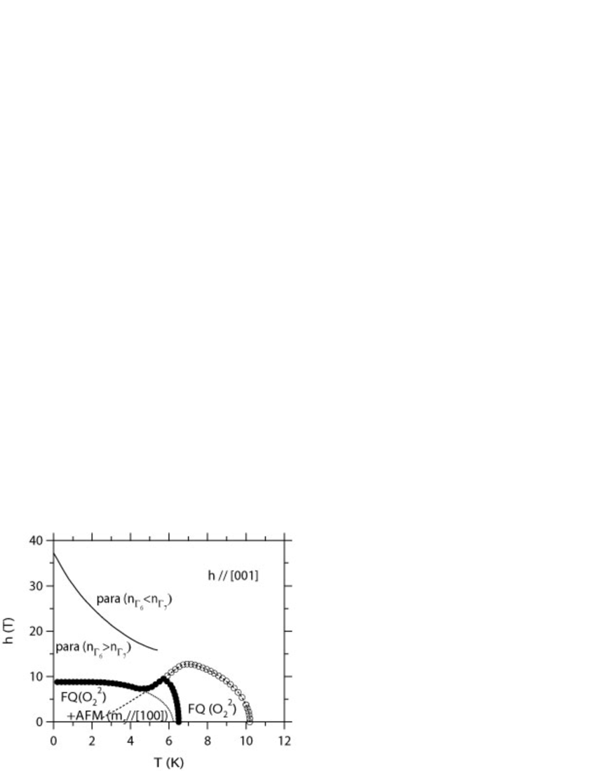
Figure 3: $h$-$T$ phase diagram in magnetic field parallel to [001]. The solid line shows level crossing temperature. The dashed and dotted lines are instability lines of disordered state to ferro-$O_{2}^{2}$ state and antiferromagnetic state with staggered moment parallel to [100], respectively. The open circle corresponds to transition point from disordered state to ferro-$O_{2}^{2}$ ordered state. The solid circle corresponds to transition point from paramagnetic state (including ferro-$O_{2}^{2}$ ordered state) to coexistent state of both ferro-$O_{2}^{2}$ moment and staggered magnetic moment parallel to [100]. These circles are determined by comparison of free energies.

In Fig. 4, we show calculated $H$-$T$ phase diagram in magnetic field parallel to [100]. In this figure, $T_{0}$ is not a transition temperature but the crossover temperature from usual paramagnetic phase in high temperature region to disordered phase with considerable ferro-$O_{2}^{2}$ moment in low temperature region, where the crossover temperature is determined by inflection point of temperature dependence of $C/T$. The crossover temperature increases with increasing magnetic field. In order to consider low temperature state, we take into account reduced coupling constant between $J^{y}$, which is mentioned in §.IV. By the anisotropic magnetic interaction, we have two antiferromagnetic phases. Here, low field phase has staggered moment parallel to the magnetic field, while high field phase has perpendicular component to the magnetic field. Therefore, spin-flop transition is obtained, where the transition between these phases is of first-order. If we use the same coupling constant as the one between $J^{x}$, low field antiferromagnetic phase disappears. In the inset of Fig. 4, metamagnetic transition corresponding to the spin-flop is obtained.

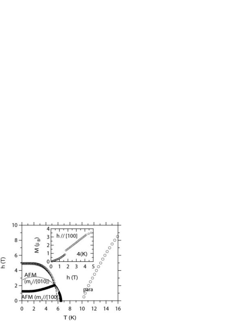
Figure 4: $h$-$T$ phase diagram in magnetic field parallel to [100]. The open circle shows crossover temperature determined by inflection point of temperature dependence of $C/T$. The dotted and dashed lines are instability lines of disordered state to antiferromagnetic state with staggered moment parallel to [100] and parallel to [010], respectively. The up-triangle and down-triangle correspond to transition point from disordered state to antiferromagnetic state with staggered moment parallel to [100] and parallel to [010], respectively, which are determined by comparison of free energies. Inset shows magnetization in field parallel to [100].

V.3 Specific heat

In specific heat data, there are some anomalous features in the temperature and field dependences. In magnetic field parallel to [001], specific heat jumps are observed at $T_{0}$ and $T_{1}$, and these transition temperatures decrease with increasing magnetic field. In magnetic field perpendicular to [001], the anomaly at the non-magnetic transition reduces to a hump and broadens with increasing magnetic field. In order to compare with the experimental data, we calculate specific heat in magnetic field, based on the mean-field solution.

In order to calculate specific heat, we first provide expression of internal energy $E_{\rm I}$, as follows:

$$E_{\rm I}=\sum_{\bf j}\sum_{n}\epsilon_{n}\langle\psi^{\Gamma_{1}}_{{\bf j}n}\rangle-\sum_{{\bf i}\neq{\bf j}}\sum_{\Gamma,n}J^{\Gamma}_{{\bf i}-{\bf j}n}\langle\psi^{\Gamma}_{{\bf i}n}\rangle\langle\psi^{\Gamma}_{{\bf j}n}\rangle,$$ (26)

where the first term of right hand side exhibits contributions from CEF term and Zeeman term. Then, specific heat is given by temperature derivative of the internal energy as

$$C=\sum_{\bf j}\sum_{n}\epsilon_{n}\frac{d\langle\psi^{\Gamma_{1}}_{{\bf j}n}\rangle}{dT}$$

$$\hskip 14.22636pt-\sum_{{\bf i}\neq{\bf j}}\sum_{\Gamma,n}2J^{\Gamma}_{{\bf i}-{\bf j}n}\langle\psi^{\Gamma}_{{\bf i}n}\rangle\frac{d\langle\psi^{\Gamma}_{{\bf j}n}\rangle}{dT},$$ (27)

with equation of temperature derivative of $\langle\psi^{\Gamma}_{{\bf j}n}\rangle$

$$\frac{d\langle\psi^{\Gamma}_{{\bf j}n}\rangle}{dT}=\sum_{n^{\prime}}\frac{\epsilon_{n^{\prime}}}{T}\chi^{\Gamma_{1}\Gamma}_{{\bf j}n^{\prime}n}$$

$$\hskip 14.22636pt-\sum_{{\bf i}(\neq{\bf j})}\sum_{\Gamma^{\prime},n^{\prime}}2J^{\Gamma^{\prime}}_{{\bf i}-{\bf j}n^{\prime}}(\frac{\langle\psi^{\Gamma^{\prime}}_{{\bf i}n^{\prime}}\rangle}{T}-\frac{d\langle\psi^{\Gamma^{\prime}}_{{\bf i}n^{\prime}}\rangle}{dT})\chi^{\Gamma^{\prime}\Gamma}_{{\bf j}n^{\prime}n}.$$ (28)

where $\chi^{\Gamma^{\prime}\Gamma}_{{\bf i}n^{\prime}n}$ is given by the sublattice dependent expression

$$\chi^{\Gamma^{\prime}\Gamma}_{{\bf i}n^{\prime}n}=\int^{1/T}_{0}d\tau\hskip 2.84526pt\langle\psi^{\Gamma^{\prime}}_{{\bf i}n^{\prime}}(\tau)\psi^{\Gamma}_{{\bf i}n}\rangle-\frac{\langle\psi^{\Gamma^{\prime}}_{{\bf i}n^{\prime}}\rangle\langle\psi^{\Gamma}_{{\bf i}n}\rangle}{T}.$$ (29)

Using these expressions, we calculate the specific heat of the system in a magnetic field. In Fig. 5(a) and 5(b), we show temperature dependences of specific heat for field parallel to [001] and [100] directions, respectively. In Fig. 5(a), there are two specific heat jumps corresponding to transitions to ferro-$O_{2}^{2}$ state at $T_{0}$ and to coexistent state at $T_{1}$. In addition, field dependence of the specific heat is very weak in low field region. In Fig. 5(b), only specific heat jump is due to transition to antiferromagnetic state at $T_{1}$, while hump structure related to the crossover temperature at $T_{0}$ broadens with increasing magnetic field. This means that the ferro-$O_{2}^{2}$ moment is induced by magnetic field parallel to [100] as shown in Table 3 and no symmetry breaking at $T_{0}$ takes place for $H>0$.

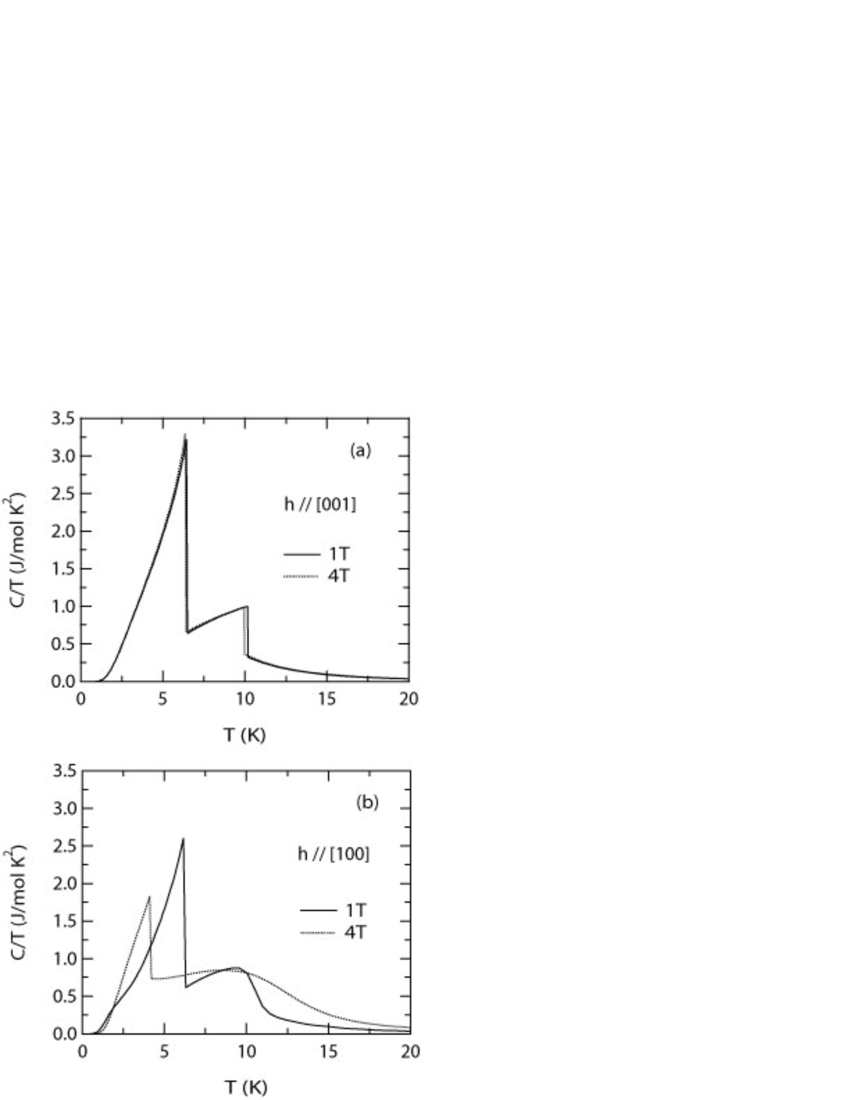
Figure 5: Temperature dependences of specific heat in magnetic field parallel to [001] (a) and parallel to [100] (b). The solid and dotted lines correspond to 1T and 4T, respectively.

V.4 Uniform susceptibility

The experimental data of uniform susceptibility exhibits characteristic properties. In the magnetic field perpendicular to [001], uniform susceptibility does not show anomaly at $T_{0}$, except for the slight increase of magnitude of the temperature derivative at $T_{0}$ in low field region. On the other hand, temperature dependence of uniform susceptibility in magnetic field parallel to [001] has a plateau-like behavior between $T_{0}$ and $T_{1}$. In addition, the temperature dependence is almost insensitive to the magnetic field up to 3T. In order to analyze uniform susceptibility, we give expressions of the quantity in magnetic field parallel to [001] and [100]. For direct comparison with experimental data in finite magnetic field, magnetization divided by magnitude of the field is used as uniform susceptibility, instead of the Kubo formula of susceptibility from linear response theory. Then, uniform susceptibility $\chi_{\rm c}$ in magnetic field parallel to [001] is given by

$$\chi_{\rm c}=\frac{g_{J}\mu_{\rm B}}{h}\langle J^{\rm z}\rangle,$$ (30)

while uniform susceptibility in magnetic field parallel to [100] is similarly obtained from

$$\chi_{\rm a}=\frac{g_{J}\mu_{\rm B}}{h}\langle J^{\rm x}\rangle,$$ (31)

where $J^{\rm z}$ and $J^{\rm x}$ are given by eqs. (6) and (7), respectively.

In Fig. 6(a), we show calculated temperature dependence of uniform susceptibility in magnetic field parallel to [001]. Anomalies due to two transitions at $T_{0}$ and $T_{1}$ are obtained. Here, we note that plateau in temperature dependence between $T_{0}$ and $T_{1}$ is due to moderate coupling constant between octupoles $\phi^{\Gamma_{4}^{-}}$, which are induced by the magnetic field, while temperature independent behavior well below $T_{1}$ reflects existence of staggered moment perpendicular to the magnetic field. In addition, the uniform susceptibility hardly has field dependence at least in the low field region. In Fig. 6(b), we show temperature dependence of uniform susceptibility in magnetic field parallel to [100]. From the figure it shows slight upturn around crossover temperature $T_{0}$. In magnetic field of 1T, it shows a cusp at transition temperature to antiferromagnetism with staggered moment parallel to the magnetic field. With increase of magnetic field to 4T, the uniform susceptibility shows temperature independent behavior below transition temperature to antiferromagnetism with staggered moment perpendicular to the magnetic field. The different of behavior below antiferromagnetic transition temperature is due to the spin-flop transition, as shown in Fig. 4.

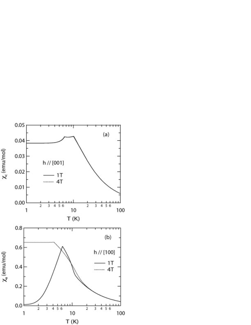
Figure 6: Temperature dependences of uniform susceptibilities in magnetic field parallel to [001] (a) and parallel to [100]. The solid and dotted lines correspond to 1T and 4T, respectively.

VI discussion and summary

Before we summarize, we would like to comment on a few points. In the previous section, we have calculated specific heat, uniform susceptibility, and phase diagram with assumption of ferro-$O_{2}^{2}$ ordering at $T_{0}$. Comparing our results with experimental data of YbRu₂Ge₂, the present model not only explains the experimental data qualitatively, but also gives quantitative agreement in specific heat jumps. Therefore, ferro-$O_{2}^{2}$ ordering at $T_{0}$ above antiferromagnetic transition temperature $T_{1}$ will be one of promising candidate for non-magnetic transition of YbRu₂Ge₂. However, we have proposed either ferro-$O_{2}^{2}$ or ferro-$O_{xy}$ ordering for the transition at $T_{0}$ in §. III. Considering that both candidates are ferro-ordering states of quadrupoles, in order to identify the non-magnetic state among the two candidates, it will be useful to carry out ultrasonic and x-ray scattering experiments , because ferro-quadrupole couples with lattice distortion. From this point of view, it is desirable to confirm the crystal structure below $T_{0}$.

Related to property of non-magnetic ordering state, it has been recently reported that Ru-NQR spectrum may not be affected by the non-magnetic transitionMukuda . With respect to this result, taking into account positions of Yb and Ru ions, if dominant quadrupole of Ru-nucleus is either $O_{2}^{0}$ or $O_{2}^{2}$, ferro-$O_{xy}$ ordering of Yb³⁺ does not change Ru-NQR spectrum by the transition. On the other hand, if quadrupole of Ru-nucleus is $O_{xy}$, ferro-$O_{2}^{2}$ ordering does not change the spectrum by the transition. Furthermore, if quadrupole of Ru-nucleus is either $O_{yz}$ or $O_{zx}$, both ferro-$O_{2}^{2}$ ordering and ferro-$O_{xy}$ ordering do not change the spectrum. In order to identify the type of quadrupole ordering, it is required to clarify the quadrupole of Ru-nucleus.

Furthermore, in recent uniform susceptibility data, it is shown that behavior of uniform susceptibility in magnetic field parallel to [100] is similar as that in magnetic field parallel to [110], and these uniform susceptibilities have finite value at very low temperature. Based on the present model with assumption of either ferro-$O_{2}^{2}$ or ferro-$O_{xy}$ ordering at $T_{0}$, one of these uniform susceptibility will vanish at 0K in small magnetic field region by development of staggered magnetic moment parallel to the magnetic field. Considering that finite values are observed for both uniform susceptibilities in very low temperature region, the ordering wave vector of magnetic moments will be an incommensurate one. Therefore, it is desirable to carry out neutron scattering experiment to clarify the magnetic state of the compound.

Finally, we comment on effect of multipolar fluctuations. The effect has been investigated in CeB₆ by ShiinaShiina2 . In the paper, it has been shown that the multipolar fluctuation are enhanced by approaching the system to the SU(4) symmetric limit. In YbRu₂Ge₂, it is considered that the tetragonal anisotropy like splitting energy $\Delta$ between $\Gamma_{6}$ and $\Gamma_{7}$ states breaks the SU(4) symmetry inherently. Therefore we do not expect that the multipolar fluctuations change qualitatively behaviors suggested by the mean-field theory.

In summary, in order to explain properties of YbRu₂Ge₂, we have introduced a quasi-degenerate localized model consisting of CEF term, Zeeman term, and exchange term of multipoles. Classifying multipoles according to irreducible representations of corresponding point group, we have developed a mean-field theory for the model. Considering that the specific heat jump broadens with increasing magnetic field perpendicular to [001], we have proposed that for the non-magnetic transition, only ferro-$O_{2}^{2}$ and ferro-$O_{xy}$ orderings are possible candidates. Furthermore, it has been shown that these ferro-quadrupole orderings are only available and essentially of the induced type, when the lower two CEF states consist of one $\Gamma_{6}$ and one $\Gamma_{7}$ doublets in zero magnetic field. With assumption of ferro-$O_{2}^{2}$ ordering at $T_{0}$, we have calculated specific heat, uniform susceptibility, and phase diagram, where anisotropic exchange interaction between planar components of magnetic moments is introduced as an effect of the ferro-quadrupole ordering. The calculated results have been shown to explain experimental data consistently. In order to clarify the property of YbRu₂Ge₂ completely and refine the set of coupling constants, it is desirable to carry out more detailed experiments like elastic constant measurements and neutron diffraction in applied magnetic field.

References

- (1) T. Fujita, M. Suzuki, T. Komatsubara, S. Kunii, T. Kasuya, and T. Ohtsuka, J. Phys. Soc. Jpn. 35, 569 (1980).
- (2) M. Takigawa, H. Yasuoka, T. Tanaka, and Y. Ishizawa, J. Phys. Soc. Jpn. 52, 728 (1983).
- (3) J. M. Effantin, J. Rossat-Mignod, P. Burlet, H. Bartholin, S. Kunii, and T. Kasuya, J. Magn. Magn. Mater. 47&48, 145 (1985).
- (4) D. Mannix, G. H. Lander, J. Rebizant, R. Caciuffo, N. Bernhoeft, E. Lidstrm, and C. Vettier, Phys. Rev. B60, 15187 (1999).
- (5) J. A. Paixo, C. Detlefs, M. J. Longfield, R. Caciuffo, P. Santini, N. Bernhoeft, J. Rebizant, and G. H. Lander, Phys. Rev. Lett. 89, 187202 (2002).
- (6) S. W. Lovesey, E. Balcar, C. Detlefs, G. van der Laan, D. S. Sivia, and U. Staub, J. Phys.: Condens. Matter 15, 4511 (2003).
- (7) Y. Tokunaga, Y. Homma, S. Kambe, D. Aoki, H. Sakai, E. Yamamoto, A. Nakamura, Y. Shiokawa, R. E. Walstedt, and H. Yasuoka, Phys. Rev. Lett. 94, 137209 (2005).
- (8) J. W. Ross and D. J. Lam, J. Appl. Phys. 38, 1451 (1967).
- (9) P. Erds, G. Solt, Z. Zolnierek, A. Blaise, and J. M. Fournier, Physica B&C 102B, 164 (1980).
- (10) H. S. Jeevan, C. Geibel, and Z. Hossain, Phys. Rev. B73, 020407(R) (2006).
- (11) R. Shiina, H. Shiba, and P. Thalmeier, J. Phys. Soc. Jpn. 66, 1741 (1997).
- (12) R. Shiina, H. Shiba, and O. Sakai, J. Phys. Soc. Jpn. 68, 2105 (1999).
- (13) K. Kubo and T. Hotta, Phys. Rev. B71, 140404(R) (2005).
- (14) G. T. Trammell, J. Appl. Phys. 31, 362S (1960). Phys. Rev. 131, 932 (1963).
- (15) B. Bleaney, Proc. Roy. Soc. (London) 276A, 19 (1963).
- (16) C. Geibel, private communication.
- (17) In Fig. 1(a), we can see the sign of the level cross around 20T. Here, we should note that this first-order transition is different from non-magnetic transition observed in YbRu2Ge2, because this transition is not expected in low-field region.
- (18) H. Mukuda, private communication.
- (19) R. Shiina, J. Phys. Soc. Jpn. 70, 2746 (2001).