Numerical simulations of HH 555

Abstract

We present 3D gasdynamic simulations of the Herbig Haro object HH 555. HH 555 is a bipolar jet emerging from the tip of an elephant trunk entering the Pelican Nebula from the adjacent molecular cloud. Both beams of HH 555 are curved away from the center of the H II region. This indicates that they are being deflected by a side-wind probably coming from a star located inside the nebula or by the expansion of the nebula itself. HH 555 is most likely an irradiated jet emerging from a highly embedded protostar, which has not yet been detected.

In our simulations we vary the incident photon flux, which in one of our models is equal to the flux coming from a star 1 pc away emitting 5$\times$10⁴⁸ ionizing (i. e., with energies above the H Lyman limit) photons per second. An external, plane-parallel flow (a “side-wind”) is coming from the same direction as the photoionizing flux. We have made four simulations, decreasing the photon flux by a factor of 10 in each simulation. We discuss the properties of the flow and we compute H$\alpha$ emission maps (integrated along lines of sight). We show that the level of the incident photon flux has an important influence on the shape and visibility of the jet. If the flux is very high, it causes a strong evaporation of the neutral clump, producing a photoevaporated wind traveling in the direction opposite to the incident flow. The interaction of the two flows creates a double shock “working surface” around the clump protecting it and the jet from the external flow. The jet only starts to curve when it penetrates through the working surface.

1 Introduction

Many new Herbig Haro objects have been discovered in recent years by various deep imaging surveys (i. e. Bally & Reipurth 2001, 2003, Reipurth et al. 2004 and Walawander, Bally & Reipurth 2005). These objects come in different forms and shapes. Some of them are seen as barely observable spots, others appear in the form of chains of knots or as symmetric or asymmetric jets. The jets can be straight or curved (see for example the jets described in Bally & Reipurth 2001). The curving of the jets is usually interpreted as the interaction of the jet with an enviorment in relative motion with respect to the outflow source. Numerical simulations have been made for the curved jets in the Orion Nebula (M42) by Masciadri & Raga (2001). The problem of a jet in a sidewind has also been aproached analytically and experimentally. Cantó & Raga (1995) found an analytical solution for the shape of the jet, while Lebedev et al. (2004) studied jet deflection by crosswinds in laboratory.

In the present paper, we simulate a peculiar Herbig Haro object known as HH 555 located in the Pelican Nebula (IC4050), discovered by Bally & Reipurth (2003) (see Figure 1). HH 555 is a bipolar jet emerging from the tip of an elephant trunk embedded in the nebula. The jet and counterjet both curve away from the ionizing source, indicating that they might be interacting with a stellar wind or with the expanding H II region.

We carry out 3D gasdynamical simulations in which we include the ionizing photon flux (from $\theta$ Orionis) and the expanding H II region (modeled as a plane-parallel flow entering the computational grid in a direction parallel to the impinging ionizing photon flux) interacting with the elephant trunk (modeled as a dense cylinder+spherical cap, neutral structure). From close to the tip of the elephant trunk, a bipolar outflow is injected, with an axis at an angle to the impinging, ionizing flux. We present the results for four models exploring different values for the impinging ionizing photon flux (but with otherwise identical parameters), and compare the results in a qualitative way with the observations of HH 555.

The paper is organized as follows. In section 2, we describe the properties of HH 555, as derived by Bally & Reipurth (2003). In section 3, we present the numerical simulations, and predictions of H$\alpha$ emission maps are discussed in section 4. Finally, the conclusions are given in section 5.

2 Physical properties of HH 555

Bally & Reipurth (2003) give the following description of the elephant trunk and HH 555: the elephant trunk is a $4^{\prime}$ long filament of neutral gas, which penetrates into the Pelican Nebula. It shows a dense condensation at its tip, with a $\sim 20^{\prime\prime}$ diameter. Two curved flows emerge from it in a direction almost perperdicular to the elephant trunk. They are the southern and the northern outflow lobes, which have lengths of $\sim 25^{\prime\prime}$. The flows bend at an angle of 25^∘ in the direction away from the center of the Pelican Nebula, giving it a “C”-shaped symmetry. The angular width of the jets is of $\approx 2^{\prime\prime}$, which for an assumed distance of 600 pc implies jet diameters of 1200 AU.

The radial velocity measurements of the southern jet (the spectra for the northern jet have not been obtained yet) give values of up to $-80$ km s^-1 with respect to the background emission of the Pelican Nebula. From the [S II] doublet ratio, $I(\lambda 6717)/I(\lambda 6731)$, the electron density was estimated to be $n_{e}\approx$600 cm^-3 in contrast to $n_{e}\approx$200 cm^-3 for the background nebula. From these data the mass-loss rate is estimated to be $\dot{M}=1.4\times 10^{-7}$ M_⊙ yr^-1. The source of the jets is probably highly embedded inside the elephant trunk, since it could not be detected at infrared wavelengths.

3 The Numerical Simulations

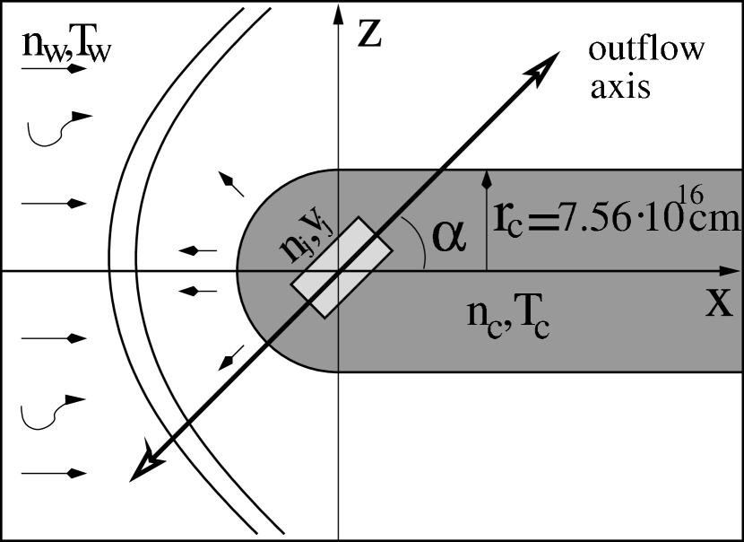
Figure 2: A schematic presentation of the numerical setup. The ionizing photon flux and an ionized, plane-parallel flow are impinging from the left, along the $x$-axis. The neutral, elephant trunk structure has the form of a cylinder+spherical cap. From the center of the cap, a bipolar jet emerges forming an angle $\alpha$ with the $x$-axis. For a high enough impinging photon flux, the interaction of the photoevaporated flow with the impinging plane-parallel wind creates a two-shock structure around the neutral clump.

In order to simulate the HH 555 outflow, we have carried out 3D numerical simulations in which we include a number of elements, which are shown in the schematic diagram of Figure 2. These elements are:

• a plane-parallel ionizing photon flux $F_{*}$ which enters the computational grid in the $+x$-direction. We compute 4 models (models 1 through 4) with $F_{*}=(4.2,42,420,4200)\times 10^{7}$ cm^-2s^-1 (respectively). The highest of these fluxes corresponds to an unshielded ionizing source with an ionizing photon rate of $S_{*}=5\times 10^{48}$ s^-1 located at a distance of 1 pc from the center of the computational grid. The lower values of $F_{*}$ could be the result of larger distances to the ionizing photon source, or could be interpreted as the effect of absorption (due to dust or to hydrogen photoionization) in the material between the source and the simulated region. In all models, a black body spectral distribution with a $T_{*}=40000$ K temperature is assumed,

• an expanding photoionized region, modeled as a plane-parallel inflow (also in the $+x$-direction) of gas with a $v_{w}=50$ km s^-1 velocity, $n_{w}=10$ cm^-3 density and $T_{w}=10^{4}$ K temperature. The expanding H II region is identical in the four computed models,

• an “elephant trunk”, modeled as a neutral, initially stationary cylinder+spherical cap structure aligned with the $x$-axis, with a $r_{c}=7.56\times 10^{16}$ cm radius. This neutral structure has a $n_{c}=10^{4}$ cm^-3 density and $T_{c}=100$ K temperature,

• a bipolar outflow with an initial radius $r_{j}=3\times 10^{15}$ cm, velocity $v_{j}=100$ km s^-1, density $n_{j}=600$ cm^-3 and temperature $T_{j}=1000$ K. The outflow is imposed in a cylinder of radius $r_{j}$ and length $2r_{j}$ (with velocities of $\pm v_{j}$ along the symmetry axis of this cylinder, in the top and bottom halfs of the cylinder, respectively). The bipolar outflow is initially neutral. The center of the cylinder coincides with the center of the spherical cap (which forms the end of the neutral elephant trunk, see above), and also with the center of the $(x,y,z)$ coordinate system. The outflow axis lies on the $xz$-plane and forms an angle $\alpha=70^{\circ}$ with the $x$-axis (see Figure 2).

The numerical simulations are computed with the “yguazú-a” adaptive grid code (see the description of Raga, Navarro-González & Villagrán-Muniz 2000), using the version of the code described by Raga & Reipurth (2004). This version of the code solves the 3D gasdynamic equations together with a single rate equation for neutral hydrogen. Radiative recombination, and collisional and photo-ionizations are included. A simultaneous solution is made of the transfer of ionizing photons (at the Lyman limit) along the $x$-axis. A parametrized cooling function (calculated as a function of the ionization fraction, density and temperature) and the heating due to photoionization of H are also included in the energy equation (see Raga & Reipurth 2004). We should note that because of our “Lyman limit only” approximation to the radiative transfer, the spectral distribution (which we assume to be a black body with $T_{*}=40000$ K, see above) only appears in the photoionization heating term (see Cantó et al. 1998).

From the results of our simulations, we compute H$\alpha$ emission maps by integrating the H$\alpha$ emission coefficient along lines of sight. We compute this emission coefficient by adding the contributions of the “case B” recombination cascade and the collisional excitations from the $n=1$ level of H.

For our computations, we have chosen a 5-level, binary adaptive grid with a maximum resolution of $1.27\times 10^{15}$ cm (along the three axes). The computational domain has an extent of $(6.5,3.25,6.5)\times 10^{17}$ cm along the $(x,y,z)$-axes (respectively). Transmission conditions are imposed on all boundaries except for the $-x$ boundary, in which the “expanding H II region” inflow condition (see above) is imposed.

In our simulations, the expanding H II region (with a $n_{w}=10$ cm^-3 density and a $v_{w}=50$ km s^-1 velocity) forms a bow shock against the photoevaporated wind from the elephant trunk. From the models of Hartigan et al. (1987), we find that a plane-parallel, stationary shock model with a preshock density of 10 cm^-3 and a 50 km s^-1 shock velocity has a cooling distance (to $10^{4}$ K) $d_{c}\approx 6\times 10^{14}$ cm. At the head of the leading bow shock of the jet, we have a shock velocity $\sim v_{j}=100$ km s^-1, and a preshock density $>10$ cm^-3 (corresponding to the shocked expanding H II region). For a shock velocity of 100 km s^-1 and a 10 cm^-3 preshock density, the models of Hartigan et al. (1987) give a cooling distance (to $10^{4}$ K) of $1.2\times 10^{15}$ cm. These estimates show that the post-shock cooling distances are not resolved in our simulations. However, the contribution of these regions to the H$\alpha$ emission of the photoionized flow should be relatively small (see, e. g., Masciadri & Raga 2004).

The simulations start with the expanding H II region occupying all of the domain, except for the region with the elephant trunk. The embedded outflow is also “turned on” at this initial time. The simulations proceed to a total integration time 3000 years.

4 Results

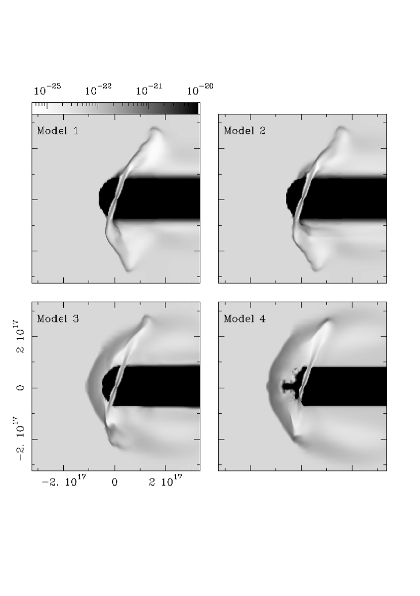
Figure 3: Density on the midplane of the simulation obtained from simulations with different impinging hydrogen-ionizing photon fluxes. For each model we show a time slice corresponding to a 3000 yr simulation time. The extent of the computational domain is $(6.5,3.25,6.5)\times 10^{17}$ cm along the $(x,y,z)$-axes (respectively) and the maximum resolution of the adaptive grid is of $1.27\times 10^{15}$ cm. The photon flux and the expanding H II region impinge from the left, parallel to the symmetry axis of the neutral elephant trunk. The jet is ejected at an angle of 70^∘ with respect to the $x$-axis. The photon flux has values $F_{*}=(4.2,42,420,4200)\times 10^{7}$ cm^-2s^-1 for models 1 through 4 (respectively). The density stratifications are depicted with the logarithmic greyscale shown by the top bar, in units of g cm^-3. The axes are labeled in cm.

The results of our simulations are shown in Figures 3 and 4. We have calculated four models with basically identical initial setup, except for the incident photon flux. Our goal was to determine the influence of the flux on the shape and visibility of the jet. The values of the photon flux are $F_{*}=(4.2,42,420,4200)\times 10^{7}$ cm^-2s^-1 for models 1 through 4 (respectively). The photon flux in Model 4 is equal to the flux coming from a star 1 pc away emitting 5$\times$10⁴⁸ ionizing photons per second (which corresponds to an ionizing source such as $\theta$ Orionis). The lower values of $F_{*}$ could be the result of the interstellar absorption in the material between the source and the simulated object or could be a consequence of larger distances to the ionizing photon source.

4.1 The neutral clump

Figure 3 shows the density stratifications on the $xz$-plane (i. e., the plane on which lies the outflow axis, see § 3) after a $t=3000$ yr integration time for models 1 through 4. These stratifications show the shape of the bipolar outflow and of the eroded neutral clump.

In models 1 and 2, the expanding H II region (impinging on the neutral clump along the $x$-axis) forms a bow shock against the neutral clump, and against the side of the outflow which emerges from the clump. The clump material which is photoionized by the impinging ionizing photon flux is confined to a very narrow region (surrounding the neutral clump) by the expanding H II region. The shape of the clump changes because of the interaction with the expanding H II region and the ionizing photon flux. Its dimension along the $x$-axis is reduced as the time-integration progresses.

As the impinging photoionizing flux is increased (models 3 and 4), so does the amount of photoevaporated material. In models 3 and 4 the interaction of the photoevaporated wind with the expanding H II region forms a detached two-shock structure. In model 3, and more dramatically in model 4, the neutral structure is eroded as it ejects a photoevaporated wind. This photoevaporation is stronger in model 4, and for this model we already see the axial collapse (always obtained in simulations of the photoevaporation of neutral clumps, see, e. g., Mellema et al. 1998) at a $t=3000$ yr integration time.

The results from our models can be interpreted in terms of the analytic photoevaporated wind/expanding H II region interaction model of Henney et al. (1996) and Raga et al. (2005). These authors define a “high ionizing photon flux” and a “low ionizing photon flux” regime. In the first regime a detached, two-shock structure is created by the interaction of the photoevaporated wind with the impinging H II region, while in the second regime the photoionized clump material is confined to a thin shell around the neutral clump.

In the “high ionizing photon flux” regime, the distance (along the symmetry axis) between the two-shock structure and the center of the neutral clump is

$$r_{w}=\lambda^{1/2}r_{0},$$ (1)

where $r_{0}$ is a radius of the neutral structure. The dimensionless parameter $\lambda$ is given by

$$\lambda=\frac{F_{0}c_{I}}{n_{w}v^{2}_{w}},$$ (2)

where $F_{0}$ is the photon flux which actually arrives to the surface of the neutral clump at a given time, $c_{I}$ is the sound speed of the photoevaporated wind ($\sim$10 km s^-1), and $n_{w}$ and $v_{w}$ are the density and the velocity of the impinging expanding H II region.

For $\lambda>1$, the two-shock structure is detached and the flow is in the “high ionizing photon flux” regime. For $\lambda<1$, the flow is in the “low ionizing photon flux” regime. In the case of our models, we calculated analytical values of $\lambda$ using the model of Raga et al. (2005), obtaining $\lambda=0.14$, 0.80, 3.35 and 8.32 for models 1 through 4 (respectively). Consistently with these $\lambda$ values, in our numerical simulations we obtain detached shock structures only for models 3 and 4.

In Figure 4 we show H$\alpha$ emission maps (obtained by integrating the H$\alpha$ emission coefficient along the $y$-axis, without considering the extinction within the elephant trunk). In the case of models 1 and 2, very little emission is seen from the region of interaction between the clump and the impinging ionizing photon flux and expanding H II region. For these two models, the emission is dominated by the jet (described in §4). The converse is true for models 3 and 4, in which the H$\alpha$ emission is dominated by the photoevaporated wind and the region of interaction between the photoevaporated wind and the expanding H II region.

4.2 The jet

The shape of the jet can be seen in the density stratifications shown in Figure 3. In the case of models 1 and 2, once outside the neutral clump, the outflow lobes have different shapes. In both lobes, the jet begins to curve as soon as it exits the neutral elephant trunk. The bottom lobe (travelling in the $-z$ direction) has a much stronger curvature, changing its direction of propagation from the $-x$ to the $+x$ direction.

In the case of the models 3 and 4, the jets emerge from the neutral region with basically unchanged directions of propagation. This is due to the fact that the downward directed lobe is travelling within a region occupied by the photoevaporated wind (ejected from the neutral structure), which has a direction of motion which is approxmately parallel to the jet. The upward directed jet is travelling into a low density region, which is shielded from the expanding H II region by the detached, two-shock interaction region.

Further out from the outflow source, the jets interact with the two-shock structure (resulting from the photoevaporated wind/expanding H II region interaction). In this interaction, the downward directed jet curves substantially. The upward directed jet curves in a less substantial way as it penetrates the two-shock interaction region.

The H$\alpha$ emission maps (Figure 4) show that in models 1 and 2 the emission is dominated by the region in which the expanding H II region interacts with the jet beam. The emission has a strong resemblance to the jet/sidewind interaction models of Masciadri & Raga (2001).

In models 3 and 4, the H$\alpha$ emission is dominated by the photoevaporated wind and the wind/expanding H II region interaction, two-shock structure (see §3 and Figure 4). For model 4, only the upwards directed jet is visible where it penetrates the two-shock structure (at $z\sim 2\times 10^{16}$ cm). For model 3, both outflow lobes are visible, superimposed on the wings of the two-wind interaction bow shock.

5 Conclusions

In this paper, we simulate the peculiar Herbig Haro object HH 555, located in the Pelican Nebula (IC4050), which is thought to be irradiated by nearby stars and deflected by an expanding H II region.

We computed four 3D simulations of a bipolar jet emerging from the tip of a neutral “elephant trunk”. The elephant trunk is aligned with an impinging ionizing photon flux and a wind of ionized material (i. e., the expanding H II region). The bipolar outflow emerges at an $\alpha=70^{\circ}$ angle with respect to the axis of the elephant trunk. All of these elements are taken directly from the observations of HH 555 of Bally & Reipurth (2003).

In our models, we explore the effect of varying the impinging ionizing photon flux $F_{*}$ (while keeping constant all of the other model parameters). We have computed 2 models (models 1 and 2) in the “low ionizing flux” regime (see Henney et al. 1996), in which the expanding H II region forms a bow shock against the surface of the neutral structure, and two models in the “high ionizing photon flux” regime (models 3 and 4), in which a detached, two-shock structure is formed as a result of the interaction between a photoionized wind and the expanding H II region.

In models 1 and 2, the expanding H II region directly interacts with the bipolar outflow, starting at the point in which the jets emerge from the neutral elephant trunk. The curvature of the jets in these two models is similar to the one observed in HH 555, and the predicted H$\alpha$ emission maps (see Figure 4) have a strong qualitative resemblance to the observed object.

In models 3 and 4, we obtain a strong, photoevaporated wind bow shock which shields the jets (emerging from the elephant trunk) from the impinging expanding H II region. The jets only curve when they reach the photoevaporated wind bow shock. The H$\alpha$ intensity maps are dominated by the emission of this bow shock, and the jets only become visible when they start penetrating through the bow shock wings. The obtained morphologies (see Figure 4) do not resemble the observed structure of HH 555 (see Figure 1).

From this, we conclude that the observed morphology of HH 555 implies that the interaction between the expanding H II region+impinging ionizing photon flux and the elephant trunk must be in the “low ionizing photon flux” regime of Henney et al. (1986) (i. e., the parameters are such that $\lambda<1$, see equation 2). Provided that this condition is met, the models do produce structures that resemble the observations of HH 555.

It is interesting to note that the H$\alpha$ intensity maps obtained from models 3 and 4 (our “high ionizing photon flux” regime models) have a quite striking resemblance to the emitting structure around LL Orionis (see Bally, O’Dell & McCaughrean 2000). As LL Orionis is not embedded in an elephant trunk, our models therefore do not directly apply to this object. However, as pointed out by Bally et al. (2000), a photoevaporated wind from a neutral envelope surrounding the star appears to be present in LL Orionis.

The present work should be considered as a first exploration of the problem of a bipolar outflow which emerges from the interior of an externally photoionized neutral structure. Given the number of different elements which form part of the problem, the immense resulting parameter space (with many weakly constrained parameters) is likely to result in a variety of flow morphologies which might be appropriate for modelling different objects.

In particular, we set out to model HH 555, and we do find models which reproduce the observed images of this object in a qualitative way. Also, we find that some of our models have a stronger resemblance to the outflow system ejected by LL Orionis. Future comparisons of model predictions with spectroscopic and proper motion observations of these objects will be necessary in order to test the models (and also to constrain the model parameters).

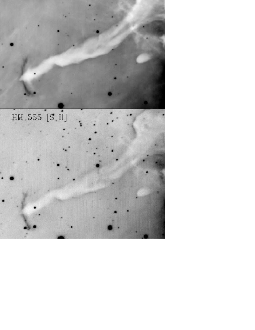
Figure 1: A H$\alpha$ and a red [S II] image of HH 555 taken from Bally & Reipurth (2003).

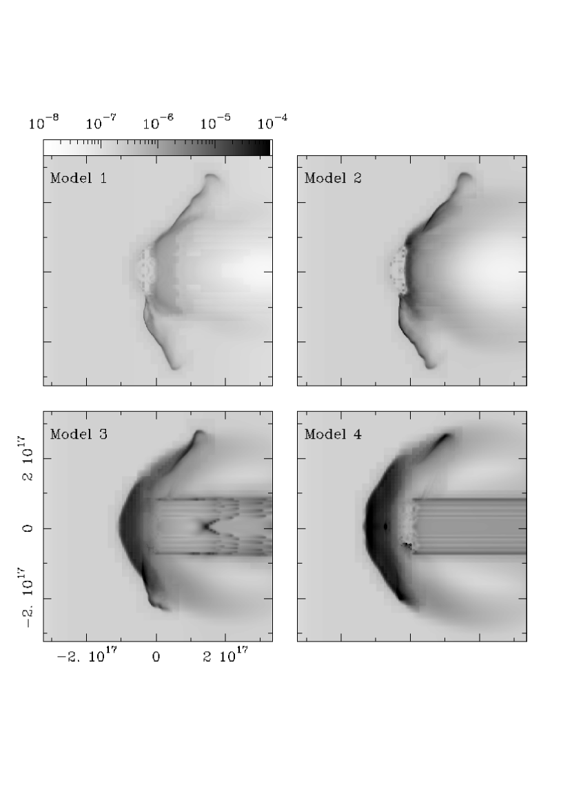
Figure 4: H$\alpha$ emission maps obtained by integrating the H$\alpha$ emission coefficient along the $y$-axis. The extinction within the elephant trunk was not considered. The emission is depicted with the logarithmic greyscale shown by the top bar, in units of erg s^-1 cm^-2 sterad^-1. For the details of the models, see Figure 2 and §3. The axes are labeled in cm.

References

- (1) Bally, J., O’Dell, C. R., McCaughrean, M. J., 2000, AJ, 119, 2919
- (2) Bally, J., Reipurth, B., 2001, ApJ, 546, 299
- (3) Bally, J., Reipurth, B., 2003, AJ, 126, 893
- (4) Cantó, J, Raga, A. C., 1995, MNRAS, 277, 1120
- (5) Cantó, J., Raga, A. C., Steffen, W., Shapiro, P. 1998, ApJ, 502, 695
- (6) Henney, W. J, Raga, A. C., Lizano, S., Curiel, S., 1996, ApJ, 465, 21
- (7) Lebedev, S. V., Ampleford, D., Ciardi, A., Bland, S. N., Chittenden, J. P., Haines, M. G.; Frank, A., Blackman, E. G., Cunningham, A., 2004, ApJ, 616, 988
- (8) Masciadri, E., Raga, A. C., 2001, AJ, 121, 408
- (9) Masciadri, E., Raga, A. C., 2004, ApJ, 615, 850
- (10) Mellema, G., Raga, A. C., Cantó, J., Lundqvist, P., Balick, B., Steffen, W., Noriega-Crespo, A., 1998, A&A, 331, 335
- (11) Raga, A. C., Navarro-Gonzáles, R., Villagrán-Muniz, M., 2000, RMxAA, 36, 67
- (12) Raga, A. C., Reipurth, B., 2004, RMxAA, 40, 15
- (13) Raga, A. C., Steffen, W., González, R. F., 2005, RMxAA, 41, 45
- (14) Reipurth, B., Yu, K. C., Moriarty-Scheven, G., Bally, J., Aspin, C., Heathcoke, S., 2004, AJ, 127, 1069
- (15) Walawender, J., Bally, J., Reipurth, B., 2005, AJ, 129, 2308