Propagation of coherent waves in elastically scattering media

Abstract

A general method for calculating statistical properties of speckle patterns of coherent waves propagating in disordered media is developed. It allows one to calculate speckle pattern correlations in space, as well as their sensitivity to external parameters. This method, which is similar to the Boltzmann-Langevin approach for the calculation of classical fluctuations, applies for a wide range of systems: From cases where the ray propagation is diffusive to the regime where the rays experience only small angle scattering. The latter case comprises the regime of directed waves where rays propagate ballistically in space while their directions diffuse. We demonstrate the applicability of the method by calculating the correlation function of the wave intensity and its sensitivity to the wave frequency and the angle of incidence of the incoming wave.

I Introduction

Characterization of statistical properties of coherent waves propagating through an elastically scattering disordered medium is relevant for a variety of physical situations, ranging from propagation of electromagnetic waves through interstellar space or the atmosphere, seismology, and medical imaging by ultrasound or light, to electron transport in disordered conductors. When coherent waves propagate through such media their intensity exhibits random, sample-specific, fluctuations known as speckles. These fluctuations result from the interference of rays traveling along different paths. In this article we study the statistics of speckles.

The problem can be characterized by several length scales: The propagation distance of the ray through the medium, $Z$, the elastic mean free path, $\ell$, which is the typical distance the ray travels between two scattering events, and the transport mean free path, $\ell_{tr}$ which characterizes the typical distance for backscattering. In the limit of very thin sample, $Z<\ell$, rays move almost ballistically through the sample, since scattering porbability is small. This regime has been extensively studied Goodman . In the opposite limit of a very wide sample, $Z\gg\ell_{tr}$, the rays propagate diffusively in the system. This regime has been considered in Refs. ZyuzinSpivak, ; KaneLee, ; ZyuzinSpivakRev, . At spatial scales exceeding the transport mean free path the statistical properties of speckles in the diffusive regime (excluding features associated with rare events) are characterized by the diffusion coefficient and are independent of the details of the disorder. The crossover between the ballistic and the diffusive regimes depends, in general, on the features of the disorder. However, when the typical deflection angle for a single scattering is small, and therefore the transport mean free path $\ell_{tr}$ is much larger than the mean free path $\ell$, a third regime emerges. This regime, known as the directed waves regime, is realized when the sample width is much smaller than the transport mean free path while it is much larger than the elastic mean free path, $\ell_{tr}\gg Z\gg\ell$. In this case, the rays experience many small angle scattering events which result in a diffusive dynamics of the ray direction. The total change in propagation direction, however, remains small.

The focus of our study is on directed waves which are important for many applications ranging from laser communications in atmosphere to propagation of acoustic or electromagnetic waves through biological tissues. Similarly to the ballistic and the diffusive regimes, the directed waves regime has also been studied in many papers (see for example Refs. Tatarski, ; Kravtsov, ; Prokhorov, ; Dashen, and references therein). However, our results, in many respects, differ substantially from those obtained in previous studies. One of the main differences is the slow power law decay of the intensity correlation function in space, and the change of its sign, see Fig. 1. This difference affects interpretation of any wave intensity measurement which uses a finite aperture apparatus.

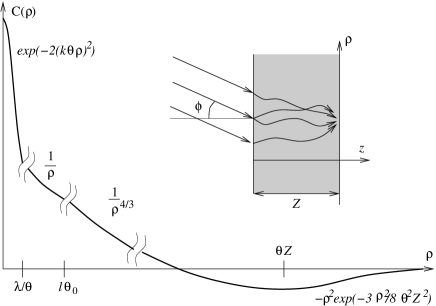
Figure 1: The asymptotic behavior of the intensity correlation function, ${\cal C}(\rho)$, in the directed waves regime. $\rho$ is the distance between the observation points, $\lambda$ is the light wavelength, $\ell$ is the elastic mean free path, $Z$ is the slab width, and $\theta_{0}$ and $\theta$ are the typical scattering angle of a ray traveling a distance $\ell$ and $Z$ respectively.

In this article we develop a general method for calculating speckle correlations over distances larger than the light wavelength, $\lambda$. This method, which is similar (but not identical) to the Langevin scheme for the description of classical fluctuations LandauLifshitz ; ShulmanKogan ; KoganBook , enables one to treat both the diffusive and the directed wave regimes on equal footing. We apply the method to the case of directed waves to evaluate speckle correlations and their sensitivity to various perturbations, such as a change in the frequency of the wave, a variation of the incidence angle, or a change of the refraction index. A short version of these results was published in Ref. Agam2006, .

The paper is organized as follows. In section II.1 we present the general method describing speckle statistics. In sections II.2 and II.3 we consider its limiting cases for angular and spatial diffusion. The treatment of sensitivity of speckle patterns to changes in external parameters is presented in section II.4. In section III we apply our formalism to study speckle correlations in the directed wave regime, and spatial diffusion. Finally, in section IV we present our conclusions. The derivation of the formalism is deferred to the Appendices.

II Methods of description of speckle statistics

A paradigm model for propagation of coherent waves through disordered media is the stationary wave equation for a scalar field $\psi({\bf r})$,

$$k^{2}n^{2}({\bf r})\psi({\bf r})+\nabla^{2}\psi({\bf r})=0,$$ (1)

where $k=2\pi/\lambda$ is the wave number, and $n({\bf r})=1+\delta n({\bf r})$ is the index of refraction. For simplicity we assume $\delta n({\bf r})$ to be a random Gaussian quantity characterized by zero average, and isotropic correlation function

$$\langle\delta n({\bf r})\delta n({\bf r^{\prime}})\rangle=g(|{\bf r-r^{\prime}}|).$$ (2)

Here the angular brackets $\langle\ldots\rangle$ denote averaging over the random realizations of $n({\bf r})$. We assume that the isotropic function $g(r)$ is characterized by a single correlation length, $\xi=[\int d^{3}rr^{2}g(r)/3\int d^{3}rg(r)]^{1/2}$.

The above model is studied below. The central object of our approach is the ray distribution function,

$$f({\bf r},{\bf s})\!=\!\int\!\!\frac{p^{2}dp}{2\pi^{2}}\int\!\!d\mbox{\boldmath$r$}^{\prime}\psi\left({\bf r}\!-\!\frac{{\bf r^{\prime}}}{2}\right)\psi^{*}\left({\bf r}\!+\!\frac{{\bf r^{\prime}}}{2}\right)e^{ip{\bf s}\cdot{\bf r^{\prime}}},$$ (3)

which may be viewed as the density of rays at the point ${\bf r}$ and time $t$ propagating in the direction specified by the unit vector ${\bf s}$. In particular the intensity of the wave at the point ${\bf r}$ is $I({\bf r})\equiv|\psi({\bf r})|^{2}=\int d^{2}sf({\bf r,s})$.

The ray distribution function $f({\bf r,s})$ is a random, sample specific quantity whose statistics can be characterized by its moments. We focus on the first $\langle f({\bf r,s})\rangle$ and second $\langle f({\bf r,s})f({\bf r^{\prime},s^{\prime}})\rangle$ moments of this quantity. These moments quantify the main features of speckle patterns.

II.1 General approach to speckle statistics

In this subsection we discuss a general approach to describe speckles of coherent waves that is valid both in the ballistic and diffusive regimes, and holds for a general angular dependence of the scattering amplitude at a single scatterer.

A general method for calculating moments of the ray distribution function is the disorder diagram technique Abrikosov . If $\ell\gg\lambda$, and on the length scale $|{\bf r-r^{\prime}}|>\lambda$, this formalism can be reduced to a set of equations for the average distribution function, $\langle f({\bf r,s})\rangle$, and the correlation function of the ray distribution function fluctuations, $\langle\delta f({\bf r,s})\delta f({\bf r^{\prime},s^{\prime}})\rangle$, where $\delta f-f-\langle f\rangle$. These equations describe speckles on various length scales: From the ballistic regime to the diffusive limit, and are similar, but not identical, to the Boltzmann-Langevin equations in the kinetic theory of classical particlesShulmanKogan ; KoganBook ; GurevichGanzevichKatilus . Thus $\langle f({\bf r,s})\rangle$ and $\langle\delta f({\bf r,s})\delta f({\bf r^{\prime},s^{\prime}})\rangle$ can be deduced from the following set of equations:

$${\bf s}\cdot\frac{\partial\langle f({\bf r,s})\rangle}{\partial{\bf r}}=I_{st}[\langle f({\bf r,s})\rangle]\equiv\int d^{2}s^{\prime}W({\bf s-s^{\prime}})\left(\langle f({\bf r},{\bf s}^{\prime})\rangle-\langle f({\bf r},{\bf s})\rangle\right),$$ (4)

$${\bf s}\cdot\frac{\partial\delta f({\bf r,s})}{\partial{\bf r}}-I_{st}\{\delta f({\bf r,s})\}={\cal L}({\bf r},{\bf s}),$$ (5)

where the integral over the ray directions, ${\bf s}$, is normalized to unity, $\int d^{2}s=1$, and the Langevin sources, ${\cal L}({\bf r},{\bf s})$, have zero mean and correlations of the form:

$$\langle{\cal L}({\bf r},{\bf s}){\cal L}({\bf r^{\prime}},{\bf s^{\prime}})\rangle=\frac{2\pi}{k^{2}}\,\delta({\bf r}\!-{\bf r^{\prime}})\left[\delta({\bf s}\!-\!{\bf s^{\prime}})\langle f({\bf r,s})\rangle\int d^{2}\tilde{s}W({\bf s}\!-\!\tilde{\bf s})\langle f({\bf r},\tilde{\bf s})\rangle-\langle f({\bf r,s})\rangle W({\bf s}\!-\!{\bf s^{\prime}})\langle f({\bf r},{\bf s^{\prime}})\rangle\right].$$ (6)

Here $W({\bf s-s^{\prime}})$ is the probability, per unit length, for scattering between propagation directions ${\bf s}$ and ${\bf s}^{\prime}$. The mean free path $\ell$ and the transport mean free path $\ell_{tr}$ are expressed in terms of $W({\bf s-s^{\prime}})$ as

$$\ell^{-1} = \int d\mbox{\boldmath$s$}^{\prime}W(\mbox{\boldmath$s$}-\mbox{\boldmath$s$}^{\prime}),\quad\ell_{tr}^{-1}=\int d\mbox{\boldmath$s$}^{\prime}(1-\mbox{\boldmath$s$}\cdot\mbox{\boldmath$s$}^{\prime})W(\mbox{\boldmath$s$}-\mbox{\boldmath$s$}^{\prime}).$$ (7)

In the Born approximation the scattering probability can be expressed in terms of the refraction index correlator, Eq. (2), as

$$W({\bf s})=\frac{k^{4}}{\pi}\int d^{3}rg({\bf r})e^{ik{\bf s}\cdot{\bf r}}.$$ (8)

The derivation of Eqs. (4-6), using the standard impurity diagram technique Abrikosov , is presented in Appendix A. On spatial scales larger than $\ell$, and $\ell_{tr}$ it is possible to simplify Eqs. (4-6) reducing them to a diffusion-type equations. Another simplification occurs if the scattering angle at a single impurity is small. Then at lengths greater than the mean free path the change of direction of the wave propagation is described by diffusion in the angular space. The simplified form of the general formalism in these two limits is considered in Sections II.2 and II.3.

Qualitatively the form of the correlation function of the random sources, Eq. (6), can be understood as follows. Inside the random medium the propagating wave can be viewed as a random superposition of plane waves arriving from different directions. The relative phases of the different plane waves are uncorrelated. Let us consider scattering of this incident wave at a given impurity. Denoting the amplitude of the wave incident in the direction $\bm{s}$ by $i(\bm{s})$ we can express the angular dependence of the the outgoing wave, $o(\bm{s})$, as

$$o(\bm{s})=i(\bm{s})+2ik\int d\bm{s}^{\prime}F(\bm{s},\bm{s}^{\prime})i(\bm{s}^{\prime}),$$

where $F(\bm{s},\bm{s}^{\prime})$ is the scattering amplitude. The intensity of the outgoing wave in the direction $\bm{s}$ is

$$|o(\bm{s})|^{2}=|i(\bm{s})|^{2}-4k\int d\bm{s}^{\prime}\mathrm{Im}\left[F(\bm{s},\bm{s}^{\prime})i^{*}(\bm{s})i(\bm{s}^{\prime})\right]+4k^{2}\left|\int d\bm{s}^{\prime}F(\bm{s},\bm{s}^{\prime})i(\bm{s}^{\prime})\right|^{2}.$$ (9)

The flux into direction $\bm{s}$ due to scattering, $j(\bm{s})=|o(\bm{s})|^{2}-|i(\bm{s})|^{2}$, is a random quantity. Since the amplitudes $i(\bm{s})$ of the incident wave are uncorrelated for different directions, $\langle i(\bm{s})i^{*}(\bm{s}^{\prime})\rangle\sim\delta(\bm{s}-\bm{s}^{\prime})\langle f(\bm{s})\rangle$, the average flux is given by

$$\langle j(\bm{s})\rangle=-4k\langle f(s)\rangle\mathrm{Im}[F(\bm{s},\bm{s})]+4k^{2}\int d\bm{s}^{\prime}|F(\bm{s},\bm{s}^{\prime})|^{2}\langle f(\bm{s}^{\prime})\rangle=4k^{2}\int d\bm{s}^{\prime}|F(\bm{s},\bm{s}^{\prime})|^{2}[\langle f(\bm{s}^{\prime})\rangle-\langle f(\bm{s})\rangle],$$ (10)

in agreement with Eq. (4). The last equality in Eq. (10) follows from the optical theorem, $\mathrm{Im}[F(\bm{s},\bm{s})]=k\int d\bm{s}^{\prime}|F(\bm{s},\bm{s}^{\prime})|^{2}$.

For a specific realization of the incident wave, the flux scattered in direction $\bm{s}$ differs from its average. In the spirit of the Boltzmann-Langevin approach one has to evaluate the fluctuations of microscopic fluxes in the ${\bf s}$ space and substitute them into the kinetic equation as random sources ${\cal L}(\bm{s})\sim j(\bm{s})$, see Eq. (5). Thus, for the correlation function of these quantities, $\langle{\cal L}(\bm{s}){\cal L}(\bm{s}^{\prime})\rangle\sim\langle j(\bm{s})j(\bm{s}^{\prime})\rangle$, and using Eq. (9) one gets the estimate,

$$\langle{\cal L}(\bm{s}){\cal L}(\bm{s}^{\prime})\rangle\sim\delta(\bm{s}-\bm{s^{\prime}})\langle f(\bm{s})\rangle\int d\tilde{\bm{s}}\,|F(\bm{s},\tilde{\bm{s}})|^{2}\langle f(\tilde{\bm{s}})\rangle-\langle f(\bm{s})\rangle\langle f(\bm{s}^{\prime})\rangle|F(\bm{s},\bm{s}^{\prime})|^{2}.$$

in agreement with Eq. (6). Here we took into account the fact that in the limit $\ell\gg\lambda,F(\bm{s},\bm{s}^{\prime})$ the main contribution to the flux correlations comes from the middle term in the right hand side of Eq. (9).

II.1.1 A comparison between Eqs. (4-6) and the Langevin description of classical fluctuations.

It is instructive to compare the method describing classical kinetics of particlesShulmanKogan ; KoganBook ; GurevichGanzevichKatilus with the description of coherent wave propagating through a disordered media expressed by Eqs. (4-6). Consider noninteracting particles propagating in a scattering medium, and let $\tilde{f}({\bf r,s},t)$ denote their distribution function in phase space. The scattering process of the particle is random in time and space. This randomness leads to temporal fluctuations of the distribution function $\tilde{f}$ even when the incident particle flux is stationary. It is, therefore, natural to decompose the distribution function $\tilde{f}({\bf r,s};t)$ into a sum of its average, $\langle\langle\tilde{f}({\bf r,s};t)\rangle\rangle$, and fluctuating part, $\delta\tilde{f}({\bf r,s};t)$, characterized by the correlation function $\langle\langle\delta\tilde{f}\delta\tilde{f}\rangle\rangle$. Here $\langle\langle\cdots\rangle\rangle$ denotes the averaging over time, or over the statistical ensemble clav .

When the elastic mean free path is much larger than the disorder correlation length, $\ell\gg\xi$, The average distribution function satisfies the Boltzmann kinetic equation:

$$\frac{\partial\langle\langle\tilde{f}({\bf r,s},t)\rangle\rangle}{c\,\partial t}+{\bf s}\cdot\frac{\partial\langle\langle\tilde{f}({\bf r,s};t)\rangle\rangle}{\partial{\bf r}}=I_{st}\{\tilde{f}({\bf r,s};t)\}\equiv$$

$$\int d{\bf s}^{\prime}[I_{st}^{(+)}({\bf s,s^{\prime}})+I_{st}^{(-)}({\bf s,s^{\prime}})]=\int d^{2}{\bf s}^{\prime}\,W({\bf s\!-\!{\bf s}^{\prime}})\left(\langle\langle\tilde{f}({\bf r},{\bf s}^{\prime};t)\rangle\rangle-\langle\langle\tilde{f}({\bf r},{\bf s};t)\rangle\rangle\right).$$ (11)

where $c$ is the particle velocity, $I_{st}^{(+)}({\bf s,s^{\prime}})$ denotes the particle flux from $\bm{s}^{\prime}$ to $\bm{s}$ due to collisions, and $I_{st}^{(-)}({\bf s,s^{\prime}})$ denotes the particle flux from $\bm{s}$ to $\bm{s}^{\prime}$,

$$I_{st}^{(+)}({\bf s,s^{\prime}}) = W({\bf s\!-\!\tilde{s}})\tilde{f}({\bf r},{\bf s}^{\prime};t)\left(1\pm\tilde{f}({\bf r},{\bf s};t)\right),$$

$$I_{st}^{(-)}({\bf s,s^{\prime}}) = -W({\bf s-s^{\prime}})\tilde{f}({\bf r},{\bf s},t)\left(1\pm\tilde{f}({\bf r},{\bf s^{\prime}};t)\right).$$

The $\pm$ sings in front of $\tilde{f}({\bf r},{\bf s^{\prime}};t)$ correspond to boson (+) and fermion ($-$) statistics. Notice however that the quadratic terms in $\langle\langle\tilde{f}({\bf r,s},t)\rangle\rangle$ cancel out in the Boltzmann equation (11) and regardless of the particle statistics.

The statistical behavior of the fluctuations of the distribution function, $\delta\tilde{f}({\bf r,s};t)$, may be deduced from the Langevin equation ShulmanKogan ,

$$\frac{\partial\delta\tilde{f}({\bf r,s},t)}{c\,\partial t}+{\bf s}\cdot\frac{\partial\delta\tilde{f}({\bf r,s},t)}{\partial{\bf r}}=I_{st}\{\delta\tilde{f}({\bf r,s})\}+\tilde{I}_{L}({\bf r},t),$$ (12)

where $\tilde{I}_{L}$ represents a random Langevin source with vanishing expectation value and two point correlation function given by

$$\langle\langle\tilde{I}_{L}({\bf r,s},t)\tilde{I}_{L}({\bf r^{\prime},s^{\prime}},t^{\prime})\rangle\rangle=\delta(t\!-\!t^{\prime})\delta({\bf r\!-\!r^{\prime}})\left\{\delta({\bf s-s^{\prime}})\!\int ds^{\prime\prime}[I_{st}^{(+)}({\bf s,s^{\prime\prime}})+I_{st}^{(-)}({\bf s,s^{\prime\prime}})]-[I_{st}^{(+)}({\bf s,s^{\prime}})+I_{st}^{(-)}({\bf s,s^{\prime}})]\right\}.$$ (13)

The classical limit of this equation corresponds to $\langle\langle\tilde{f}({\bf r},{\bf s},t)\rangle\rangle\ll 1$. In this case particle statistics are irrelevant. The description of the evolution of the average ray distribution function, by the Boltzmann kinetic equation of a classical particle holds as long as $\ell\gg\xi,\lambda$. The above formulaes have the following interpretationShulmanKogan ; KoganBook : The scattering processes are instantaneous and local therefore the correlation function of Langevin sources (13) is proportional to $\delta({\bf r-r^{\prime}})\delta(t-t^{\prime})$. Thus scattering events generate correlations of Langevin sources that are nonlocal only in the space of the particle directions. These are described by the four terms in the curly brackets. The first two terms, proportional to $\delta(\bm{s}-\bm{s}^{\prime})$, describe self-correlation generated by flux of particles which scatter from the state $\bm{s}$ to an arbitrary state $\bm{s}^{\prime\prime}$ or vice versa. The two other terms in the curly brackets correspond to scattering events from ${\bf s}$ to ${\bf s^{\prime}}$, or back.

The set of Eqs. (11-13) describing the kinetics of classical particle and that of Eqs. (4-6) describing coherent waves have a similar form. We would like to point out significant differences originating from the different nature of fluctuations. A stationary coherent wave propagating through a disordered sample experiences no temporal fluctuations. In this case the spatial fluctuations of $f({\bf r,s})$ result from the random nature of the interference processes associated with different quasiclassical wave propagation paths. As a result the random sources, Eq. (6), are $\delta$-correlated in space and do not depend on time. In contrast, in the case of classical particles $\tilde{f}$ fluctuates both in space and in time, and consequently the random classical sources, Eqs. (12-13) are $\delta$-correlated both in space and in time.

Another significant difference manifests itself in dramatically different sensitivities of these two phenomena to small changes of parameters, such as particle’s velocities (or wavelength), frequencies, and configuration of the scattering potential. In the case of classical particles the correlators $\langle\langle\tilde{f}\rangle\rangle$ and $\langle\langle\delta\tilde{f}\delta\tilde{f}\rangle\rangle$ are insensitive to these changes as long as the scattering probability $W(\bm{s}-\bm{s}^{\prime})$ does not depend on the wave length or the energy of the particles. In contrast, the coherent speckles exhibit very strong sensitivity to these changes. As a result the form of the correlation functions of the random sources describing these sensitivities, see Eq. (25), is very different from that in Eq. (13).

II.2 Angular diffusion

As mentioned above the solutions of Eqs. (4-6) provide description of $\langle f({\bf r,s})\rangle$ and $\delta\langle f({\bf r,s})\delta f({\bf r^{\prime},s^{\prime}})\rangle$ on the resolution where $|{\bf r-r^{\prime}}|>\lambda$. A simplified description is obtained when the required resolution is over larger length scales. Consider the case $|{\bf r-r^{\prime}}|\gg\ell\theta_{0}$, where $\theta_{0}=\lambda/\xi$ is the typical scattering angle over a distance of the order of the mean free path (notice that the Born approximation implies that $\ell\theta_{0}\gg\lambda$). The reduction of Eqs. (4-6), for this case, is similar in spirit to the standard way by which Boltzmann equation is reduced to the diffusion equation. It follows from the assumption that $f({\bf s,r})$ changes slowly as function of ${\bf s}$ on the scale of order $\theta_{0}$. The resulting formulae, provided below, describe diffusive spreading of the rays in the space of directions, ${\bf s}$. Equation (4) reduces to

$${\bf s}\cdot\frac{\partial\langle f({\bf r,s}\rangle}{\partial{\bf r}}=D_{\theta}\nabla_{s}^{2}\langle f({\bf r,s})\rangle,$$ (14)

where

$$D_{\theta}=\frac{1}{2}\,\ell_{tr}^{-1}$$ (15)

is the diffusion constant in the space of angles, ${\bf s}$, and

$$\nabla_{s}=\hat{\theta}\frac{\partial}{\partial\theta}+\frac{\hat{\phi}}{\sin(\theta)}\frac{\partial}{\partial\phi}$$ (16)

is the gradient operator, with the unit vectors $\hat{\phi}=(-\sin\phi,\cos\phi,0)$ and $\hat{\theta}=(\cos\phi\cos\theta,-\sin\phi\cos\theta,-\sin\phi)$ (here $\theta$ and $\phi$ are the angles associated with polar coordinates).

The fluctuations of the ray distribution function in this case are described by the equation

$${\bf s}\cdot\frac{\partial\delta f({\bf r,s})}{\partial{\bf r}} = \nabla_{s}\left[D_{\theta}\nabla_{s}\delta f({\bf r,s})-{\bf j}^{L}({\bf r},{\bf s})\right],$$ (17)

where the Langevin current sources, ${\bf j}^{L}({\bf r},{\bf s})$, are correlated as

$$\langle j^{L}_{\alpha}({\bf r},{\bf s})j^{L}_{\beta}(\tilde{\bf r},\tilde{\bf s})\rangle = \frac{2\pi D_{\theta}\langle f\rangle^{2}}{k^{2}}\delta_{\alpha\beta}\delta({\bf s}\!-\!\tilde{\bf s})\delta({\bf r}\!-\!\tilde{\bf r}),$$ (19)

where the indices $\alpha$ and $\beta$ denote the vector components in the two-dimensional space of directions that is tangential to the unit sphere $|s|=1$.

II.3 Diffusion in real space

If one is concerned with an even cruder resolution, where $|{\bf r-r^{\prime}}|\gg\ell_{tr}$, the effective description of the system employs the diffusion equation in real space. In this case $f({\bf r,s})$ is assumed to be a nearly isotropic function of ${\bf s}$, and a slow function of $\bm{r}$. Then Eqs. (4-6) can be reduced to the following set of Diffusion-Langevin equations ZyuzinSpivak ; ZyuzinSpivakRev . Namely, expressing the wave intensity, $I(\bm{r})$, at point $\bm{r}$ as $I({\bf r})=\int d^{2}sf(\bm{r},{\bf s})$, one can reduce Eq. (4) to the Laplace equation,

$$\nabla^{2}\langle I({\bf r})\rangle=0,$$ (20)

while the correlator of the intensity fluctuations, $\delta I=I-\langle I\rangle$, can be deduced from the flux conservation condition,

$$\nabla\cdot\delta{\bf J}=0,$$ (21)

with

$$\delta{\bf J}=-D\nabla\delta I+{\bf J}^{L}.$$ (22)

Here $D=\ell_{tr}/3$ is the diffusion constant in real space (notice that according to our convention the diffusion constant has dimensions of length). The Langevin current sources, ${\bf J}^{L}$, have a vanishing expectation value and are characterized by the correlation function:

$$\langle J_{\alpha}^{L}({\bf r})J_{\beta}^{L}({\bf r^{\prime}})\rangle=\frac{\lambda^{2}D}{2\pi}\langle I({\bf r})\rangle^{2}\delta_{\alpha\beta}\delta({\bf r}-{\bf r^{\prime}}).$$ (23)

The boundary conditions for these equations are the conventional conditions for the diffusion equation: $\delta I=0$ at open boundaries, and ${\bf J}\cdot\bm{n}=0$, with $\bm{n}$ being the normal to the boundary, at closed boundaries.

II.4 Sensitivities of speckles to changes of external parameters.

The interfering waves travel along different paths, and the lengths of these paths are much longer than the wave length. Therefore the phases accumulated along each path are very sensitive to changes of external parameters such as the wave number $k$, the incidence angle of the incoming wave, or a smooth change in the refractive index $\Delta n({\bf r})$. We will characterize these changes by the control parameter $\gamma({\bf r})=\Delta k+k\Delta n({\bf r})$ where $\Delta k$ denotes a change in the wave number, $k$. The formalism presented above may be straightforwardly generalized to calculate the sensitivity of the speckle pattern to various external perturbations. The sensitivity of the speckle pattern can be characterized by the correlator of the ray distribution functions at different values of the control parameter, $\langle\delta f({\bf r,s},0)\delta f({\bf r,s},\gamma)\rangle$. In order to evaluate it Eq. (5) should be replaced by two equations. One for $\delta f({\bf r,s},0)$, and another for $\delta f({\bf r,s},\gamma)$. The form of these equations is precisely that of Eq. (5), however the Langevin sources now depend on the perturbation parameter $\gamma$. Namely

$${\bf s}\cdot\frac{\partial\delta f({\bf r,s};\gamma)}{\partial{\bf r}}-I_{st}\{\delta f({\bf r,s};\gamma)\}={\cal L}({\bf r},{\bf s};\gamma),$$ (24)

where ${\cal L}({\bf r},{\bf s};\gamma)$ denotes the Langevin source associated with the value $\gamma$ of the perturbation. The average of the Langevin sources vanishes. Their correlation function, at different points in space and different values of the control parameter, is given by

$$\langle{\cal L}({\bf r},{\bf s};0){\cal L}({\bf r^{\prime}},{\bf s^{\prime}};\gamma)\rangle\!=\!\frac{\pi}{k^{2}}\delta({\bf r}\!-{\bf r^{\prime}})\sum_{\nu=\pm}\left[\delta({\bf s}\!-\!{\bf s^{\prime}})f_{\nu}({\bf r,s})\int d^{2}{\bf s}_{1}W({\bf s}\!-\!{\bf s}_{1})f_{-\nu}({\bf r},{\bf s}_{1})-f_{\nu}({\bf r},{\bf s})W({\bf s}\!-\!{\bf s^{\prime}})f_{-\nu}({\bf r},{\bf s^{\prime}})\right],$$ (25)

where $f_{\pm}({\bf r,s})$ satisfies the equation,

$${\bf s}\cdot\frac{\partial f_{\pm}({\bf r,s})}{\partial{\bf r}}-I_{st}\{f_{\pm}({\bf r,s})\}=\pm i\gamma f_{\pm}({\bf r,s}).$$ (26)

At free boundaries, the boundary conditions for the functions $f_{\pm}({\bf r,s})$ coincide with the standard boundary conditions for the Boltzmann equation. At the boundary with an incident radiation, denoted by ${\cal S}$, the functions $f_{\pm}({\bf r,s})$ are determined by the parametric correlations in the incident wave, i.e.

$$\left.f_{+}({\bf r},{\bf s})\right|_{\bm{r}\in{\cal S}}\!=\!\int\!\!\frac{p^{2}dp}{2\pi^{2}}\int\!\!d\mbox{\boldmath$r$}^{\prime}\psi_{\gamma}\left({\bf r}\!-\!\frac{{\bf r^{\prime}}}{2}\right)\psi_{0}^{*}\left({\bf r}\!+\!\frac{{\bf r^{\prime}}}{2}\right)e^{ip{\bf s}\cdot{\bf r^{\prime}}}.$$ (27)

Here the subscript of the wave amplitude $\psi$ denotes the value of the parameter $\gamma$. The corresponding equation for $f_{-}({\bf r},{\bf s})$ is obtained from Eq. (27) by interchanging the subscripts: $\gamma\leftrightarrow 0$.

When the external perturbation is associated with a change in the incidence angle of the incoming wave, Eq. (25) still holds, however, both $f_{+}({\bf r,s})$ and $f_{-}({\bf r,s})$ satisfy the same equation (14). The difference between $f_{+}({\bf r,s})$ and $f_{-}({\bf r,s})$ arise from the boundary conditions,(27). We shall elaborate on this issue in Section III.1.2.

The above formulae describe the speckle sensitivity on the resolution scale larger than the wavelength. As discussed in the previous section the formalism simplifies for lower resolution. We conclude this section by providing the relevant formulas for the case of angular diffusion, and diffusion is real space.

II.4.1 Sensitivity in the case of angle diffusion

If the typical scattering angle at a single impurity is small and wave propagation length exceeds the mean free path, $\ell$, the equation for the fluctuations in the ray distribution function is

$${\bf s}\cdot\frac{\partial\delta f({\bf r,s};\gamma)}{\partial{\bf r}} = \nabla_{s}\left[D_{\theta}\nabla_{s}\delta f({\bf r,s};\gamma)-{\bf j}^{L}({\bf r},{\bf s};\gamma)\right],$$ (28)

where the Langevin current sources, ${\bf j}^{L}({\bf r},{\bf s};\gamma)$ depend on the perturbation $\gamma$. These have zero mean and correlation function given by

$$\langle j^{L}_{\alpha}({\bf r},{\bf s};0)j^{L}_{\beta}(\tilde{\bf r},\tilde{\bf s};\gamma)\rangle = \frac{2\pi D_{\theta}f_{+}({\bf r},{\bf s})f_{-}({\bf r},{\bf s})}{k^{2}}\delta_{\alpha\beta}\delta({\bf s}\!-\!\tilde{\bf s})\delta({\bf r}\!-\!\tilde{\bf r}),$$ (29)

where $f_{\pm}({\bf r},{\bf s})$ satisfy the equation

$${\bf s}\cdot\frac{\partial f_{\pm}({\bf r,s})}{\partial{\bf r}}=D_{\theta}\nabla_{s}^{2}f_{\pm}({\bf r,s})\pm i\gamma f_{\pm}({\bf r,s}).$$ (30)

II.4.2 Sensitivity in the case of the real space diffusion

Finally, on spatial scale larger than the transport mean free path $\ell_{tr}$, the sensitivity of the speckle pattern may be described by the current conservation condition,

$$\nabla\cdot\delta{\bf J}=\nabla\cdot\left(-D\nabla\delta I+{\bf J}^{L}\right)=0,$$ (31)

where the Langevin current sources, at different values of the perturbation parameter, $\gamma$, are correlated as

$$\langle J_{\alpha}^{L}({\bf r};0)J_{\beta}^{L}({\bf r^{\prime}};\gamma)\rangle=\frac{\lambda^{2}D}{2\pi}I_{+}({\bf r})I_{-}({\bf r})\delta_{\alpha\beta}\delta({\bf r}-{\bf r^{\prime}}),$$ (32)

and $I_{\pm}({\bf r})$ satisfies the equation

$$D\nabla^{2}I_{\pm}({\bf r})\pm i\gamma I_{\pm}({\bf r})=0.$$ (33)

III Evaluation of speckle correlation functions and speckle sensitivities to changes of external parameters

In this section we shall illustrate the use of the formalism developed in the previous section. To this end we will consider the correlation function of speckles and their sensitivity to various perturbations in the regimes of directed waves as well as for diffusion in real space.

III.1 Speckles in the regime of directed waves

Consider a situation in which a wave of intensity $I_{0}$ is incident on a disordered slab of thickness $Z$, as shown in the inset of Fig. 1. The slab thickness is assumed to be much smaller than the transport mean free path and much larger than the elastic mean free path, $\ell_{tr}\gg Z\gg\ell$. Thus rays diffuse in angle, but their total change of direction is small. In this regime of directed waves it will be convenient to choose the coordinate system ${\bf r}=(\mbox{\boldmath$\rho$},z)$ where $z$ is the the direction of the wave propagation in the absence of disorder ($\delta n({\bf r})=0$), and $\rho$ denotes a two dimensional vector in the plane perpendicular to the $z$-axis. Similarly we decompose the vector of the ray direction as ${\bf s}=({\bf s}_{\perp}),s_{z}$, where $s_{z}$ denotes the component in the $z$ direction, while ${\bf s}_{\perp}$ is a two dimensional vector in the perpendicular plane. The rays of directed waves are almost parallel to the $z$ axis and therefore $s_{z}\approx 1$, i.e. ${\bf s}\approx({\bf s}_{\perp},1)$. If we denote by $\theta$ the typical ray angle at $z=Z$, then the latter approximation holds as long as $\theta\ll 1$. The results which we present below are calculated to leading order in the small parameter $\theta$.

It is instructive to start with understanding the classical evolution of the average ray distribution function in the regime of directed waves. For this purpose we solve Eq. (14) for the case where a single ray moving in the $z$ direction, impinges upon the slab at the origin ${\bf r}=0$. The assumption that ${\bf s}\simeq({\bf s}_{\perp},1)$ allows one to reduce Eq. (14) to

$$\frac{\partial\langle f({\bf r,s})\rangle}{\partial z}+{\bf s}_{\perp}\cdot\frac{\partial\langle f({\bf r,s})\rangle}{\partial\mbox{\boldmath$\rho$}}-D_{\theta}\frac{\partial^{2}\langle f({\bf r,s})\rangle}{\partial{\bf s}_{\perp}^{2}}=0.$$ (34)

The boundary conditions are

$$\left.\langle f({\bf r},{\bf s})\rangle\right|_{z=0}=i_{0}\delta(\mbox{\boldmath$\rho$})\delta({\bf s}_{\perp}),$$ (35)

where the amplitude $i_{0}$ denotes the incident ray intensity. The solution of the above problem takes the form

$$\langle f({\bf r},{\bf s})\rangle=\frac{3i_{0}}{4\pi^{2}D_{\theta}^{2}z^{4}}\exp\left[-\frac{3\mbox{\boldmath$\rho$}^{2}}{D_{\theta}z^{3}}+\frac{3{\bf s}_{\perp}\mbox{\boldmath$\rho$}}{D_{\theta}z^{2}}-\frac{{\bf s}_{\perp}^{2}}{D_{\theta}z}\right].$$ (36)

It demonstrates the diffusive behavior of the ray direction as it propagates in the slab, $|{\bf s}_{\perp}|^{2}\sim D_{\theta}z$. It also shows that deviations in real space grow in a superdiffusive mannerJayannavar82 , $\rho^{2}\sim D_{\theta}z^{3}$.

After this preliminary consideration we turn to study intensity correlations of directed waves. To be specific we consider a plane wave (not restricted by a finite aperture) incident on the disordered slab in the $z$-direction. In this case the average ray distribution function is independent of the perpendicular coordinate $\bm{\rho}$ and can be easily obtained by integrating Eq. (36) over $\bm{\rho}$,

$$\langle f(z,{\bf s})\rangle=\frac{i_{0}}{4\pi D_{\theta}z}\exp\left[-\frac{{\bf s}_{\perp}^{2}}{4D_{\theta}z}\right].$$ (37)

The intensity correlation function,

$${\cal C}(\delta{\bf r})\equiv\langle\delta I({\bf r})\delta I({\bf r}+\delta\bm{r})\rangle,$$ (38)

where $\delta I({\bf r}=I({\bf r})-\langle I({\bf r}\rangle$, is independent of the transverse coordinate and depends only on the propagation distance $Z$ and the difference coordinate $\delta\bm{r}$. The behavior of this correlator as a function of $\delta\bm{r}=(\bm{\rho},\delta z)$ is strongly anisotropic. Consider first the case where the observation points are located along the $z$ axis (i.e. $\bm{\rho}=\bf{0}$) near the point $z=Z$. In this case we obtain

$${\cal C}(\delta z)=\frac{I_{0}^{2}}{4k^{2}\theta^{4}\delta z^{2}},$$ (39)

where $\theta=\sqrt{D_{\theta}Z}$ is the accumulated scattering angle, and the condition $\ell\ll\delta z\ll Z$ is assumed. This formula, which also approximates the behavior for nonzero $\rho$ as long as $\delta z\gg\rho/\theta$, matches the results for the diffusive case ZyuzinSpivak ; ZyuzinSpivakRev , $Z\gg\ell_{tr}$ when $\theta$ is of order unity.

A more complex behavior of the correlation function appears when $\delta z<\rho/\theta$, i.e. when the observation points are located essentially in the plane perpendicular to the $z$-axis. A general formula for ${\cal C}(\mbox{\boldmath$\rho$})$, in this case, is derived in Appendix B. The expression takes the form

$${\cal C}(\rho) = \frac{I_{0}^{2}}{4D_{\theta}k^{2}}\int_{0}^{Z-\ell}\!\frac{d\zeta}{\zeta-Z}\int_{0}^{\infty}\!\!dqqJ_{0}(q\rho)\frac{d}{d\zeta}\exp\left[-\frac{2}{\ell}\int_{0}^{\zeta}d\eta\left\{1-\tilde{g}\left(\frac{q}{k}\eta\right)\right\}\right],$$ (40)

where $\tilde{g}(\rho)=\int dzg(\sqrt{\rho^{2}+z^{2}})/\int dzg(z)$, and $J_{0}(x)$ is the Bessel function of zeroth order.

The integral in Eq. (40) contains a term proportional to a $\delta$-function, $\frac{\pi I_{0}^{2}}{2D_{\theta}k^{2}Z}\delta(\mbox{\boldmath$\rho$})$. This term represents the rapidly decaying (at $\rho\sim\lambda/\theta$) part of the correlator. It results from the semiclassical approximation employed in the derivation of Eqs. (4-6), which limits the spacial resolution to $\rho>\lambda$. In order to resolve the spatial structure on smaller scales some of the diagrams discussed in Appendix A should be calculated more accurately. The result of this calculation shows that the $\delta$ function contribution to the correlator ${\cal C}(\rho)$ is in fact a contribution of the form $I_{0}^{2}e^{-2(k\theta\rho)^{2}}$ where $\theta^{2}=D_{\theta}Z$.

As we show below, ${\cal C}(\rho)$ contains also a slowly decaying term. The latter, which has been overlooked in previous studies, clearly has important consequences. In order to understand this term it will be instructive to explain, first, the origin of the short ranged contribution to ${\cal C}(\rho)$. As we show now, it arises from a superposition of statistically independent contributions of waves moving in all possible directions. Let us assume that wave function at a given point on the screen is a sum of plane waves. The distribution of directions of these plane waves is dictated by the diffusive nature of the rays in the system, thus

$$\psi(\mbox{\boldmath$\rho$})=\sum_{\nu}A_{\nu}e^{ik{\bf s}_{\perp,\nu}\cdot\mbox{\boldmath$\rho$}}$$ (41)

where ${\bf s}_{\perp,\nu}$ denotes the direction of the $\nu$-th contribution and $A_{\nu}$ is the corresponding amplitude. We shall assume that $A_{\nu}$ are statistically independent variables, with zero mean and fluctuation strength given by

$$\langle|A_{\nu}|^{2}\rangle=\frac{I_{0}}{4\pi D_{\theta}Z}e^{\frac{|{\bf s}_{\perp,\nu}|^{2}}{4D_{\theta}Z}}.$$ (42)

The average $\langle|A_{\nu}|^{2}\rangle$ may be interpreted as the “classical” probability to find a plain wave moving in direction ${\bf s}_{\perp,\nu}$. It may be obtained from the solution of Eq. (34) with boundary conditions which correspond to an impinging plane wave of density $I_{0}$, $\left.\langle f({\bf r},{\bf s})\rangle\right|_{z=0}=I_{0}\delta({\bf s}_{\perp})$.

The above assumptions imply that, at a given point in space, $\psi(\mbox{\boldmath$\rho$})$ is approximately a Gaussian random variable, as a result of the central limit theorem. Moreover, the wave function at two different points, $\psi(\mbox{\boldmath$\rho$})$ and $\psi(\mbox{\boldmath$\rho$}^{\prime})$, are also described by a joint Gaussian distribution function provided the distance between these points is sufficiently small such that one may assume that the same set of wavelets arrive to both points.

Assuming the observation points $\rho$ and $\mbox{\boldmath$\rho$}^{\prime}$ to be sufficiently close to each other, consider the ensemble average $\langle I(\mbox{\boldmath$\rho$})I(\mbox{\boldmath$\rho$}^{\prime})\rangle=\langle\psi(\mbox{\boldmath$\rho$})\psi^{*}(\mbox{\boldmath$\rho$})\psi(\mbox{\boldmath$\rho$}^{\prime})\psi^{*}(\mbox{\boldmath$\rho$}^{\prime})\rangle$. Using the fact that within a small vicinity of space, $\psi^{*}(\mbox{\boldmath$\rho$})$ may be considered as a random Gaussian function, one deduces that $\langle\psi(\mbox{\boldmath$\rho$})\psi^{*}(\mbox{\boldmath$\rho$})\rangle\langle\psi(\mbox{\boldmath$\rho$}^{\prime})\psi^{*}(\mbox{\boldmath$\rho$}^{\prime})\rangle+\langle\psi(\mbox{\boldmath$\rho$})\psi^{*}(\mbox{\boldmath$\rho$}^{\prime})\rangle\langle\psi(\mbox{\boldmath$\rho$}^{\prime})\psi^{*}(\mbox{\boldmath$\rho$})\rangle$, and hence the density correlation function is given by

$${\cal C}(\mbox{\boldmath$\rho$}-\mbox{\boldmath$\rho$}^{\prime})=\left|\langle\psi(\mbox{\boldmath$\rho$})\psi^{*}(\mbox{\boldmath$\rho$}^{\prime})\rangle\right|^{2}$$ (43)

Now from (41) and the statistical independence of the amplitudes $A_{\nu}$ we see that

$$\langle\psi(\mbox{\boldmath$\rho$})\psi^{*}(\mbox{\boldmath$\rho$}^{\prime})\rangle=\left\langle\sum_{\nu,\nu^{\prime}}A_{\nu}A^{*}_{\nu^{\prime}}e^{ik\left({\bf s}_{\perp,\nu}\mbox{\boldmath$\rho$}-{\bf s}_{\perp,\nu^{\prime}}\mbox{\boldmath$\rho$}^{\prime})\right)}\right\rangle=\sum_{\nu}\langle|A_{\nu}|^{2}\rangle e^{ik{\bf s}_{\perp,\nu}\left(\mbox{\boldmath$\rho$}-\mbox{\boldmath$\rho$}^{\prime}\right)}.$$ (44)

The replacement of the above double sum by a sum over one index is equivalent to the assumption that the interference terms of different amplitudes average out to zero. This traditional procedure in semiclassical analysis, known as the “diagonal approximation” leaves only the classical contribution. Thus substituting (42) in (44) and replacing the sum over $\nu$ by an integral over ${\bf s}_{\perp}$ we obtain an expression for $\langle\psi(\mbox{\boldmath$\rho$})\psi^{*}(\mbox{\boldmath$\rho$}^{\prime})\rangle$, and from (43) we conclude that

$${\cal C}(\mbox{\boldmath$\rho$}-\mbox{\boldmath$\rho$}^{\prime})\approx I_{0}^{2}e^{-2(k\theta|\mbox{\boldmath$\rho$}-\mbox{\boldmath$\rho^{\prime}$}|)^{2}}.$$ (45)

This expression, which shows very fast decay of correlations on a scale of order $\lambda/\theta$, has rather limited range of applicability. The reason is that the description of the wave function in the sample, using the superposition of independent plane waves (41), gives reasonable approximation only when the observation points are very close. At larger distances diffraction and quantum impurity scattering give rise to correlation of rays which manifest themselves in a slow decay of the intensity correlations, as well a change of sign. These effects are described by Eq. 40, and illustrated in Fig. 1. At various spatial separations $\bm{\rho}$ one can obtain the following asymptotic expressions for the intensity correlator:

$$\frac{{\cal C}(\rho)}{I_{0}^{2}}\approx\left\{\begin{array}[]{ll}e^{-2(k\theta\rho)^{2}}&\textrm{if~{}~{}~{} $\rho\sim\alpha\lambda/\theta$},\\ \frac{b_{1}}{k^{2}\theta^{2}\ell\theta_{0}\rho}&\textrm{if~{}~{}~{} $\alpha\lambda/\theta\ll\rho\ll\ell\theta_{0}$},\\ \frac{b_{2}D_{\theta}^{2/3}}{k^{2}\theta^{4}\rho^{4/3}}&\textrm{if~{}~{}~{} $\ell\theta_{0}\ll\rho\ll\theta Z$},\\ \frac{-b_{3}\rho^{2}}{k^{2}\theta^{6}Z^{4}}e^{-\frac{3\rho^{2}}{8\theta^{2}Z^{2}}}&\textrm{if~{}~{}~{} $\theta Z\ll\rho\ll\frac{Z\theta^{2}}{\theta_{0}}$},\end{array}\right.$$ (46)

where $\alpha^{2}=\log(k\ell\theta^{3}/\theta_{0})$, $b_{1}=\int_{0}^{\infty}dx\tilde{g}(x)/\xi$ is a constant of order unity, $b_{2}=3^{1/3}\Gamma(5/3)/8\approx 0.163$, and $b_{3}=27/128\approx 0.21$. The qualitative form of the function ${\cal C}(\rho)$ is shown in Fig. 1.

In order to clarify the connection between ray diffraction and the slow decay of the density correlations, let us focus on the regime $\ell\theta_{0}\ll\rho\ll\theta Z$. Consider two points separated by a distance $\rho$. The correlations of the wave intensity in these points emerge from coherent waves which simultaneously arrive to the two points. These can be generated by diffraction which acts as a beam splitter, and modeled by the Langevin sources in Eq. (5). Now, the superdiffusion nature of the ray dynamics in the sample implies that the relevant points where diffraction takes place should be located at distance of order $\Delta z$ from the screen, where $\rho^{2}=D_{\theta}\Delta z^{3}$. The wave intensity emitted from these diffraction points decays as $1/\Delta z^{2}$, and therefore the correlations which they generate are proportional to $D_{\theta}^{2/3}/\rho^{4/3}$.

The above crude argument explains the power law decay of ${\cal C}(\rho)$, in the regime $\ell\theta_{0}\ll\rho\ll\theta Z$. Yet a closer examination of the integrals leading to this results shows that the contribution from diffraction points (or Langevin sources) that are closer to the screen than, $\Delta z=(D_{\theta}\rho^{2})^{1/3}$ generate anti-correlations, while those that are at larger distances provide positive correlations. This behavior may be expected since diffraction points located too close to the screen generate rays which may arrive to either one of the observation points but not to both of them, therefore they lead to anti-correlated behavior. On the other hand, coherent waves generated by diffraction that took place at distances larger than $\Delta z$, get, in general, to both points, and therefore generate positive correlations.

From this picture, and the finite width of the slab, it follows that for sufficiently large distance between the observation points, $\rho^{2}\gg D_{\theta}Z^{3}=(Z\theta)^{2}$, diffraction events can generate only anticorrelations. Thus ${\cal C}(\rho)$ must experience a sign change in the vicinity of $\rho=\theta Z$.

Finally, we mention that the tail of the correlation function (the regime $\rho>Z\theta^{2}/\theta_{0}$) is also described by Eq. (40). However, it depends on the precise form of the disorder correlation $g(r)$, since this limit is dominated by rare scattering events.

The power law nature of the density correlations of directed waves have important consequences regarding the statistics of the signal measured by sensors with large apertures compared to the wave length. Let

$$P=\int d^{2}\rho d^{2}s~{}{\bf n}\cdot{\bf s}f({\bf r,s}),$$ (47)

denote the signal measured by the sensor, where ${\bf n}$ is a unit vector perpendicular to the sensor surface, and $\rho$ is a two dimensional vector which parameterizes the sensor surface. If the sensor aperture is circular, with radius $R$, and its surface is perpendicular to the propagation direction, i.e. ${\bf s\cdot n}\sim 1$, then the integrated power measured by the sensor may be approximated by an integral over the wave density

$$P(R)=\int_{|\mbox{\boldmath$\rho$}|<R}d^{2}\rho I({\bf r}),$$ (48)

where ${\bf r}=(\mbox{\boldmath$\rho$},z)$. The random fluctuations of $I({\bf r})$ imply that $P(R)$ is also a random quantity. Its average may be expressed as an integral over $\langle I({\bf r})\rangle$, while the variance of its fluctuations is given by

$$\langle\left(\delta P(R)\right)^{2}\rangle=\int_{|\mbox{\boldmath$\rho$}|,|\mbox{\boldmath$\rho$}^{\prime}|<R}d^{2}\rho d^{2}\rho^{\prime}C({\bf r-r^{\prime}}),$$ (49)

where $C({\bf r-r^{\prime}})$ is the density correlation function (40).

Clearly, the fluctuations of $P(R)$ strongly depend on the slow power law tails of the correlation function as well as its sign change. The asymptotic behavior of the variance of these fluctuations, for a circular sensor with aperture radius $R$ is given by

$$\frac{\langle(\delta P(R))^{2}\rangle}{I_{0}^{2}\pi R^{2}}\approx\left\{\begin{array}[]{ll}\frac{\pi}{2k^{2}\theta^{2}}+\frac{b^{\prime}_{1}R}{k^{2}\theta^{4}\ell\theta_{0}},&\frac{\alpha\lambda}{\theta}\!\ll\!R\!\ll\!\ell\theta_{0},\\ \frac{\pi}{2k^{2}\theta^{2}}+\frac{b^{\prime}_{2}(D_{\theta}R)^{2/3}}{k^{2}\theta^{4}},&\,\ell\theta_{0}\!\ll\!R\!\ll\!\theta Z,\\ b^{\prime}_{3}\frac{Z}{k^{2}\theta R},&\theta Z\!\ll\!R\!\ll\!\frac{Z\theta^{2}}{\theta_{0}},\end{array}\right.$$ (50)

where $b^{\prime}_{1}=2b_{1}\pi/3$, $b^{\prime}_{2}=3^{4/3}\Gamma(5/6)\pi/2^{11/3}\Gamma(7/6)$, and $b^{\prime}_{3}=\sqrt{3/2\pi}$.

III.1.1 Speckle sensitivity to change of the wave frequency

Consider the sensitivity of the speckle patterns of directed waves to a change in the wave frequency: $\Delta\omega=c\Delta k$, where $c$ is the speed of the wave, and $k$ is the wave number. Using Eqs. (24-26), with the appropriate control parameter, $\gamma=\Delta k$, treated on a perturbative level, one may identify the scale of the change in the control parameter, where the new speckle pattern essentially lost its correlations with the initial one (i.e. the speckle pattern at $\gamma=0$). For the wave frequency perturbation this scale is found to be

$$\omega^{*}=\frac{c}{\theta^{2}Z}.$$ (51)

A qualitative explanation of the scale $\omega^{*}$ is similar to that given for the sensitivity of the conductance fluctuations LeeStone ; AltshulerSpivak . Let us estimate the characteristic change in the phase of a typical orbit due to the frequency change $\Delta\omega$: The typical length spread of the orbits, in the directed waves regime, as follows from their superdiffusive nature, is of order $\theta^{2}Z$. Therefore the phase difference between a given orbit and the same orbit different frequency, is of order $\Delta kZ\theta^{2}$ where $\Delta k=\Delta\omega/c$ is the change in the wave number. Thus a complete change of the speckle pattern occurs when the phase, $\Delta\omega Z\theta^{2}/c$ is of order one, namely $\Delta\omega\sim c/Z\theta^{2}\sim\omega^{*}$, in agreement with Ref. Dashen, .

III.1.2 Sensitivity of speckles to change of the angle of incidence

Consider the case where rays propagate through a disordered slab whose one edge is located at $z=0$. A plane wave, moving in direction approximately parallel to the $z$ axis, impinges the slab, at $z=0$. The speckle pattern formed on the second edge of the slab, at $z=Z$, will be sensitive to the precise angle, $\phi$, of the incoming wave. The latter takes the form $\psi=\sqrt{I_{0}}\exp[ikz\cos\phi+ik\rho\sin\phi]$.

As mentioned in the previous section, the sensitivity in this case is characterized by the correlation function (25) of the Langevin sources $\langle{\cal L}({\bf r},{\bf s};0){\cal L}({\bf r^{\prime}},{\bf s^{\prime}};\phi)\rangle$, where both $f_{+}({\bf r,s})$ and $f_{-}({\bf r,s})$ satisfy the same equation

$${\bf s}\cdot\frac{\partial f_{\pm}({\bf r,s})}{\partial{\bf r}}-I_{st}\{f_{\pm}({\bf r,s})\}=0.$$ (52)

However their boundary conditions are different. They are determined by the Wigner transforms of a product of the incoming wave parallel to the $z$ axis, by the complex conjugate of an incoming wave at angle $\pm\phi$ (evaluated at $z=0$). Thus the boundary conditions for Eq. (52) are

$$f_{\pm}(\vec{\rho},z=0)=I_{0}e^{\pm ik{\bf s}_{\perp}\vec{\rho}}\delta({\bf s}-{\bf s}_{0}),$$ (53)

where ${\bf s}_{0}=(\cos\phi,\mbox{\boldmath$s$}_{\perp})\approx(1,\mbox{\boldmath$s$}_{\perp})$ denotes a unit vector in the direction of the incoming wave, and $|\mbox{\boldmath$s$}_{\perp}|=\sin\phi\approx\phi$, assuming $\phi\ll 1$. Solving the above equations one can identify the characteristic scale for the change in the incidence angle:

$$\phi^{*}=\frac{1}{kZ\theta}.$$ (54)

This result has simple interpretation. Consider a given point on the screen. The wave intensity at this point is determined by the interference of all the rays which originate at $z=0$ and reach the same point. The nature of the ray dynamics, in the directed wave regime, implies that the the original distance between two rays which reach the same point at the screen is of order of $Z\theta$. Now if we change the incidence angle by some small amount $\phi\ll 1$, the phase difference between two such rays is of order $kZ\theta\phi$, where $k$ is the wave number. The interference of these rays will be completely different when this phase difference is of order one, i.e. $kZ\theta\phi^{*}\sim 1$. From here we obtain (54).

III.2 Speckle statistics in the diffusive regime, $Z\gg\ell_{tr}$

In what follows we complete the picture of speckle statistics by presenting the well known results of speckle correlation functions and sensitivities for the diffusive regime, $Z\gg\ell_{tr}$. For simplicity we consider the situation where $\ell=\ell_{tr}$, and set the resolution scale to be larger than the wavelength, $\lambda$. Furthermore, as in the previous section, we shall consider the infinite slab geometry shown in Fig. 1, and assume that plane wave, moving in the $z$ direction, impinges the system at $z=0$.

III.2.1 The intensity correlation function

Our first step is to solve Eq. (20) for the average intensity. The boundary conditions in this case are $I({\bf r})|_{z=Z}=0$ and $dI({\bf r})/dz|_{z=0}=-J_{0}/Z$, where $J_{0}$ is the flux of the incoming wave, and $D$ is the diffusion constant. Thus

$$\langle I(z)\rangle=J_{0}\frac{Z-z}{Z}.$$ (55)

This solution implies that the flux inside the sample is $\langle J_{z}\rangle=-D\partial\langle I(z)\rangle/\partial z=J_{0}\ell_{tr}/Z$ and therefore the average transmission coefficient through the slab is ratio of the mean free path to the width of the slab:

$$\langle T\rangle=\frac{\langle J_{z}\rangle}{J_{0}}=\frac{\ell}{Z}$$ (56)

Notice that in our conventions the diffusion constant, $D$ has dimensions of length, and is the transport mean free path.

Consider now the density correlation function (38). Solving Eqs. (21), (22), and calculating ${\cal C}(r)$, using the correlation function of the Langevin sources (23) (evaluated with the help of (55)), we obtain

$${\cal C}({\bf r})=\langle I(z)\rangle^{2}\left\{\begin{array}[]{ll}\frac{1}{2k^{2}r^{2}}&\lambda\ll r\ll\ell_{tr}\\ &\\ \frac{3}{2k^{2}\ell_{tr}r}&\ell_{tr}\ll r\ll Z\end{array}\right.,$$ (57)

where it is assumed that the observation points are far form the end of the slab, i.e. $\ell_{tr}\ll z\ll Z$.

The above result shows a power law decay of the speckle correlations which is similar to the case of directed waves. Yet, unlike directed wave, the transmission coefficient of the system in diffusive systems experience sample specific fluctuations. This is due to the finite amount of backscattering which can be safely neglected in the case of directed waves. In order to evaluate the magnitude of these fluctuations, let us consider the integrated flux passing through the slab:

$$\delta\bar{J}_{z}=\frac{1}{Z}\int_{V}d^{3}rJ_{z},$$ (58)

where $V$ denotes the volume of the slab. Here we assume the slab to be finite with dimensions $X$, $Y$ and $Z$, such that $Z\ll X,Y$. Now, as follows from Eq. (22), the current $J_{z}$ contains two contributions:

$$J_{z}=-D\frac{\partial}{\partial z}\delta I+J^{L}_{z}.$$ (59)

The first contribution vanishes upon integration over space, therefore the fluctuations in the total current are essentially due to the contribution from the Langevin sources:

$$\langle\left(\delta\bar{J}_{z}\right)^{2}\rangle=\frac{1}{Z^{2}}\int_{V}d^{3}rd^{3}r^{\prime}\langle J_{z}^{L}({\bf r})J_{z}^{L}({\bf r}^{\prime})\rangle.$$ (60)

Substituting Eq. (23) for the correlation function of the Langevin sources, and evaluating the integral we obtain:

$$\langle\left(\delta\bar{J}_{z}\right)^{2}\rangle=V\frac{\lambda^{2}J_{0}\ell}{18\pi}.$$ (61)

From here we conclude that the fluctuations in the transmission coefficient scale as:

$$\frac{\langle\delta T^{2}\rangle}{\langle T\rangle^{2}}=\frac{\langle\left(\delta\bar{J}_{z}\right)^{2}\rangle}{\langle J_{z}\rangle^{2}V^{2}}=\frac{\lambda^{2}Z}{18\pi\ell XY}\propto\frac{1}{N},$$ (62)

where $N\sim\nu V/\tau_{0}\sim\ell XY/\lambda^{2}Z$ is the total number of eigenfrequencies lying within frequency band of width $1/\tau_{0}$, centered at the frequency of the incoming beam. Here $\nu\sim 1/c\lambda^{2}$ is the density of states of the slab (per unit volume), $\tau_{0}=Z^{2}/\ell c$, is the typical time of diffusion through the sample, and $c$ is the wave velocity.

III.2.2 Sensitivities of the speckle pattern in the diffusive regime

Below we summarize the results of the speckle pattern sensitivities to various perturbations in the diffusive regime. These results are obtained by solving Eqs. (31-33) and identifying the the relevant scale of the perturbation parameter.

The sensitivity to a change in the wave frequency is characterized by the frequency scale of the order of

$$\omega^{*}=\frac{c\ell}{Z^{2}},$$ (63)

where $c$ is the wave velocity, and $\ell$ is the elastic mean free path. This frequency scale is the inverse time which takes the wave to propagate through the sample.

The sensitivity to a change in the angle of the incoming wave, $\phi$, is characterized by the scale

$$\phi^{*}=\frac{1}{k\sqrt{\ell Z}}.$$ (64)

The interpretation of this result is similar to that presented for directed waves. Here, however, the diffusive nature of the ray dynamics implies that the the original distance between two rays which reach the same point at the screen is of order of $\sqrt{\ell Z}$. Therefore the interference of these rays will become completely different when the phase difference, due to the change in the incidence angle, is of order one, i.e. $k\sqrt{\ell Z}\phi^{*}\sim 1$. This condition leads to (64).

Finally let us discuss the sensitivity of the transmission coefficient to a change in the angle of incidence, in a finite three dimensional system. This sensitivity may be described by the correlation function of the fluctuations $\delta T(\mbox{\boldmath$\theta$})$ at two different angles, and the result takes the formZyuzinSpivakRev

$$\frac{\langle\delta T(\mbox{\boldmath$\theta$})\delta T(\mbox{\boldmath$\theta^{\prime}$})\rangle}{\langle\delta T^{2}\rangle}\sim\left\{\begin{array}[]{ll}\frac{3\lambda}{4\pi Z}\frac{1}{\left|\mbox{\boldmath$\theta-\theta^{\prime}$}\right|}&\textrm{~{}~{}if~{}~{}~{} $\frac{\lambda}{Z}<|\mbox{\boldmath$\theta-\theta^{\prime}$}|<\frac{\lambda}{\ell}$},\\ \frac{\lambda^{2}}{Z\ell}&\textrm{~{}~{}if~{}~{}~{} $\frac{\lambda}{l}<|\mbox{\boldmath$\theta-\theta^{\prime}$}|$}.\end{array}\right.~{}$$ (65)

As we show above, the fluctuations in the transmission coefficient follow from the fluctuations in the current due to the Langevin current sources. Therefore, one expects that the above correlation function can be deduced from the correlation function of the Langevin sources (32) where $\gamma$ stands for the change in the incidence angle of the incoming wave. This procedure, indeed, gives the result within the range $\frac{\lambda}{Z}<|\mbox{\boldmath$\theta-\theta^{\prime}$}|<\frac{\lambda}{\ell}$. However for larger difference in the angle of incidence, i.e. $\frac{\lambda}{l}<|\mbox{\boldmath$\theta-\theta^{\prime}$}|$, the behavior is dominated by an additional contribution which is not described by the Boltzmann-Langevin approach. This contribution can be calculated from a diagram which contains two Hikami boxes, as shown in Fig. 2. In real space it may be associated with pair of orbits which intersect twice during their propagation in the system.

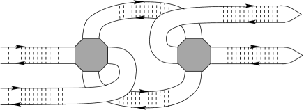
Figure 2: The diagram contributing to the transmission coefficient correlations at large angles. The gray boxes are Hikami boxes, while solid lines connected by dashed lines represent averaged Green functions, see appendix A for details

At this point it is instructive to mention the relation between Eq. (65) and the universal conductance fluctuations of mesoscopic metals. The conductance in these systems is proportional to the integral of the transmission coefficient over the angle, $G\propto\int T(\mbox{\boldmath$\theta$})d\mbox{\boldmath$\theta$}$. Therefore according to Eq. (65) the main contribution to the conductance fluctuations,

$$\langle(\delta G)^{2}\rangle\propto\int d\mbox{\boldmath$\theta$}d\mbox{\boldmath$\theta^{\prime}$}\delta\langle T(\mbox{\boldmath$\theta$})\delta T(\mbox{\boldmath$\theta$}^{\prime})\rangle,$$ (66)

comes from the interval of large angle difference, $\frac{\lambda}{l}<|\mbox{\boldmath$\theta$}-\mbox{\boldmath$\theta^{\prime}$}|$. As a result we have $(\delta G)^{2}\rangle\sim e^{4}/\hbar^{2}$ for a three dimensional system where all dimensions are of the same orderAltshuler ; LeeStone .

IV Conclusions

We have developed a method of description of speckle statistics in elastically scattering media which can be applied to both diffusive and to the ballistic regime. Our main result is given by Eqs. (4-6), which have a form of kinetic equations with random sources. Though the derivation of these equations in Appendix A involved the Born approximation for the amplitude of scattering on individual scatterers, we believe that the region of the applicability of these equation is much broader: They are valid as long as the Boltzmann kinetic equation Eq. (4) holds. Namely, $\ell\gg\lambda,\xi$, and $|{\bf r-r^{\prime}}|\gg\lambda,\xi$.

We would like to mention that the results presented above substantially differ from those known in the literature (see for example Refs. Tatarski, ; Kravtsov, ; Prokhorov, ; Dashen, ). First, the correlation function (40) exhibits a universal long range power law behavior over a wide range of distance, $\rho$. The only non-universal regimes are at the tail, $\rho\gg Z\theta^{2}/\theta_{0}$ , and the short distance region, $\rho\sim\xi$. This result is in contrast with the results presented in Refs. Tatarski, ; Kravtsov, ; Prokhorov, ; Dashen, where the intensity correlator ${\cal C}(\rho)$ depends on the detailed form of the disorder correlation function, $g(r)$, and usually decays exponentially at $\rho>\xi$. Second, ${\cal C}(\rho)$ changes its sign as a function of $\rho$. This property is a consequence of the current conservation and it is absent from previous studies. For instance, the sign change of ${\cal C}(\rho)$ implies, that the fluctuations of the integrated intensity over disks of radius $R>Z\theta$ is proportional to $R$, see Eq. (50), rather than $R^{2}$, as would follow from Refs. Tatarski, ; Kravtsov, ; Prokhorov, ; Dashen, . These differences will affect interpretations of any measurement of speckles done with the help of a sensor aperture that is much larger than the wavelength.

Finally we would like to mention that our results may be easily extended to cases with light polarization, optically active media, Faraday effect, and coherent short wave pulses as long as their duration is longer than $\tau=\ell/c$. These issues are left for future studies.

This work has been supported by the Packard Foundation, by the NSF under Contracts No. DMR-0228104, and by the Israel Science Foundation (ISF) funded by the Israeli Academy of Science and Humanities, and by the USA-Israel Binational Science Foundation (BSF).

Appendix A Derivation of the main equations

The derivation of Eqs. (4), (5), and (6) is based on the standard impurity diagram technique Abrikosov . And the relevant diagram blocks were derived in numerous works. However in most cases the calculations were done either for the case of delta-correlated disorder potential or in the diffusive regime. In this paper we deal with a general situation of an arbitrary angular dependence of the scattering cross-section. Therefore below we outline the derivation of our formalism and present expressions for the main diagram blocks.

The wave equation (1) can be written in the form of a stationary Schrodinger equation for a particle moving in the presence of a random impurity potential,

$$V(\mbox{\boldmath$r$})=-2k^{2}\delta n(\mbox{\boldmath$r$}).$$ (67)

The solution of Eq. (1) can be written as $\psi({\bf r})=\int d{\bf r}^{\prime}G^{R}({\bf r},{\bf r}^{\prime})J({\bf r}^{\prime})$, where $J({\bf r}^{\prime})$ is the source of radiation and $G^{R/A}({\bf r},{\bf r}^{\prime})$ is the retarded Green function, $G^{R/A}\equiv\left(k^{2}+\nabla^{2}-\hat{V}\pm i\eta\right)^{-1}$. Here $\hat{V}$ denotes the impurity potential operator. This reduces the problem of speckle statistics of coherent waves to that of averaging products of retarded and advanced Green functions. The latter problem can be treated using the impurity diagram technique Abrikosov . We derive the expression for the various diagram blocks below.

A.1 Average Green function

In the Born approximation the self-energy, $\Sigma(k,\mbox{\boldmath$p$})$, is given by a single diagram in Fig. 3.

Figure 3: The self-energy diagram in the Born approximation.

Its evaluation gives for the disorder-averaged Green function,

$$G^{R/A}(k,\mbox{\boldmath$p$}) = \frac{1}{k^{2}-p^{2}\pm ik\ell^{-1}},$$ (68)

where the mean free path is given by Eqs. (7) and (8).

A.2 Derivation of the Boltzmann equation

To derive the Boltzmann equation we will need to evaluate products of Green functions at two different frequencies corresponding to wave numbers, $k_{\pm}=k\pm\delta k/2$.

The spatial evolution of the ray distribution function, Eq. (3), can be obtained by expressing the solution of the wave equation in terms of the Green’s functions and performing disorder averaging. In the leading approximation in $\lambda/\ell$ the ray distribution function evolution is described by the sum of ladder diagrams.

Each disorder-averaged Green function is strongly peaked in the momentum region where the on-shell condition is satisfied, $k=|{\bf p}|$. In the limit of dilute scatterers the width of this peak, $\sim 1/\ell$, is much smaller than the typical momentum momentum transfer at each collision. Therefore the integration over the magnitude of momenta in the Green functions can be carried out separately and before the direction integration. Defining $\mathbf{s}$ as the unit vector along the momentum $\mathbf{p}=p\mathbf{s}$ we evaluate the product of the disorder-averaged retarded and advanced Green’s functions integrated over $p$,

$$\frac{1}{\mathcal{B}_{\delta k,\mbox{\boldmath$q$}}(\mbox{\boldmath$s$})} \equiv 4\pi\int_{0}^{\infty}\frac{p^{2}dp}{2\pi^{2}}\,G^{R}(k_{+},p\mbox{\boldmath$s$}+\mbox{\boldmath$q$}/2)G^{A}(k_{-},p\mbox{\boldmath$s$}-\mbox{\boldmath$q$}/2)=\frac{1}{-i\delta k+i\mbox{\boldmath$s$}\mbox{\boldmath$q$}+\ell^{-1}}.$$ (69)

The ray distribution function $f(\mathbf{s},\mathbf{q})$ is given by the sum of ladder diagrams and can be expressed in a compact way using the operator notations,

$$f=\sum_{n=0}^{\infty}\left(\hat{\cal B}^{-1}\hat{W}\right)^{n}f_{0}=\left(\hat{\cal B}-\hat{W}\right)^{-1}\hat{\cal B}f_{0}.$$ (70)

Here $f_{0}$ is the initial ray distribution function, $\hat{\cal B}$ is the integral operator whose kernel in the Fourier representation is given by Eq. (69), and $\hat{W}$ is the integral operator acting in the space of directions,

$$\hat{W}f(\mbox{\boldmath$s$})\equiv\int d\mbox{\boldmath$s$}^{\prime}W(\mbox{\boldmath$s$}-\mbox{\boldmath$s$}^{\prime})f(\mbox{\boldmath$s$}^{\prime}),\quad W(\mbox{\boldmath$s$}-\mbox{\boldmath$s$}^{\prime})\equiv\frac{1}{4\pi}w(k[\mbox{\boldmath$s$}-\mbox{\boldmath$s$}^{\prime}]).$$ (71)

Multiplying Eq. (70) by $\left(\hat{\cal B}-\hat{W}\right)$ from the left and using Eq. (7) we obtain the Boltzmann-Langevin equation,

$$\left(-i\delta k+\mbox{\boldmath$s$}\cdot\nabla_{r}\right)f(\mbox{\boldmath$s$},\mbox{\boldmath$r$})-I_{st}[f]=\mathcal{L},$$ (72)

$$\mathcal{L}=\left(-i\delta k+\mbox{\boldmath$s$}\cdot\nabla_{{\bf r}}+\ell^{-1}\right)f^{0}(\mbox{\boldmath$s$},\mbox{\boldmath$r$}),$$ (73)

where the collision integral $I_{st}[f]$ is defined in Eq. (4).

If one is interested in the average ray distribution function then $f_{0}$ in Eq. (72) should be understood as the ray distribution function of the incident radiation at the boundary of the disordered medium. In this case the source vanishes in the interior of the medium and the average ray distribution function satisfies the usual homogeneous Boltzmann equation.

A.3 Hikami box

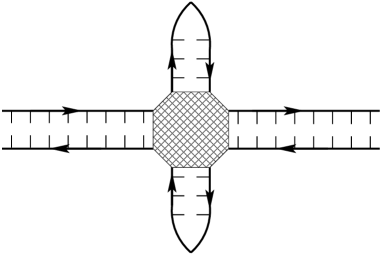
Figure 4: The diagram for the irreducible correlator of ray distribution functions at different points. Two impurity ladders emanating at the radiation source enter the Hikami box, represented by the hashed octagon, from left and right. The ladders going to the observation points leave the Hikami box from the top and the bottom.

Next let us consider the diagram in Fig. 4 that represents the irreducible correlator of the ray distribution functions. It allows the following interpretation which is at the heart of the Boltzmann-Langevin approach developed in this paper. The impurity ladders connecting the observation points to the Hikami box propagate the fluctuations of the distribution function from the Hikami box out to the observation points. This propagation is described by the inhomogeneous Boltzmann-Langevin equation (72). Then the right hand side of Eq. (72) may be interpreted as the “Langevin force” that results in the fluctuations of the ray distribution function. The fluctuations of the Langevin force are described by the Hikami box connected to the impurity ladders going out to the radiation sources. Since the latter define the average ray distribution function we see that by evaluating the Hikami box we will relate the fluctuations of the Langevin force to the average ray distribution function.

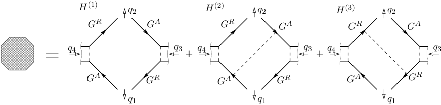
Figure 5: The three diagrams for the Hikami box; $H^{(1)}$, $H^{(2)}$, and $H^{(3)}$. The ladders coming from the radiation sources enter the Hikami box from left and right and are characterized by the four-momenta $q_{3/4}=(\omega_{3/4},\bm{q}_{3/4})$ and the ray directions $\bm{s}_{3/4}$. The ladders going to the observation points exit the Hikami box from the top and the bottom and are characterized by the four-momenta $q_{1/2}=(\omega_{1/2},\bm{q}_{1/2})$ and the ray directions $\bm{s}_{1/2}$. Note that in our notations the Hikami box contains a single impurity line for each of the incoming ladders and no impurity lines for the outgoing ladders.

The Hikami box with the external legs is given by the three diagrams in Fig. 5. It is characterized by the four-momenta $q_{i}=(\omega_{i},\mbox{\boldmath$q$}_{i})$ and the unit vectors $\mbox{\boldmath$s$}_{i}$ characterizing the ray directions. Here $i=1,2$ correspond to outgoing momenta (ladders going to the observation points) and $i=3,4$ to the incoming ones (ladders coming from the radiation source). The momenta satisfy the conservation law, $q_{1}+q_{2}=q_{3}+q_{4}$. The analytic expression that corresponds to the first diagram (with no impurity line) is

$$H^{(1)}_{k}(\{q_{i}\},\{\mbox{\boldmath$s$}_{i}\}) = \delta(\mbox{\boldmath$s$}_{1}-\mbox{\boldmath$s$}_{2})(4\pi)^{2}W(\mbox{\boldmath$s$}_{1}-\mbox{\boldmath$s$}_{3})W(\mbox{\boldmath$s$}_{2}-\mbox{\boldmath$s$}_{4})\int\frac{p^{2}dp}{2\pi^{2}}G^{R}(k+\omega_{1},\mbox{\boldmath$p$}+\mbox{\boldmath$q$}_{1})G^{A}(k,\mbox{\boldmath$p$})$$ (74)

$$\times G^{R}(k+\omega_{4},\mbox{\boldmath$p$}+\mbox{\boldmath$q$}_{4})G^{A}(k+\omega_{1}-\omega_{3},\mbox{\boldmath$p$}+\mbox{\boldmath$q$}_{1}-\mbox{\boldmath$q$}_{3})$$

$$= \frac{\pi}{k^{2}}\delta(\mbox{\boldmath$s$}_{1}-\mbox{\boldmath$s$}_{2})\frac{W(\mbox{\boldmath$s$}_{1}-\mbox{\boldmath$s$}_{3})W(\mbox{\boldmath$s$}_{2}-\mbox{\boldmath$s$}_{4})}{\mathcal{B}_{1}\mathcal{B}_{2}}\left(\frac{1}{\mathcal{B}_{3}}+\frac{1}{\mathcal{B}_{4}}\right),$$

where we used the shorthand notation $\mathcal{B}_{i}=\mathcal{B}_{\delta k_{i},\mbox{\boldmath$q$}_{i}}(\mbox{\boldmath$s$})$ (with $\mbox{\boldmath$s$}=\mbox{\boldmath$s$}_{1}=\mbox{\boldmath$s$}_{2}$) and utilized the momentum conservation, $\mathcal{B}_{1}+\mathcal{B}_{2}=\mathcal{B}_{3}+\mathcal{B}_{4}$.

The second diagram in Fig. 5 contains an impurity line connecting the two advanced Green functions (between $q_{3}$ and $q_{2}$, and $q_{4}$ and $q_{1}$ respectively). It is given by the expression,

$$H^{(2)}_{k}(\{q_{i}\},\{\mbox{\boldmath$s$}_{i}\}) = (4\pi)^{3}W(\mbox{\boldmath$s$}_{1}-\mbox{\boldmath$s$}_{3})W(\mbox{\boldmath$s$}_{2}-\mbox{\boldmath$s$}_{4})W(\mbox{\boldmath$s$}_{1}-\mbox{\boldmath$s$}_{2})\int\frac{p^{2}dp}{2\pi^{2}}G^{R}(k+\omega_{1},\mbox{\boldmath$p$}+\mbox{\boldmath$q$}_{1})G^{A}(k,\mbox{\boldmath$p$})$$ (75)

$$\times G^{A}(k+\omega_{1}-\omega_{3},\mbox{\boldmath$p$}+\mbox{\boldmath$q$}_{1}-\mbox{\boldmath$q$}_{3})\int\frac{p^{\prime 2}dp^{\prime}}{2\pi^{2}}G^{A}(k,\mbox{\boldmath$p$}^{\prime})G^{R}(k+\omega_{4},\mbox{\boldmath$p$}^{\prime}+\mbox{\boldmath$q$}_{4})$$

$$\times G^{A}(k+\omega_{1}-\omega_{3},\mbox{\boldmath$p$}^{\prime}+\mbox{\boldmath$q$}_{1}-\mbox{\boldmath$q$}_{3})$$

$$= -\frac{\pi}{k^{2}}\frac{W(\mbox{\boldmath$s$}_{1}-\mbox{\boldmath$s$}_{3})W(\mbox{\boldmath$s$}_{2}-\mbox{\boldmath$s$}_{4})W(\mbox{\boldmath$s$}_{1}-\mbox{\boldmath$s$}_{2})}{\mathcal{B}_{1}\mathcal{B}^{\prime}_{2}\mathcal{B}_{3}\mathcal{B}^{\prime}_{4}},$$

where unprimed $\mathcal{B}$’s depend on $\mbox{\boldmath$s$}_{1}$ and primed ones on $\mbox{\boldmath$s$}_{2}$,

$$\mathcal{B}_{i} = \mathcal{B}_{\omega_{i},\mbox{\boldmath$q$}_{i}}(\mbox{\boldmath$s$}_{1}),$$ (76)

$$\mathcal{B}^{\prime}_{i} = \mathcal{B}_{\omega_{i},\mbox{\boldmath$q$}_{i}}(\mbox{\boldmath$s$}_{2}).$$ (77)

The third diagram of the Hikami box contains an impurity line connecting the two retarded Green functions (between $q_{1}$ and $q_{3}$, and $q_{2}$ and $q_{4}$ respectively). It is given by

$$H^{(3)}_{k}(\{q_{i}\},\{\mbox{\boldmath$s$}_{i}\}) = (4\pi)^{3}W(\mbox{\boldmath$s$}_{2}-\mbox{\boldmath$s$}_{3})W(\mbox{\boldmath$s$}_{1}-\mbox{\boldmath$s$}_{4})W(\mbox{\boldmath$s$}_{1}-\mbox{\boldmath$s$}_{2})\int\frac{p^{2}dp}{2\pi^{2}}G^{R}(k+\omega_{1},\mbox{\boldmath$p$}+\mbox{\boldmath$q$}_{1})G^{A}(k,\mbox{\boldmath$p$})$$ (78)

$$\times G^{R}(k+\omega_{4},\mbox{\boldmath$p$}+\mbox{\boldmath$q$}_{4})\int\frac{p^{\prime 2}dp^{\prime}}{2\pi^{2}}G^{R}(k+\omega_{1},\mbox{\boldmath$p$}^{\prime}+\mbox{\boldmath$q$}_{1})G^{R}(k+\omega_{4},\mbox{\boldmath$p$}^{\prime}+\mbox{\boldmath$q$}_{4})$$

$$\times G^{A}(k+\omega_{1}-\omega_{3},\mbox{\boldmath$p$}^{\prime}+\mbox{\boldmath$q$}_{1}-\mbox{\boldmath$q$}_{3})$$

$$= -\frac{\pi}{k^{2}}\frac{W(\mbox{\boldmath$s$}_{2}-\mbox{\boldmath$s$}_{3})W(\mbox{\boldmath$s$}_{1}-\mbox{\boldmath$s$}_{4})W(\mbox{\boldmath$s$}_{1}-\mbox{\boldmath$s$}_{2})}{\mathcal{B}_{1}\mathcal{B}^{\prime}_{2}\mathcal{B}^{\prime}_{3}\mathcal{B}_{4}}.$$

Next we make use of the fact that in Eqs. (74), (75), and (78) the operators with indices $3$ and $4$ act on impurity ladders $3$ and $4$ that go out to the radiation sources. These ladders are equal to the average ray distribution functions, $\langle f_{\mbox{\boldmath$s$}}\rangle$. In the interior of the medium the latter obey the Boltzmann equation (72) with the vanishing right hand side, see discussion below Eq. (73). Therefore we have

$$\mathcal{B}^{-1}\hat{W}\langle f_{\mbox{\boldmath$s$}}\rangle=\langle f_{\mbox{\boldmath$s$}}\rangle.$$ (79)

Using Eq. (79) and combining Eqs. (74), (75), and (78) we obtain the correlator of the Langevin forces that enter the right hand side of Eq. (72). As a result we can describe speckle fluctuations in the framework of the Boltzmann-Langevin scheme, Eqs. (5) and (6).

Appendix B Derivation of formula (40)

In this appendix we derive formula (40) for the intensity correlation function in the directed waves limit. For this purpose we employ the parabolic and the Markov approximations. Namely the scalar wave equation (1) is approximated by a simpler equation, obtained by substituting $\psi\to e^{ikz}\psi({\bf r})$ into (1) and neglecting second order derivatives of the wave function with respect to $z$. The resulting equation takes the form of a Schrodinger equation where the coordinated associated with the propagation direction, $z$, plays the role of fictitious time:

$$i\frac{\partial\psi}{\partial z}=-\frac{1}{2k}\left(\frac{\partial^{2}}{\partial x^{2}}+\frac{\partial^{2}}{\partial y^{2}}\right)\psi+k\delta n({\bf r})\psi,$$ (80)

The analysis of this equation is further simplified when the Markov approximation is employed. The latter corresponds to the situation where the disorder correlation function is anisotropic: It is delta correlated in the propagation direction $z$, and long ranged correlated in the perpendicular directions:

$$\langle\delta n({\bf r})\delta n({\bf r}^{\prime})\rangle=g_{\perp}({\mathbf{\rho}}-{\mathbf{\rho}}^{\prime})\delta(z-z^{\prime}).$$ (81)

Here angular brackets denote disorder averaging, and $g_{\perp}(\mbox{\boldmath$\rho$})$ represents the disorder correlation function in the $\mbox{\boldmath$\rho$}=(x,y)$ space. We shall assume that $\delta n({\bf r})$ is gaussian random function and that $g_{\perp}(\mbox{\boldmath$\rho$})$ is isotropic.

These approximations however, do not imply, necessarily, diffusive motion, and therefore applies also for length scales shorter than the mean free path. Within these approximations the Green function associated with, Eq. (4), henceforth called “diffuson” and denoted by ${\cal D}(\mbox{\boldmath$\rho$},{\bf p};z)$, satisfies an equation of the form:

$$\left(\frac{\partial}{\partial z}+\frac{{\bf p}}{k}\frac{\partial}{\partial\mbox{\boldmath$\rho$}}\right){\cal D}(\mbox{\boldmath$\rho$},{\bf p};z)-k^{2}\int\frac{d^{2}q}{4\pi^{2}}\hat{g}_{\perp}({\bf q})\left({\cal D}(\mbox{\boldmath$\rho$},{\bf p}-{\bf q};z)-{\cal D}(\mbox{\boldmath$\rho$},{\bf p};z)\right)=\delta(\mbox{\boldmath$\rho$}-\mbox{\boldmath$\rho$}_{0})\delta({\bf p}-{\bf p}_{0})\delta(z),$$ (82)

where $\hat{g}_{\perp}({\bf q})$ is the Fourier transform of $g_{\perp}(\rho)$. Notice that here the momentum ${\bf p}$ is a two component vector in the space perpendicular to the propagation direction.

The above equation can be simplified by Fourier transforming it with respect to the momentum, ${\bf p}$. Thus if denote by ${\bf x}$ the variable conjugate to the momentum ${\bf p}$, and $\hat{\cal D}$ denotes the Fourier transform of the diffuson ${\cal D}$, then

$$\left(\frac{\partial}{\partial z}-\frac{i}{k}\frac{\partial^{2}}{\partial\mbox{\boldmath$\rho$}\partial{\bf x}}\right)\hat{\cal D}-k^{2}\left[g_{\perp}(x)-g_{\perp}(0)\right]\hat{\cal D}=\frac{e^{i{\bf p}_{0}{\bf x}}}{4\pi^{2}}\delta(\mbox{\boldmath$\rho$}-\mbox{\boldmath$\rho$}_{0})\delta(z).$$ (83)

To solve this equation we further take its Fourier transform with respect to $z$ and $\rho$ (with conjugate variables denoted by $q_{z}$, and ${\bf q}$ respectively):

$$\left(iq_{z}+\frac{\mbox{\boldmath$q$}}{k}\frac{\partial}{\partial{\bf x}}\right)\hat{\cal D}-k^{2}\left[g_{\perp}(x)-g_{\perp}(0)\right]\hat{\cal D}=\frac{e^{i{\bf p}_{0}{\bf x}-i\mbox{\boldmath$q$}\mbox{\boldmath$\rho$}_{0}}}{4\pi^{2}}.$$ (84)

Now let us decompose the vector ${\bf x}$ into its components: $x_{\parallel}$ parallel to the vector $q$, and $x_{\perp}$ perpendicular to that vector. Then the solution of the above equation takes the form:

$$\hat{\cal D}=\frac{ke^{-i\mbox{\boldmath$q$}\mbox{\boldmath$\rho$}_{0}}}{4\pi^{2}q}\int_{-\infty}^{x_{\parallel}}dx_{\parallel}^{\prime}e^{ip_{0\parallel}x_{\parallel}^{\prime}+ip_{0\perp}x_{\perp}}\exp\frac{k}{q}\left[\int_{x_{\parallel}^{\prime}}^{x_{\parallel}}dx_{\parallel}^{\prime\prime}\left(iq_{z}-k^{2}\left(g_{\perp}(x_{\parallel}^{\prime\prime},x_{\perp})-g_{\perp}(0)\right)\right)\right],$$ (85)

where under the assumption of isotropy in the plane perpendicular to the propagation direction $g_{\perp}(x_{\parallel},x_{\perp})=g_{\perp}\left(\sqrt{x^{2}_{\parallel}+x_{\perp}^{2}}\right)$. Now, taking the inverse Fourier transform with respect to $q_{z}$, integrating over $x_{\parallel}^{\prime}$, and Fourier transforming the result with respect to ${\bf x}$ we obtain the result for the diffuson:

$${\cal D}(\mbox{\boldmath$\rho$},{\bf p};\mbox{\boldmath$\rho$}_{0},{\bf p}_{0};z)=\int\frac{d^{2}x}{4\pi^{2}}\int\frac{d^{2}q}{4\pi^{2}}e^{i\mbox{\boldmath$q$}(\mbox{\boldmath$\rho$}-\mbox{\boldmath$\rho$}_{0})+i{\bf p}_{0}\left({\bf x}-\frac{z}{k}\mbox{\boldmath$q$}\right)-i{\bf p}{\bf x}}\exp\left[\frac{k^{3}}{q}\int_{x_{\parallel}-\frac{q}{k}z}^{x_{\parallel}}dx_{\parallel}^{\prime\prime}\left(g_{\perp}(x_{\parallel}^{\prime\prime},x_{\perp})-g_{\perp}(0)\right)\right].$$ (86)

If we assume boundary conditions where the average distribution function, at $z=0$, is given by $\bar{f}_{0}(\mbox{\boldmath$\rho$},{\bf p})$, then for $z>0$ the average distribution function is given by the integral:

$$\bar{f}(\mbox{\boldmath$\rho$},{\bf p},z)=\int d^{2}\rho_{0}d^{2}p_{0}{\cal D}(\mbox{\boldmath$\rho$},{\bf p};\mbox{\boldmath$\rho$}_{0},{\bf p}_{0};z)\bar{f}_{0}(\mbox{\boldmath$\rho$}_{0},{\bf p}_{0})$$ (87)

In particular assuming the incident wave, at $z=0$, to be a plane wave pointing at the $z$ direction, $\bar{f}_{0}(\mbox{\boldmath$\rho$},{\bf p})=4\pi^{2}I_{0}\delta({\bf p})$ where $I_{0}$ is the density, the above integral reduces to

$$\bar{f}({\bf p},z)=I_{0}\int d^{2}x\exp\left[-i{\bf p}{\bf x}-2k^{2}\left(g_{\perp}(x)-g_{\perp}(0)\right)\right]$$ (88)

This formula is exact assuming the parabolic and the Markov approximation. Namely it holds as long as $l\gg\xi$ (Markov approximation), and $\xi\gg\lambda$ (small angle scattering, i.e. parabolic approximation). It holds for any distance $z<l_{tr}$, and for any value of the momentum ${\bf p}$. It may be further simplified if we assume $z\gg\ell$ where $\ell$ is the elastic mean free path. In this case the dynamics is of diffusive nature in the angle of directions and one may approximate the correlation function $g_{\perp}(x)$ using Taylor expansion near $x=0$:

$$g_{\perp}(x)\simeq g_{\perp}(0)-D_{\theta}x^{2}$$ (89)

where $D_{\theta}=-g_{\perp}^{\prime\prime}(0)/2$ ($g_{\perp}^{\prime\prime}(x)$ denote the second derivative of $g_{\perp}(x)$ with respect to $x$) is the angular diffusion constant. Substituting (89) into (88) and preforming the integral over $x$ yields:

$$\bar{f}({\bf p},z)\simeq\frac{\pi I_{0}}{k^{2}D_{\theta}z}\exp\left[-\frac{p^{2}}{4k^{2}D_{\theta}z}\right],~{}~{}~{}~{}~{}z\gg l$$ (90)

Let us now consider the fluctuations of the distribution function. Using Eqs. (5) and (6), one may write their corresponding correlation function as

$$\langle\delta f(\mbox{\boldmath$\rho$},{\bf p},Z)\delta f(\mbox{\boldmath$\rho$}^{\prime},{\bf p}^{\prime},Z)\rangle=\int_{0}^{Z}dz\int d^{2}\rho^{\prime\prime}d^{2}p_{1}d^{2}p_{2}{\cal D}(\mbox{\boldmath$\rho$},{\bf p};\mbox{\boldmath$\rho$}^{\prime\prime},{\bf p}_{1};Z-z)~{}~{}~{}~{}~{}~{}~{}~{}~{}~{}~{}~{}~{}~{}~{}~{}~{}~{}~{}~{}~{}~{}~{}~{}~{}~{}~{}~{}~{}~{}~{}~{}~{}~{}$$ (91)

$$\times\left(g_{\perp}(0)\delta({\bf p}_{1}-{\bf p}_{2})-\hat{g}_{\perp}({\bf p}_{1}-{\bf p}_{2})\right)\bar{f}({\bf p}_{1},z)\bar{f}({\bf p}_{2},z){\cal D}(\mbox{\boldmath$\rho$}^{\prime},{\bf p}^{\prime};\mbox{\boldmath$\rho$}^{\prime\prime},{\bf p}_{2};Z-z)$$

where, as before, this result has been obtained under the parabolic and the Markov approximations. The density correlation function, ${\cal C}(\mbox{\boldmath$\rho-\rho^{\prime}$}$ can be deduced from (91) by integration over ${\bf p}$ and ${\bf p}^{\prime}$:

$$C(\mbox{\boldmath$\rho$}-\mbox{\boldmath$\rho$}^{\prime})=\int d^{2}pd^{2}p^{\prime}\langle\delta f(\mbox{\boldmath$\rho$},{\bf p},Z)\delta f(\mbox{\boldmath$\rho$}^{\prime},{\bf p}^{\prime},Z)\rangle$$ (92)

Thus substituting (91) and (86) into the above formula, a and performing the integral over $\mbox{\boldmath$\rho$}^{\prime\prime}$ yields

$$C(\mbox{\boldmath$\rho$})=\int_{0}^{Z}d\zeta\int\frac{d^{2}q}{4\pi^{2}}\frac{d^{2}p_{1}}{4\pi^{2}}\frac{d^{2}p_{2}}{4\pi^{2}}\left(g_{\perp}(0)\delta({\bf p}_{1}-{\bf p}_{2})-\hat{g}_{\perp}({\bf p}_{1}-{\bf p}_{2})\right)\bar{f}({\bf p}_{1},\zeta)\bar{f}({\bf p}_{2},\zeta)~{}~{}~{}~{}~{}~{}$$ (93)

$$\times\exp\left[i\mbox{\boldmath$q$}\left(\mbox{\boldmath$\rho$}-\frac{{\bf p}_{1}-{\bf p_{2}}}{k}(Z-\zeta)\right)+2k^{2}\int_{0}^{Z-\zeta}d\eta\left(g(\eta q/k)-g(0)\right)\right]$$

This formula is obtained essentially by introducing one Hikami box into the diagrams. The small parameter controlling this approximation (i.e. the neglect of additional Hikami boxes) is $l\gg\xi^{2}/\lambda$. The distance between the observation points should be larger than the disorder correlation length, $|\mbox{\boldmath$\rho$}-\mbox{\boldmath$\rho$}^{\prime}|>\xi$.

The above integral can be further simplified if we assume the width of the system, $Z$, to be much larger than the elastic mean free path, $Z\gg l$. In that case, as can be seen from formula (90), the width of the average distribution function $\bar{f}({\bf p},\zeta)$ at $\zeta\gg\ell$ is much wider than the width of $\hat{g}_{\perp}({\bf p})$, as the width of first function is $k\sqrt{D_{\theta}\zeta}\sim\frac{1}{\xi}\sqrt{\zeta/\ell}$, while the second is of order $1/\xi$. Therefore, assuming the integral over $z$ to be dominated by points near the screen $z=Z$ (an assumption which turns out to be consistent) one may approximate the factor $\bar{f}({\bf p}_{1},\zeta)\bar{f}({\bf p}_{2},\zeta)$ in the integral (91) as $\bar{f}({\bf p}_{1},\zeta)\bar{f}({\bf p}_{2},\zeta)\simeq\bar{f}^{2}({\bf p}_{1},\zeta))$, and consider ${\bf p}_{1}$ and $\tilde{\bf p}={\bf p}_{2}-{\bf p}_{1}$ as independent variables. Since in this regime $\bar{f}({\bf p},\zeta)$ is given by Eq. (90) the integral over $p_{1}$ and $p_{2}-p_{1}$ can be performed and the result takes is

$$C(\rho)=\frac{\pi I_{0}^{2}}{D_{\theta}}\int_{\ell}^{Z}\frac{d\zeta}{\zeta}\int\frac{d^{2}q}{4\pi^{2}}\left(g_{\perp}(0)-g_{\perp}\left(\frac{q(Z-\zeta)}{k}\right)\right)\exp\left[i\mbox{\boldmath$q$}\mbox{\boldmath$\rho$}+2k^{2}\int_{0}^{Z-\zeta}d\eta\left(g(\eta q/k)-g(0)\right)\right].$$ (94)

Performing the angular part of the integral over $q$, expressing the pre-exponential factor as a derivative of the exponent, and changing the integration variable from $\zeta$ to $Z-\zeta$ we finally obtain formula (40):

$$C(\rho)=\frac{I_{0}^{2}}{4D_{\theta}k^{2}}\int_{0}^{Z-\ell}\frac{d\zeta}{\zeta-Z}\int qdqJ_{0}(q\rho)\frac{d}{d\zeta}\exp\left[-\frac{2}{\ell}\int_{0}^{\zeta}d\eta\left(1-\tilde{g}\left(\frac{q}{k}\eta\right)\right)\right],$$ (95)

where $\ell^{-1}=k^{2}g_{\perp}(0)$, while $\tilde{g}(\eta)=g_{\perp}(\eta)/g_{\perp}(0)$.

References

• (1) J.W. Goodman, in Laser Speckles and Related Phenomena, edited by J.C. Dainty, (Spinger-Verlag Berlin, 1975).
• (2) B.Z. Spivak, A.Yu. Zyuzin, Sov. Phys. JETP 66, 560, (1987).
• (3) S. Feng, C.L. Kane, P.A. Lee, A.D. Stone, Phys. Rev. B 61, 834, (1988).
• (4) A.Ju. Zyuzin, B.Z. Spivak, in Mesoscopic Phenomena in Solids vol. 30, ed. by B. Altshuler, P.A. Lee, R.Webb (Noth-Holland, Elsevier Science Publisher,(1991).
• (5) S.M. Rytov, Yu.A. Kravtsov, V.I. Tatarskii, Principles of statistical radiophysics, Vol 4 Springer-Verlag, (1989).
• (6) Yu.A. Kravtsov, Rep. Prog. Phys. 39, (1992).
• (7) A.M. Prokhorov, F.V. Bunkin, K.S. Gochelashvily, V.I. Shishov, Proc. IEEE, 63, 790, (1975).
• (8) R. Dashen, J. Math. Phys. 20, 894, (1979).
• (9) L. D. Landau and E. M. Lifshitz, Statistical Physics, Part I, Addison-Wesley (1969).
• (10) Sh. M. Kogan and A. Ya. Shul’man, Zh. Eksp. Teor. Fiz. 56, 862 (1969) [Sov. Phys. JETP 29, 467 (1969)].
• (11) Sh. Kogan, Electronic noise and fluctuations in solids, Cambridge University Press (1996).
• (12) S. V. Gantsevich, V.L. Gurevich, and R. Katilius. Zh. Eksp. Teor. Fiz. 57 no. 2, 503 (1969) [Sov. Phys.- JETP 30 no. 2, 276 (1970)]; Revista del Nuovo Cimento 2 No. 5, 1 (1979).
• (13) O. Agam, A. V. Andreev, and B. Spivak, Phys. Rev. Lett. 97, 223901 (2006).
• (14) A.A. Abrikosov, L.P. Gorkov, I.E. Dzialoshinskii, Methods of Quantum Field Theory in Statistical Physics, Dover, (1968).
• (15) B.L. Altshuler, B.Z. Spivak, JETP Lett. 42, 447 (1985).
• (16) B.L. Altshuler, JETP Lett. 41, 648, (1985).
• (17) Spivak, A. Zyuzin, Sol. State Comm. 65, 311 (1988.)
• (18) The procedure of averaging in the classical case, and the concept of the fluctuations of the distribution function $\delta\tilde{f}$ require some clarification. The classical kinetic equation Eq. (11) is valid in systems which exhibit chaotic partiocle dynamics, which means that the kinetics of the system has a self-averaging character. Thus the averaging procedure denoted by the double brackets $\langle\langle\ldots\rangle\rangle$ does not include averaging over the random configurations of the scattering potential. The classical kinetic scheme does not necesserily require an introduction of the fluctuations of the distribution function $\delta\tilde{f}$. There is another approach to claculation of classical nonequilibrium fluctuations GurevichGanzevichKatilus , which is equvalent to Eqs. (11), (12), and (13), and is based on equations for the sigle $\langle\langle\tilde{f}\rangle\rangle$ and two particle $\langle\langle\delta\tilde{f}\delta\tilde{f}\rangle\rangle$ distribution functions.
• (19) A. M. Jayannavar and N. Kumar, Phys. Rev. Lett. 48, 553 (1982).
• (20) P.A. Lee, A.D. Stone, Phys. Rev. Lett. 55, 1622, (1985).