Reliability of Coupled Oscillators I:
Two-Oscillator Systems

Abstract

This paper concerns the reliability of a pair of coupled oscillators in response to fluctuating inputs. Reliability means that an input elicits essentially identical responses upon repeated presentations regardless of the network’s initial condition. Our main result is that both reliable and unreliable behaviors occur in this network for broad ranges of coupling strengths, even though individual oscillators are always reliable when uncoupled. A new finding is that at low input amplitudes, the system is highly susceptible to unreliable responses when the feedforward and feedback couplings are roughly comparable. A geometric explanation based on shear-induced chaos at the onset of phase-locking is proposed.

Introduction

This paper, together with its companion paper Reliability of Coupled Oscillators II, contain a mathematical treatment of the question of reliability. Reliability here refers to whether a system produces identical responses when it is repeatedly presented with the same stimulus. Such questions are relevant to signal processing in biological and engineered systems. Consider, for example, a network of inter-connected neurons with some background activity. An external stimulus in the form of a time-dependent signal is applied to this neural circuitry, which processes the signal and produces a response in the form of voltage spikes. We say the system is reliable if, independent of its state at the time of presentation, the same stimulus elicits essentially identical responses following an initial period of adjustment. That is, the response to a given signal is reproducible [32, 5, 27, 28, 47, 39, 34, 30, 22, 13, 14, 38].

This study is carried out in the context of (heterogeneous) networks of interconnected oscillators. We assume the input signal is received by some components of the network and relayed to others, possibly in the presence of feedback connections. Our motivation is a desire to understand the connection between a network’s reliability properties and its architecture, i.e. its “circuit diagram,” the strengths of various connections, etc. This problem is quite different from the simpler and much studied situation of uncoupled oscillators driven by a common input. In the latter, the concept of reliability coincides with synchronization, while in coupled systems, internal synchronization among constituent components is not a condition for reliability.

To simplify the analysis, we assume the constituent oscillators are phase oscillators or circle rotators, and that they are driven by a fluctuating input which, for simplicity, we take to be white noise. Under these conditions, systems consisting of a single, isolated phase oscillator have been explored extensively and shown to be reliable; see, e.g.,  [39, 34]. Our results are presented in a two-part series:

Paper I.  Two-oscillator systems

Paper II.  Larger networks

The present paper contains an in-depth analysis of a 2-oscillator system in which the stimulus is received by one of the oscillators. Our results show that such a system can support both reliable and unreliable dynamics depending on coupling constants; a more detailed discussion of the main points of this paper is given later in the Introduction. Paper II extends some of the ideas developed in this paper to larger networks that can be decomposed into subsystems or “modules” so that the inter-module connections form an acyclic graph. At the level of inter-module connections, such “acyclic quotient networks” have essentially feedforward dynamics; they are reliable if all the component modules are also reliable. Acyclic quotient networks are allowed to contain unreliable modules, however, and the simplest example of such a module is, as shown in this paper, an oscillator pair with nontrivial feedforward-feedback connections. In Paper II, we also explore issues surrounding the creation and propagation of unreliability in larger networks.

With regard to aims and methodology, we seek to identify and explain relevant phenomena, and to make contact with rigorous mathematics whenever we can, hoping in the long run to help bring dynamical systems theory closer to biologically relevant systems. The notion of reliability, for example, is prevalent in neuroscience. With all the idealizations and simplifications at this stage of our modeling, we do not expect our results to be directly applicable to real-life situations, but hope that on the phenomenological level they will shed light on systems that share some characteristics with the oscillator networks studied here. Rigorous mathematical results are presented in the form of “Theorems,” “Propositions,” etc., and simulations are used abundantly. Our main results are qualitative. They are a combination of rigorous statements and heuristic explanations supported by numerical simulations and/or theoretical understanding.

Content of present paper

A motivation for this work is the following naive (and partly rhetorical) question: Are networks of coupled phase oscillators reliable, and if not, how large must a network be to exhibit unreliable behavior? Our answer to this question is that unreliable behavior occurs already in the 2-oscillator configuration in Diagram (1). Our results demonstrate clearly that such a system can be reliable or unreliable, and that both types of behaviors are quite prominent, depending in a generally predictable way on the nature of the feedforward and feedback connections. Furthermore, we identify geometric mechanisms responsible for these behaviors.

Referring the reader again to Diagram (1), three of the system’s parameters are $a_{\rm ff}$ and $a_{\rm fb}$, the feedforward and feedback coupling constants, and $\varepsilon$, the amplitude of the stimulus. The following is a preview of the main points of this paper:

1. Lyapunov exponents as a measure of reliability. Viewing the stimulus-driven system as described by a stochastic differential equation and leveraging existing results from random dynamical systems theory, we explain in Sect. 2 why the top Lyapunov exponent ($\lambda_{\rm max}$) of the associated stochastic flow is a reasonable measure of reliability. In this interpretation, reliability is equated with $\lambda_{\rm max}<0$, which is known to be equivalent to having random sinks in the dynamics, while unreliability is equated with $\lambda_{\rm max}>0$, which is equivalent to the presence of random strange attractors.

2. Geometry and zero-input dynamics. In pure feedforward and feedback configurations, i.e., at $a_{\rm fb}=0$ or $a_{\rm ff}=0$, we identify geometric structures that prohibit unreliability. Our main result about zero-input systems is on phase-locking: in Sect. 3.3, we prove that for all $a_{\rm ff}$ in a broad range, the system is 1:1 phase-locked for either $a_{\rm fb}\gtrsim a_{\rm ff}$ or $a_{\rm fb}\lesssim a_{\rm ff}$ depending on the relative intrinsic frequencies of the two oscillators. This phenomenon has important consequences for reliability.

3. Shear-induced chaos as main cause for unreliability at low drive amplitudes. Recent advances in dynamical systems theory have identified a mechanism for producing chaos via the interaction of a forcing with the underlying shear in a system. The dynamical environment near the onset of phase-locking is particularly susceptible to this mechanism. We verify in Sect. 4.2 that the required “shearing” is indeed present in our 2-oscillator system. Applying the cited theory, we are able to predict the reliability or lack thereof for coupling parameters near the onset of phase-locking. At low drive amplitudes, this is the primary cause for unreliability.

4. Reliability profile as a function of $a_{\rm ff},a_{\rm fb}$ and $\varepsilon$. Via numerical simulations and theoretical reasoning, we deduce a rough reliability profile for the 2-oscillator system as a function of the three parameters above. With the increase in $|a_{\rm ff}|,|a_{\rm fb}|$ and/or $\varepsilon$, both reliable and unreliable regions grow in size and become more robust, meaning $\lambda_{\rm max}$ is farther away from zero. The main findings are summarized in Sect. 4.3.

1 Model and Formulation

1.1 Description of the model

We consider in this paper a small network consisting of two coupled phase oscillators forced by an external stimulus as shown:

(1)

We assume the coupling is via smooth pulsatile interactions as in [37, 45, 8, 12], and the equations defining the system are given by

$$\begin{array}[]{rcl}\dot{\theta}_{1}&=&\omega_{1}+a_{\rm fb}\ z(\theta_{1})\ g(\theta_{2})+\varepsilon z(\theta_{1})\ I(t)\ ,\\ \dot{\theta}_{2}&=&\omega_{2}+a_{\rm ff}\ z(\theta_{2})\ g(\theta_{1})\ .\\ \end{array}$$ (2)

The state of each oscillator is described by a phase, i.e., an angular variable $\theta_{i}\in{\mathbb{S}}^{1}\equiv{\mathbb{R}}/{\mathbb{Z}},i=1,2$. The constants $\omega_{1}$ and $\omega_{2}$ are the cells’ intrinsic frequencies. We allow these frequencies to vary, but assume for definiteness that they are all within about $10\%$ of $1$. The external stimulus is denoted by $\varepsilon I(t)$. Here $I(t)$ is taken to be white noise, and $\varepsilon$ is the signal’s amplitude. Notice that the signal is received only by cell 1. The coupling is via a “bump function” $g$ which vanishes outside of a small interval $(-b,b)$. On $(-b,b)$, $g$ is smooth, it is $\geq 0$, has a single peak, and satisfies $\int_{-b}^{b}{g(\theta)\ d\theta}=1$. The meaning of $g$ is as follows: We say the $i$th oscillator “spikes” when $\theta_{i}(t)=0$. Around the time that an oscillator spikes, it emits a pulse which modifies the other oscillator. The sign and magnitude of the feedforward coupling is given by $a_{\rm ff}$ (“forward” refers to the direction of stimulus propagation): $a_{\rm ff}>0$ (resp. $a_{\rm ff}<0$) means oscillator 1 excites (resp. inhibits) oscillator 2 when it spikes. The feedback coupling, $a_{\rm fb}$, plays the complementary role. In this paper, $b$ is taken to be about $\frac{1}{20}$, and $a_{\rm ff}$ and $a_{\rm fb}$ are taken to be ${\mathcal{O}}(1)$. Finally, $z(\theta)$, often called the phase response curve [44, 15, 8, 4, 23], measures the variable sensitivity of an oscillator to coupling and stimulus input. In this paper, we take $z(\theta)=\frac{1}{2\pi}(1-\cos(2\pi\theta))$ (see below).

1.2 Neuroscience interpretations

Coupled phase oscillators arise in many settings [32, 35, 23, 19, 45, 33]. Here, we briefly discuss their use in mathematical neuroscience.

We think of phase oscillators as paradigms for systems with rhythmic behavior. Such models are often derived as limiting cases of oscillator models in two or more dimensions. In particular, the specific form of $z(\cdot)$ chosen here corresponds to the normal form for oscillators near saddle-node bifurcations on their limit cycles [8]. This situation is typical in neuroscience, where neural models with $z(\theta)\approx 1-\cos(\cdot)$ are referred to as “Type I.” The pulse- or spike-based coupling implemented by $g(\cdot)$ may also be motivated by the synaptic impulses sent between neurons after they fire action potentials (although this is not the only setting in which pulsatile coupling arises [45, 3, 10, 37, 36, 18, 29, 31, 19]).

The general conclusions that we will present do not depend on the specific choices of $z(\cdot)$ and $g(\cdot)$, but rather on their qualitative features. Specifically, we have checked that our main results about reliability and phase locking are essentially unchanged when the $z(\cdot)$ function becomes asymmetric and the location of the $g(\cdot)$ impulse is somewhat shifted, as would correspond more closely to neuroscience [8]. Therefore, the behavior we find here can be expected to be fairly prototypical for pairs of pulse-coupled Type I oscillators.

A standard way to investigate the reliability of a system of spiking oscillators — both in the laboratory and in simulations — is to repeat the experiment using a different initial condition each time but driving the system with the same stimulus $\varepsilon I(t)$, and to record spike times in raster plots. Fig. 1 shows such a raster plot for an isolated oscillator of the present type, as studied by [34, 16]. Note that, for each repetition, the oscillator produces essentially identical spike times after a transient, demonstrating its reliability.

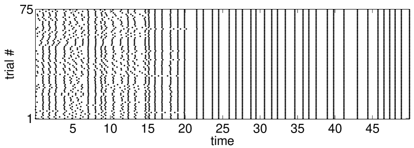
Figure 1: Raster plot for an isolated oscillator. In each experiment, 75 trials are performed, and dots are placed at spike times. Nearly identical spike times are observed after a transient, indicating reliability.

2 Measuring Reliability

All of the ideas discussed in this section are general and are easily adapted to larger networks.

2.1 A working definition of reliability

We attempt to give a formal definition of reliability in a general setting. Consider a dynamical system on a domain $M$ (such as a manifold or a subset of Euclidean space). A signal in the form of $\iota(t)\in{\mathbb{R}}^{n},t\in[0,\infty),$ is presented to the system. The response $F(t)$ of the system to this signal is given by $F(t)=F(x_{0},t,\{\iota(s)\}_{0\leq s<t})$. That is to say, the response at time $t$ may, in principle, depend on $x_{0}\in M$, the initial state of the system when the signal is presented, and the values of the signal up to time $t$.

In the model as described in Sect. 1.1, $F(t)$ can be thought of as the pair $(\theta_{1}(t),\theta_{2}(t))$ or $\Psi(\theta_{1}(t),\theta_{2}(t))$, the value of an observable at time $t$.

We propose now one way to define reliability. Given a dynamical system, a class of signals $\cal I$, and a response function $F$, we say the system is reliable if for almost all $\iota\in{\cal I}$ and $x_{0},x_{0}^{\prime}\in M$,

$$\|F(x_{0},t,\{\iota(s)\}_{0\leq s<t})-F(x_{0}^{\prime},t,\{\iota(s)\}_{0\leq s<t})\|\to 0\quad{\rm as}\quad t\to\infty\ .$$

Here $\|\cdot\|$ is a norm on the range space of $F$. We do not claim that this is the only way to capture the idea of reliability, but will use it as our operational definition.

We point out some of the pitfalls of this definition: In practice, signals are never presented for infinite times, and in some situations, responses can be regarded as reliable only if the convergence above is rapid. By the same token, not all initial conditions are equally likely, leaving room for probabilistic interpretations.

Finally, one should not expect unreliable responses to be fully random. On the contrary, as we will show in Sect. 2.2, they tend to possess a great deal of structure, forming what are known as random strange attractors.

2.2 Reliability, Lyapunov exponents, and random attractors

We discuss here some mathematical tools that can be used to quantify how reliable or unreliable a driven system is. With $I(t)$ taken to be realizations of white noise, (2) can be put into the framework of a random dynamical system (RDS). We begin by reviewing some relevant mathematics [1, 2]. Consider a general stochastic differential equation

$$dx_{t}=a(x_{t})\ dt+\sum_{i=1}^{k}b_{i}(x_{t})\circ dW^{i}_{t}\ .$$ (3)

In this general setting, $x_{t}\in M$ where $M$ is a compact Riemannian manifold, the $W^{i}_{t}$ are independent standard Brownian motions, and the equation is of Stratonovich type. Clearly, Eq. (2) is a special case of Eq. (3): $x_{t}$ describes the phases of the $2$ oscillators, $M={\mathbb{T}}^{2}\equiv{\mathbb{S}}^{1}\times{\mathbb{S}}^{1}$ (thus we have the choice between the Itô or Stratonovich integral), and $k=1$.

In general, one fixes an initial $x_{0}$, and looks at the distribution of $x_{t}$ for $t>0$. Under fairly general conditions, these distributions converge to a unique stationary measure $\mu$, the density of which is given by the Fokker-Planck equation. Since reliability is about a system’s reaction to a single stimulus, i.e., a single realization of the $W^{i}_{t}$, at a time, and concerns the simultaneous evolution of all or large ensembles of initial conditions, of relevance to us are not the distributions of $x_{t}$ but flow-maps of the form $F_{t_{1},t_{2};\omega}$. Here $t_{1}<t_{2}$ are two points in time, $\omega$ is a sample Brownian path, and $F_{t_{1},t_{2};\omega}(x_{t_{1}})=x_{t_{2}}$ where $x_{t}$ is the solution of (3) corresponding to $\omega$. A well known theorem states that such stochastic flows of diffeomorphisms are well defined if the functions $a(x)$ and $b(x)$ in Eq. (3) are sufficiently smooth. More precisely, the maps $F_{t_{1},t_{2};\omega}$ are well defined for almost every $\omega$, and they are invertible, smooth transformations with smooth inverses. Moreover, $F_{t_{1},t_{2};\omega}$ and $F_{t_{3},t_{4};\omega}$ are independent for $t_{1}<t_{2}<t_{3}<t_{4}$. These results allow us to treat the evolution of systems described by (3) as compositions of random, i.i.d., smooth maps. Many of the techniques for analyzing smooth deterministic systems have been extended to this random setting. We will refer to the resulting body of work as RDS theory.

Similarly, the stationary measure $\mu$, which gives the steady-state distribution averaged over all realizations $\omega$, does not describe what we see when studying a system’s reliability. Of relevance are the sample measures $\{\mu_{\omega}\}$, which are the conditional measures of $\mu$ given the past. Here we think of $\omega$ as defined for all $t\in(-\infty,\infty)$ and not just for $t>0$. Then $\mu_{\omega}$ describes what one sees at $t=0$ given that the system has experienced the input defined by $\omega$ for all $t<0$. This is an idealization: in reality, the input is presented on a time interval $[-t_{0},0)$ for some $t_{0}>0$. Two useful facts about these sample measures are

• $(F_{-t,0;\omega})_{*}\mu\to\mu_{\omega}$ as $t\to\infty$, where $(F_{-t,0;\omega})_{*}\mu$ is the measure obtained by transporting $\mu$ forward by $F_{-t,0;\omega}$, and

• the family $\{\mu_{\omega}\}$ is invariant in the sense that $(F_{0,t;\omega})_{*}(\mu_{\omega})=\mu_{\sigma_{t}(\omega)}$ where $\sigma_{t}(\omega)$ is the time-shift of the sample path $\omega$ by $t$.

Thus, if our initial distribution is given by a probability density $\rho$ and we apply the stimulus corresponding to $\omega$, then the distribution at time $t$ is $(F_{0,t;\omega})_{*}\rho$. For $t$ sufficiently large, one expects in most situations that $(F_{0,t;\omega})_{*}\rho$ is very close to $(F_{0,t;\omega})_{*}\mu$, which by (a) above is essentially given by $\mu_{\sigma_{t}(\omega)}$. The time-shift by $t$ of $\omega$ is necessary because by definition, $\mu_{\omega}$ is the conditional distribution of $\mu$ at time $0$.

Fig. 2 shows some snapshots of $(F_{0,t;\omega})_{*}\rho$ for the coupled oscillator pair in the system (1) for two different sets of parameters. In the panels corresponding to $t\gg 1$, the distributions approximate $\mu_{\sigma_{t}(\omega)}$. In these simulations, the initial distribution $\rho$ is the stationary density of Eq. (2) with $\varepsilon\approx 0.01$, the interpretation being that the system is intrinsically noisy even in the absence of external stimuli. Observe that these pictures evolve with time, and as $t$ increases they acquire similar qualitative properties depending on the underlying system. This is in agreement with RDS theory, which tells us in fact that the $\mu_{\sigma_{t}(\omega)}$ obey a statistical law for almost all $\omega$. Observe also the strikingly different behaviors in the top and bottom panels. We will follow up on this observation presently. First, we recall two mathematical results that describe the dichotomy.

$t=20$	$t=50$	$t=500$	$t=1900$

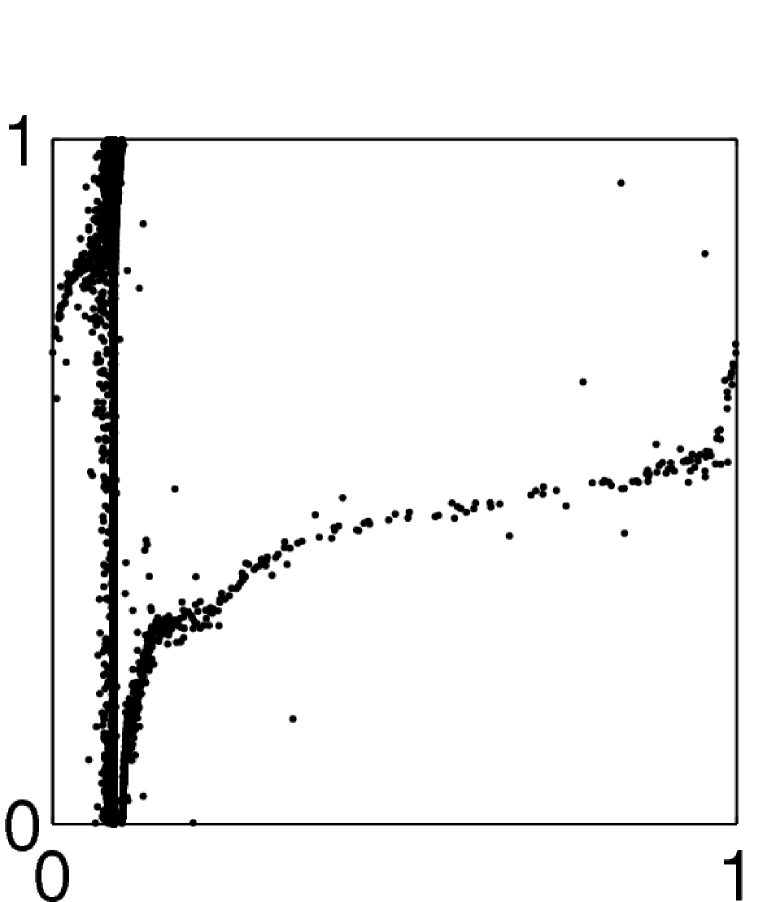
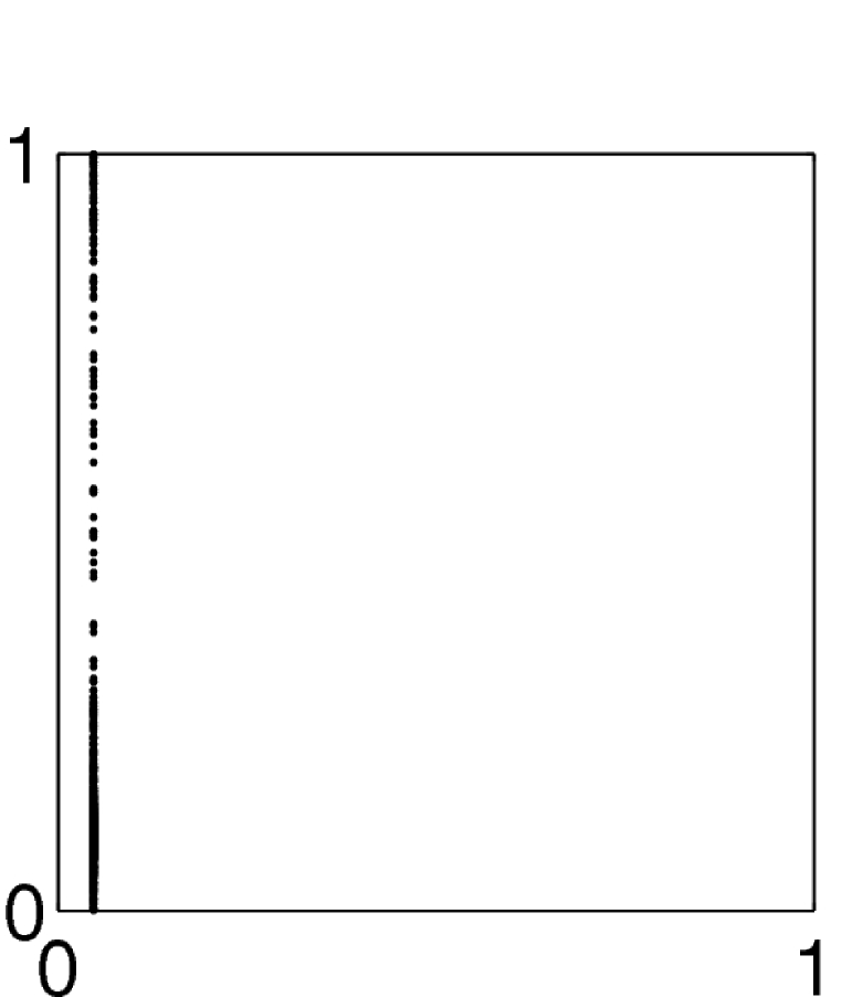
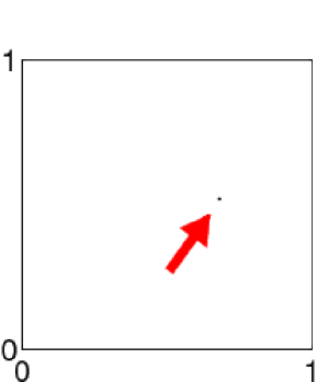
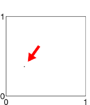
(a) Random fixed point ($\lambda_{\rm max}<0$)

$t=20$	$t=50$	$t=500$	$t=1900$

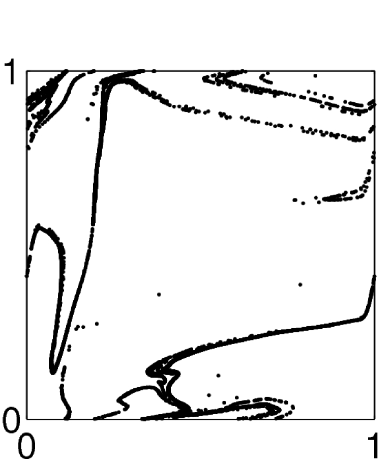
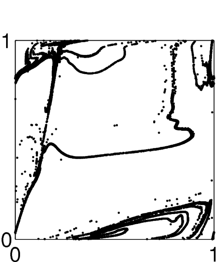
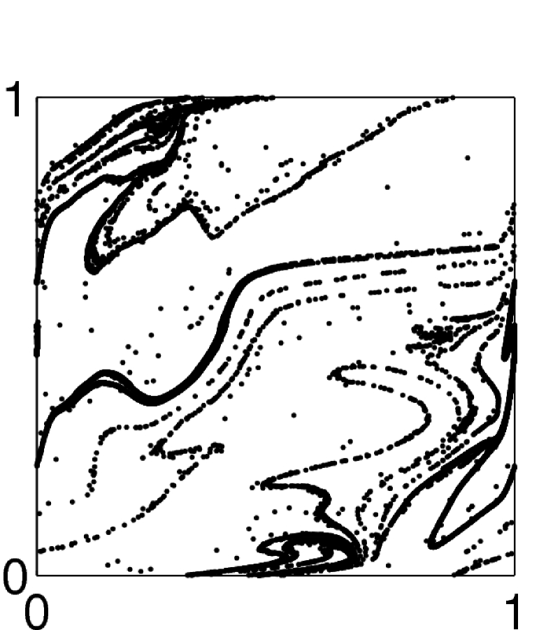
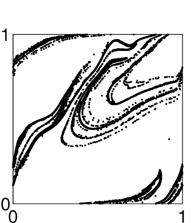
(b) Random strange attractor ($\lambda_{\rm max}>0$)

Figure 2: Snapshots of sample measures for Eq. (2) at various times in response to a single realization of the stimulus. Two different sets of parameters are used in (a) and (b). In (a), the sample measures converge to a random fixed point. In (b), the sample measures converge to a random strange attractor. See Theorem 1.

In deterministic dynamics, Lyapunov exponents measure the exponential rates of separation of nearby trajectories. Let $\lambda_{\max}(x)$ denote the largest Lyapunov exponent along the trajectory starting from $x$. Then a positive $\lambda_{\max}$ for a large set of initial conditions is generally thought of as synonymous with chaos, while the presence of stable equilibria is characterized by $\lambda_{\max}<0$. For smooth random dynamical systems, Lyapunov exponents are also known to be well defined; moreover, they are nonrandom, i.e. they do not depend on $\omega$. If, in addition, the invariant measure is erogdic, then $\lambda_{\max}$ is constant almost everywhere in the phase space. In Theorem 1 below, we present two results from RDS theory that together suggest that the sign of $\lambda_{\rm max}$ is a good criterion for distinguishing between reliable and unreliable behavior:

Theorem 1.

In the setting of Eq. (3), let $\mu$ be an ergodic stationary measure.

• (Random sinks) [20] If $\lambda_{\max}<0$, then with probability 1, $\mu_{\omega}$ is supported on a finite set of points.

• (Random strange attractors) [24] If $\mu$ has a density and $\lambda_{\max}>0$, then with probability 1, $\mu_{\omega}$ is a random SRB measure.

The conclusion of Part (1) is interpreted as follows: The scenario in which the support of $\mu_{\omega}$ consists of a single point corresponds exactly to reliability for almost every $\omega$ as defined in Sect. 2.1. This was noted in, e.g., [34, 30]. For the $2$-oscillator system defined by Eq. (2), the collapse of all initial conditions to a point is illustrated in Fig. 2(a); notice that $\mu_{\sigma_{t}\omega}$ continues to evolve as $t$ increases. Even though in general $\mu_{\omega}$ can be supported on more than one point when $\lambda_{\rm max}<0$, this seems seldom to be the case except in the presence of symmetries. We do not know of a mathematical result to support this empirical observation, however. In the rest of this paper, we will take the liberty to equate $\lambda_{\rm max}<0$ with reliability.

The conclusion of Part (2) requires clarification: In deterministic dynamical systems theory, SRB measures are natural invariant measures that describe the asymptotic dynamics of chaotic dissipative systems (in the same way that Liouville measures are the natural invariant measures for Hamiltonian systems). SRB measures are typically singular. They are concentrated on unstable manifolds, which are families of curves, surfaces etc. that wind around in a complicated way in the phase space [7]. Part (2) of Theorem 1 generalizes these ideas to random dynamical systems. Here, random (meaning $\omega$-dependent) SRB measures live on random unstable manifolds, which are complicated families of curves, surfaces, etc. that evolve with time. In particular, in a system with random SRB measures, different initial conditions lead to very different outcomes at time $t$ when acted on by the same stimulus; this is true for all $t>0$, however large. It is, therefore, natural to regard $\lambda_{\max}>0$ and the distinctive geometry of random SRB measures as a signature of unreliability.

In the special case where the phase space is a circle, such as in the case of a single oscillator, that the Lyapunov exponent $\lambda$ is $\leq 0$ is an immediate consequence of Jensen’s Inequality. In more detail,

$$\lambda(x)\ =\lim_{t\rightarrow\infty}\frac{1}{t}\log F^{\prime}_{0,t;\omega}(x)$$

for typical $\omega$ by definition. Integrating over initial conditions $x$, we obtain

$$\lambda\ =\int_{{\mathbb{S}}^{1}}\lim_{t\rightarrow\infty}\frac{1}{t}\log F^{\prime}_{0,t;\omega}(x)\ dx=\lim_{t\rightarrow\infty}\frac{1}{t}\int_{{\mathbb{S}}^{1}}\log F^{\prime}_{0,t;\omega}(x)\ dx\ .$$

The exchange of integral and limit is permissible because the required integrability conditions are satisfied in stochastic flows [21]. Jensen’s Inequality then gives

$$\int_{{\mathbb{S}}^{1}}\log F^{\prime}_{0,t;\omega}(x)\ dx\ \leq\ \log\int_{{\mathbb{S}}^{1}}F^{\prime}_{0,t;\omega}(x)\ dx\ =\ 0\ .$$ (4)

The equality above follows from the fact that $F_{0,t;\omega}$ is a circle diffeomorphism. Since the gap in the inequality in (4) is larger when $F^{\prime}_{0,t;\omega}$ is farther from being a constant function, we see that $\lambda<0$ corresponds to $F^{\prime}_{0,t;\omega}$ becoming “exponentially uneven” as $t\to\infty$. This is consistent with the formation of random sinks.

The following results from general RDS theory shed light on the situation when the system is multi-dimensional:

Proposition 2.1.

(see e.g. [21]) In the setting of Eq. (3), assume $\mu$ has a density, and let $\{\lambda_{1},\cdots,\lambda_{d}\}$ be the Lyapunov exponents of the system counted with multiplicity. Then

(i) $\sum_{i}\lambda_{i}\leq 0$;

(ii) $\sum_{i}\lambda_{i}=0$ if and only if $F_{s,t,\omega}$ preserves $\mu$ for almost all $\omega$ and all $s<t$;

(iii) if $\sum_{i}\lambda_{i}<0$, and $\lambda_{i}\neq 0$ for all $i$, then $\mu_{\omega}$ is singular.

A formula giving the dimension of $\mu_{\omega}$ is proved in [24] under mild additional conditions.

The reliability of a single oscillator, i.e. that $\lambda<0$, is easily deduced from Prop. 2.1: $\mu$ has a density because the transition probabilities have densities, and no measure is preserved by all the $F_{s,t,\omega}$ because different stimuli distort the phase space differently. Prop. 2.1(i) and (ii) together imply that $\lambda<0$. See also, e.g., [30, 28, 39, 34].

The remarks above concerning $\mu$ apply also to the $2$-oscillator model in Eq. (2). (That $\mu$ has a density is explained in more detail in Sect. 3.2.) Therefore, Prop. 2.1(i) and (ii) together imply that $\lambda_{1}+\lambda_{2}<0$. Here $\lambda_{1}=\lambda_{\rm max}$ can be positive, zero, or negative. If it is $>0$, then it will follow from Prop. 2.1(i) that $\lambda_{2}<0$, and by Prop. 2.1(iii), the $\mu_{\omega}$ are singular. From the geometry of random SRB measures, we conclude that different initial conditions are attracted to lower dimensional sets that depend on stimulus history. Thus even in unreliable dynamics, the responses are highly structured and far from uniformly distributed, as illustrated in Fig. 2(b).

Finally, we observe that since $\lambda_{\rm max}$ is nonrandom, the reliability of a system is independent of the realization $\omega$ once the stimulus amplitude $\varepsilon$ is fixed.

3 Coupling geometry and zero-input dynamics

3.1 Preliminary observations

First we describe the flow $\varphi_{t}$ on the 2-torus $\mathbb{T}^{2}$ defined by Eq. (2) when the stimulus is absent, i.e., when $\varepsilon=0$. We begin with the case where the two oscillators are uncoupled, i.e. $a_{\rm ff}=a_{\rm fb}=0$. In this special case, $\varphi_{t}$ is a linear flow; depending on whether $\omega_{1}/\omega_{2}$ is rational, it is either periodic or quasiperiodic. Adding coupling distorts flow lines inside the two strips $\{|\theta_{1}|<b\}$ and $\{|\theta_{2}|<b\}$. These two strips correspond to the regions where one of the oscillators “spikes,” transmitting a coupling impulse to the other (see Sect. 1.1). For example, if $a_{\rm ff}>0$, then an orbit entering the vertical strip containing $\theta_{1}=0$ will bend upward. Because of the variable sensitivity of the receiving oscillator, the amount of bending depends on $a_{\rm ff}$ as well as the value of $\theta_{2}$, with the effect being maximal near $\theta_{2}=\frac{1}{2}$ and negligible near $\theta_{2}=0$ due to our choice of the function $z(\theta)$. The flow remains linear outside of these two strips. See Fig. 3.

Because the phase space is a torus and Eq. (2) does not have fixed points for the parameters of interest, $\varphi_{t}$ has a global section, e.g., $\Sigma_{0}=\{\theta_{2}=0\}$, with a return map $T_{0}:\Sigma_{0}\to\Sigma_{0}$. The large-time dynamics of $\varphi_{t}$ are therefore described by iterating $T_{0}$, a circle diffeomorphism. From standard theory, we know that circle maps have Lyapunov exponents $\leq 0$ for almost all initial conditions with respect to Lebesgue measure. This in turn translates into $\lambda_{\rm max}=0$ for the flow $\varphi_{t}$.

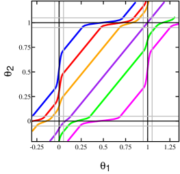
(a) $a_{\rm ff}=1,a_{\rm fb}=1.5$

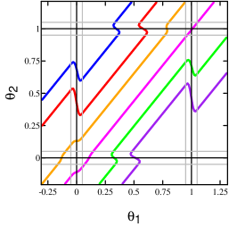
(b) $a_{\rm ff}=-1,a_{\rm fb}=-0.5$

Figure 3: Plots of a few orbits of Eq. (2) with $\varepsilon=0$ showing the strips in which flowlines are distorted. In both sets, $\omega_{1}=1,\omega_{2}=1.1$. Note the directions of bending in relation to the signs of $a_{\rm ff}$ and $a_{\rm fb}$.

3.2 Reliability of two special configurations

We consider next two special but instructive cases of Eq. (2), namely the “pure feedforward” case corresponding to $a_{\rm fb}=0$ and the “pure feedback” case corresponding to $a_{\rm ff}=0$. We will show that in these two special cases, the geometry of the system prohibits it from being unreliable:

Proposition 3.1.

For every $\varepsilon>0$,

• the system (2) has an ergodic stationary measure $\mu$ with a density;

• (i) if $a_{\rm fb}=0$, then $\lambda_{\rm max}\leq 0$;

  (ii) if $a_{\rm ff}=0$, then $\lambda_{\rm max}=0$.

We first discuss these results informally. Consider the case $a_{\rm fb}=0$. Notice that when $\varepsilon=0$, the time-$t$ map of the flow generated by Eq. (2) sends vertical circles (meaning sets of the form $\{\theta_{1}=c\}$ where $c$ is a constant) to vertical circles. As our stimulus acts purely in the horizontal direction and its magnitude is independent of $\theta_{2}$, vertical circles continue to be preserved by the flow-maps $F_{s,t,\omega}$ when $\varepsilon>0$. (One can also see this from the variational equations.) As is well known, $\lambda_{\rm max}>0$ usually results from repeated stretching and folding of the phase space. Maps that preserve all vertical circles are far too rigid to allow this to happen. Thus we expect $\lambda_{\rm max}\leq 0$ when $a_{\rm fb}=0$. In the pure feedback case $a_{\rm ff}=0$, the second oscillator rotates freely without input from either external stimuli or the first oscillator. Thus the system always has a zero Lyapunov exponent corresponding to the uniform motion in the direction of $\theta_{2}$.

Before proving Proposition 3.1, we recall some properties of Lyapunov exponents. Let $F_{0,t;\omega}$ denote the stochastic flow on ${\mathbb{T}}^{2}$, and let $\mu$ be a stationary measure of the process. Recall that for a.e. $\omega$, $\mu$-a.e. $x\in{\mathbb{T}}^{2}$ and every tangent vector $v$ at $x$, the Lyapunov exponent

$$\lambda_{\omega}(x,v)\ =\ \lim_{t\to\infty}\ \frac{1}{t}\log|DF_{0,t;\omega}(x)v|$$

is well defined. Moreover, if $\lambda_{1}\leq\lambda_{2}$ are the Lyapunov exponents at $x$, then

$$\lim_{t\to\infty}\ \frac{1}{t}\log|\det(DF_{0,t;\omega}(x))|\ =\ \lambda_{1}+\lambda_{2}\ .$$ (5)

We say $\{v_{1},v_{2}\}$ is a Lyapunov basis at $x$ if $\lambda_{\omega}(x,v_{i})=\lambda_{i}$. It follows from (5) that for such a pair of vectors,

$$\lim_{t\to\infty}\ \frac{1}{t}\log|\sin\angle(DF_{0,t;\omega}(x)v_{1},DF_{0,t;\omega}(x)v_{2})|=0,$$ (6)

that is, angles between images of vectors in a Lyapunov basis do not decrease exponentially fast. It is a standard fact that Lyapunov bases exist almost everywhere, and that any nonzero tangent vector can be part of such a basis.

Proof of Proposition 3.1.

First, we verify that Eq. (2) has a stationary measure with a density. Because the white noise stimulus $\varepsilon I(t)$ instantaneously spreads trajectories in the horizontal ($\theta_{1}$) direction, an invariant measure must have a density in this direction. At the same time, the deterministic part of the flow carries this density forward through all of ${\mathbb{T}}^{2}$ since flowlines make approximately 45 degree angles with the horizontal axis. Therefore the two-oscillator system has a 2-D invariant density whenever $\varepsilon>0$.

We discuss the pure feedforward case. The case of $a_{\rm ff}=0$ is similar and is left to the reader.

As noted above, when $a_{\rm fb}=0$ the flow $F_{0,t;\omega}$ leaves invariant the family of vertical circles. This means that $F_{0,t;\omega}$ factors onto a stochastic flow on the first circle. More precisely, if $\pi:{\mathbb{T}}^{2}={\mathbb{S}}^{1}\times{\mathbb{S}}^{1}\to{\mathbb{S}}^{1}$ is projection onto the first factor, then for almost every $\omega$ and every $s<t$, there is a diffeomorphism $\bar{F}_{0,t;\omega}$ of ${\mathbb{S}}^{1}$ with the property that for all $x\in{\mathbb{T}}^{2}$, $\pi(F_{0,t;\omega}(x))=\bar{F}_{0,t;\omega}(\pi(x))$. One checks easily that $\bar{F}_{s,t;\omega}$ is in fact the stochastic flow corresponding to the system in which oscillator 2 is absent and oscillator 1 alone is driven by the stimulus. For simplicity of notation, for $x\in{\mathbb{T}}^{2}$ and tangent vector $v$ at $x$, we denote $\pi(x)$ by $\bar{x}$ and $D\pi(x)\cdot v$ by $\bar{v}$. Furthermore, we let $\bar{\lambda}_{\omega}$ denote the Lyapunov exponent of $\bar{F}_{s,t;\omega}$. From Prop. 2.1, it follows that $\bar{\lambda}_{\omega}<0$ almost everywhere.

We now consider the Lyapunov exponents of system (2). At $\mu$-a.e. $x\in{\mathbb{T}}^{2}$, we pick a vector $v$ in the $\theta_{2}$-direction. Since $F_{0,t;\omega}$ preserves vertical circles and $\mu$ has a density, an argument similar to that before Prop. 2.1 gives $\lambda_{\omega}(x,v)\leq 0$. Let $\{u,v\}$ be a Lyapunov basis at $x$. From Eq. (6) and the relation between $F_{0,t;\omega}$, and $\bar{F}_{s,t;\omega}$, we deduce that

$$\lambda_{\omega}(x,u)=\lim_{t\to\infty}\ \frac{1}{t}\log|\overline{DF_{0,t;\omega}(x)\cdot u}|=\lim_{t\to\infty}\ \frac{1}{t}\log|{D\bar{F}_{0,t;\omega}(\bar{x})\cdot\bar{u}}|=\bar{\lambda}_{\omega}(\bar{x},\bar{u})<0\ .$$

∎

It is likely that $\lambda_{\rm max}$ is typically $<0$ in the case $a_{\rm fb}=0$. We have shown that one of the Lyapunov exponents, namely the one corresponding to the first oscillator alone, is $<0$. The value of $\lambda_{\rm max}$ therefore hinges on $\lambda_{\omega}(x,v)$ for vectors $v$ without a component in the $\theta_{1}$-direction. Even though this growth rate also involves compositions of random circle maps, the maps here are not i.i.d.: the kicks received by the second oscillator are in randomly timed pulses that cannot be put into the form of the white noise term in Eq. (3). We know of no mathematical result that guarantees a strictly negative Lyapunov exponent in this setting, but believe it is unlikely that Eq. (3) will have a robust zero Lyapunov exponent unless $a_{\rm ff}=0$.

To summarize, we have shown that without recurrent connections, it is impossible for a two-oscillator system to exhibit an unreliable response.

3.3 Phase locking in zero-input dynamics

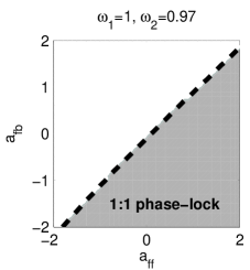
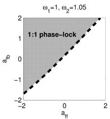
Figure 4: The critical value $a_{\rm fb}^{*}$ as functions of $a_{\rm ff}$. In both plots, the dashed line is the $a_{\rm fb}^{*}$ curve (see text), and the shaded regions are the parameters for which 1:1 phase-locking occurs.

This subsection is about the dynamics of the coupled oscillator system when $\varepsilon=0$. Recall that the intrinsic frequencies of the two oscillators, $\omega_{1}$ and $\omega_{2}$, are assumed to be $\approx 1$. Our main result is that if $\omega_{1}$ and $\omega_{2}$ differ by a little, then in regions of the $(a_{\rm ff},a_{\rm fb})$-parameter plane in the form of a square centered at $(0,0)$, the two oscillators are 1:1 phase-locked for about half of the parameters. Two examples are shown in Fig. 4, and more detail will be given as we provide a mathematical explanation for this phenomenon. (Phase locking of pairs of coupled phase oscillators is studied in e.g., [12, 17, 8, 9, 6, 37]. A primary difference is that we treat the problem on an open region of the $(a_{\rm ff},a_{\rm fb})$-plane centered at $(0,0)$.)

Let $\varphi_{t}$ be the flow on ${\mathbb{T}}^{2}$ defined by (2) with $\varepsilon=0$. To study $\varphi_{t}$, we consider its return map $T:\Sigma_{b}\to\Sigma_{b}$ where $\Sigma_{b}=\{\theta_{2}=b\}$. Working with the section $\Sigma_{b}$ (as opposed to e.g. $\Sigma_{0}$) simplifies the analysis as we will see, and substantively the results are not section dependent. Let $\rho(T)$ be the rotation number of $T$. Since $\omega_{1}\approx\omega_{2}$, it is natural to define $\rho(T)$ in such a way that $\rho(T)\approx 1$ when $a_{\rm ff}=a_{\rm fb}=0$, so that $\rho(T)$ may be interpreted as the average number of rotations made by the first oscillator for each rotation made by the second. It is well known that if $\rho(T)$ is irrational, then $\varphi_{t}$ is equivalent to a quasi-periodic flow via a continuous change of coordinates, while $\rho(T)\in{\mathbb{Q}}$ corresponds to the presence of periodic orbits for $\varphi_{t}$. In particular, attracting fixed points of $T$ correspond to attracting periodic orbits of $\varphi_{t}$ that are 1:1 phase-locked, “1:1” here referring to the fact that oscillator 2 goes around exactly once for each rotation made by oscillator 1.

We begin with the following elementary facts:

Lemma 3.1.

• With $\omega_{1}$, $\omega_{2}$, and $a_{\rm ff}$ fixed and letting $T=T_{a_{\rm fb}}$, the function $a_{\rm fb}\mapsto T_{a_{\rm fb}}(\theta_{1})$ is strictly increasing for each $\theta_{1}$; it follows that $\rho(T_{a_{\rm fb}})$ is a nondecreasing function of $a_{\rm fb}$.

• With $\omega_{1}$, $a_{\rm ff}$, and $a_{\rm fb}$ fixed, $\omega_{2}\mapsto T_{\omega_{2}}(\theta_{1})$ is strictly decreasing for each $\theta_{1}$, and $\rho(T_{\omega_{2}})$ is a non-increasing function of $\omega_{2}$.

Analogous results hold as we vary $a_{\rm ff}$ and $\omega_{1}$ separately keeping the other three quantities fixed.

Proof.

This follows from the way each coupling term bends trajectories; see Sect. 3.1 and Fig. 3. We show (a); the rest are proved similarly. Consider two trajectories, both starting from the same point on $\Sigma_{b}$ but with different $a_{\rm fb}$. They will remain identical until their $\theta_{2}$-coordinates reach $1-b$, as $a_{\rm fb}$ does not affect this part of the flow. Now at each point in the horizontal strip $H=\{1-b<\theta_{2}<1+b\}$, the vector field corresponding to the larger $a_{\rm fb}$ has a larger horizontal component while the vertical components of the two vector fields are identical. It follows that the trajectory with the larger $a_{\rm fb}$ will be bent farther to the right as it crosses $H$. ∎

Our main result identifies regions in parameter space where $T$ has a fixed point, corresponding to 1:1 phase-locking as discussed above. We begin with the following remarks and notation: (i) Observe that when $\omega_{1}=\omega_{2}$ and $a_{\rm ff}=a_{\rm fb}$, we have ${T}(x)=x$ for all $x\in\Sigma_{b}$; this is a consequence of the symmetry of $z(\theta)$ about $\theta=\frac{1}{2}$. (ii) We introduce the notation $\Delta\omega=1-\frac{\omega_{1}}{\omega_{2}}$, so that when $a_{\rm ff}=a_{\rm fb}=0$, $x-T(x)=\Delta\omega$ for all $x$, i.e., $\Delta\omega$ measures the distance moved by the return map $T$ under the linear flow when the two oscillators are uncoupled. Here, we have used $T$ to denote not only the section map but its lift to $\mathbb{R}$ with $T(1)=1$ in a harmless abuse of notation.

We will state our results for a bounded range of parameters. For definiteness, we consider $a_{\rm ff},a_{\rm fb}\in[-2,2]$ and $.9\leq\omega_{i}\leq 1.1$. The bounds for $a_{\rm ff}$ and $a_{\rm fb}$ are quite arbitrary. Once chosen, however, they will be fixed; in particular, the constants in our lemmas below will depend on these bounds. It is implicitly assumed that all parameters considered in Theorem 2 are in this admissible range. We do not view $b$ as a parameter in the same way as $\omega_{1},\omega_{2},a_{\rm ff}$ or $a_{\rm fb}$, but instead of fixing it at $\frac{1}{20}$, we will take $b$ as small as need be, and assume $|g|={\mathcal{O}}(\frac{1}{b})$ in the rigorous results to follow.

Theorem 2.

The following hold for all admissible $(\omega_{1},\omega_{2},a_{\rm ff},a_{\rm fb})$ and all $b$ sufficiently small:

• If $\omega_{2}>\omega_{1}$, then there exist $a_{\rm fb}^{*}=a_{\rm fb}^{*}(\omega_{1},\omega_{2},a_{\rm ff})>a_{\rm ff}$ and $\ell=\ell(\Delta\omega)>0$ such that $T$ has a fixed point for $a_{\rm fb}\in[a_{\rm fb}^{*},a_{\rm fb}^{*}+\ell]$ and no fixed point for $a_{\rm fb}<a_{\rm fb}^{*}$.

• If $\omega_{2}<\omega_{1}$, then there exist $a_{\rm fb}^{*}=a_{\rm fb}^{*}(\omega_{1},\omega_{2},a_{\rm ff})<a_{\rm ff}$ and $\ell=\ell(\Delta\omega)>0$ such that $T$ has a fixed point for $a_{\rm fb}\in[a_{\rm fb}^{*}-\ell,a_{\rm fb}^{*}]$ and no fixed point for $a_{\rm fb}>a_{\rm fb}^{*}$.

Moreover, $|a_{\rm fb}^{*}-a_{\rm ff}|={\mathcal{O}}(\Delta\omega)$; and for each $\Delta\omega\neq 0$, $\ell$ increases as $b$ decreases.

To prove this result, we need two lemmas, the proofs of both of which are given in the Appendix. Define $\Delta a_{\rm fb}=a_{\rm fb}-a_{\rm ff}$.

Lemma 3.2.

There exist $b_{1}$ and $K>0$ such that for all admissible $(\omega_{1},\omega_{2},a_{\rm ff},a_{\rm fb})$, if $b<b_{1}$ and $\Delta a_{\rm fb}<Kb^{-2}\Delta\omega$, then $T(1-b)<1-b$.

Lemma 3.3.

There exist $b_{2},C>0$ and $x_{1}\in(0,1-b)$ such that for all admissible $(\omega_{1},\omega_{2},a_{\rm ff},a_{\rm fb})$, if $b<b_{2}$ and $\Delta a_{\rm fb}>C\Delta\omega$, then $T(x_{1})>x_{1}$.

Proof of Theorem 2..

We prove (a); the proof of (b) is analogous. Let $\omega_{1},\omega_{2}$ and $a_{\rm ff}$ be given. Requirements on the size of $b$ will emerge in the course of the proof.

Observe first that with $\omega_{2}>\omega_{1}$, $T$ has no fixed point (and hence there is no 1:1 phase locking) when $a_{\rm fb}=a_{\rm ff}$. This is because $T(x)=x$ when $\omega_{2}=\omega_{1}$ and $a_{\rm fb}=a_{\rm ff}$ as noted earlier, and using Lemma 3.1(b), we see that for $\omega_{2}>\omega_{1}$ and $a_{\rm fb}=a_{\rm ff}$, the graph of ${T}$ is strictly below the diagonal.

Keeping $\omega_{1},\omega_{2}$ and $a_{\rm ff}$ fixed, we now increase $a_{\rm fb}$ starting from $a_{\rm fb}=a_{\rm ff}$. By Lemma 3.1(a), this causes the graph of ${T}$ to shift up pointwise. As $a_{\rm fb}$ is gradually increased, we let $a_{\rm fb}^{*}$ be the first parameter at which the graph of ${T}$ intersects the diagonal, i.e. where there exists $x^{*}\in\Sigma_{b}$ such that ${T}(x^{*})=x^{*}$ — if such a parameter exists. Appealing once more to Lemma 3.1, we see that $\rho(T)<1$ for all $a_{\rm fb}<a_{\rm fb}^{*}$, so $T$ can have no fixed point for these values of $a_{\rm fb}$.

We show now that $a_{\rm fb}^{*}$ exists, and that the phase-locking persists on an interval of $a_{\rm fb}$ beyond $a_{\rm fb}^{*}$. First, if $b$ is small enough, then by Lemma 3.2, $T(1-b)<1-b$ for all $a_{\rm fb}<a_{\rm ff}+Kb^{-2}\Delta\omega$. Now if $b$ is small enough that $Kb^{-2}>C$ where $C$ is as in Lemma 3.3, then for $a_{\rm fb}\in[a_{\rm ff}+C\Delta\omega,a_{\rm ff}+Kb^{-2}\Delta\omega]$, $T(x_{1})>x_{1}$ for some $x_{1}<1-b$. For $a_{\rm fb}$ in this range, $T$ maps the interval $[x_{1},1-b]$ into itself, guaranteeing a fixed point. It follows that (i) $a_{\rm fb}^{*}$ exists and is $<a_{\rm ff}+C\Delta\omega$, and (ii) $T$ has a fixed point for an interval of $a_{\rm fb}$ of length $\ell\geq(Kb^{-2}-C)\Delta\omega$. This completes the proof. ∎

As noted in the proof, for as long as $\omega_{2}\neq\omega_{1}$, the lengths of the phase-locked intervals, $\ell$, can be made arbitrarily large by taking $b$ small. On the other hand, if we fix $b$ and shrink $\Delta\omega$, then these intervals will shrink. This is consistent with the phenomenon that the phase-locked region lies on opposite sides of the diagonal $a_{\rm fb}=a_{\rm ff}$ when we decrease $\omega_{2}$ past $\omega_{1}$, as shown in Fig. 4.

Instead of tracking the numerical constants in the proofs, we have checked numerically that for $b=\frac{1}{20}$, the pictures in Fig. 4 are quite typical, meaning about $50\%$ of the parameters are phase locked. Specifically, for $\Delta\omega$ up to about $10\%$ and $|a_{\rm ff}|<2$, $a_{\rm fb}^{*}-a_{\rm ff}\lesssim 0.2$, so that the $a_{\rm fb}^{*}$-curve describing the onset of phase-locking is still quite close to the diagonal $a_{\rm ff}=a_{\rm fb}$. Also, for $\Delta\omega$ as small as $\frac{1}{2}\%$, the phase locked intervals have length $\ell>4$. These facts together imply that for parameters in the admissible range, the pictures are as shown in Fig. 4.

Figure 5: The rotation number $\rho$ and Lyapunov exponent $\lambda_{\rm min}$ as functions of $a_{\rm fb}$.

Fig. 5 shows numerically-computed rotation numbers $\rho$ and the rates of contraction to the corresponding limit cycle, i.e. the smaller Lyapunov exponent $\lambda_{\rm min}$ of the flow $\varphi_{t}$. Notice that as $a_{\rm fb}$ increases past $a_{\rm fb}^{*}$, $\lambda_{\rm min}$ decreases rapidly, so that the fixed point of $T$ becomes very stable, a fact consistent with the large interval on which the system is 1:1 phase-locked. Furthermore, for the full range of $|a_{\rm ff}|,|a_{\rm fb}|\leq 2$ and $0.9\leq\omega_{i}\leq 1.1$, we find numerically that $0.53<\rho(T)<1.89$. Phase-locking corresponding to rational $\rho(T)$ with small denominators $q$ (e.g., $q=3,4,5$) is detected, but the intervals are very short and their lengths decrease rapidly with $q$. In other words, when the system is not 1:1 phase-locked – which occurs for about $50\%$ of the parameters of interest – modulo fine details the system appears to be roughly quasi-periodic over not too large timescales. When the white-noise stimulus $\varepsilon I(t)$ is added, these fine details will matter little.

4 Reliable and Unreliable Behavior

Numerical evidence is presented in Sect. 4.2 showing that unreliability can occur even when the stimulus amplitude is relatively small, and that its occurrence is closely connected with the onset of phase-locking in the zero-input system. A geometric explanation in terms of shear-induced chaos is proposed. Additionally, other results leading to a qualitative understanding of $\lambda_{\rm max}$ as a function of $a_{\rm ff},a_{\rm fb}$ and $\varepsilon$ are discussed in Sect. 4.3.

4.1 A brief review of shear-induced chaos

A rough idea of what we mean by “shear-induced chaos” is depicted in Fig. 6: An external force is transiently applied to a limit cycle (horizontal line), causing some phase points to move up and some to move down. Suppose the speeds with which points go around the limit cycle are height dependent. If the velocity gradient, which we refer to as “shear”, is steep enough, then the bumps created by the forcing are exaggerated as the system relaxes, possibly causing the periodic orbit to fold. Such folding has the potential to lead to the formation of strange attractors. If the damping is large relative to the velocity gradient or the perturbation size, however, the bumps in Fig. 6 will dissipate before any significant stretching occurs.

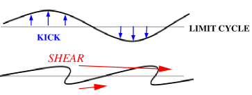
Figure 6: The stretch-and-fold action of a kick followed by relaxation in the presence of shear.

This subsection reviews a number of ideas surrounding the mechanism above. This mechanism is known to occur in many different dynamical settings. We have elected to introduce the ideas in the context of discrete-time kicking of limit cycles instead of the setting of Eq. (2) because the geometry of discrete-time kicks is more transparent, and many of the results have been shown numerically to carry over with relatively minor modifications. Extensions to relevant settings are discussed later on in this subsection. A part of this body of work is supported by rigorous analysis. Specifically, theorems on shear-induced chaos for periodic kicks of limit cycles are proved in [40, 41, 42, 43]; it is from these articles that many of the ideas reviewed here have originated. Numerical studies extending the ideas in [41, 42] to other types of underlying dynamics and forcing are carried out in [26]. For readers who wish to see a more in-depth (but not too technical) account of the material in this subsection, [26] is a good place to start. In particular, Sect. 1 in [26] contains a fairly detailed exposition of the rigorous work in [40, 41, 42, 43].

Discrete-time kicks of limit cycles

We consider a flow $\varphi_{t}$ in any dimension, with a limit cycle $\gamma$. Let $T_{0}<T_{1}<T_{2}<\cdots$ be a sequence of kick times, and let $\kappa_{n},n=0,1,2,\cdots$, be a sequence of kick maps (for the moment $\kappa_{n}$ can be any transformation of the phase space). We consider a system kicked at time $T_{n}$ by $\kappa_{n}$, with ample time to relax between kicks, i.e., $T_{n+1}-T_{n}$ should not be too small on average.

Central to the geometry of shear-induced chaos is the following dynamical structure of the unforced system: For each $x\in\gamma$, the strong stable manifold $W^{ss}(x)$ of $\varphi_{t}$ through $x$ is defined to be

$$W^{ss}(x)=\{y:\lim_{t\to\infty}d(\varphi_{t}(x),\varphi_{t}(y))=0\}\ .$$

These codimension 1 submanifolds are invariant under the flow, meaning $\varphi_{t}$ carries $W^{ss}(x)$ to $W^{ss}(\varphi_{t}(x))$. In particular, if $\tau$ is the period of the limit cycle, then $\varphi_{\tau}(W^{ss}(x))=W^{ss}(x)$ for each $x$. Together these manifolds partition the basin of attraction of $\gamma$ into hypersurfaces, forming what is called the strong stable foliation.

Fig. 7 shows a segment $\gamma_{0}\subset\gamma$, its image $\gamma_{0}^{+}=\kappa(\gamma)$ under a kick map $\kappa$, and two images of $\gamma_{0}^{+}$ under $\varphi_{n\tau}$ and $\varphi_{m\tau}$ for $n>m\in{\mathbb{Z}}^{+}$. If we consider integer multiples of $\tau$, so that the flow-map carries each $W^{ss}$-leaf to itself, we may think of it as sliding points in $\gamma_{0}^{+}$ toward $\gamma$ along $W^{ss}$-leaves. (For $t$ that are not integer multiples of $\tau$, the picture is similar but shifted along $\gamma$.) The stretching created in this combined kick-and-slide action depends both on the geometry of the $W^{ss}$-foliation and on the action of the kick. Fig. 7 sheds light on the types of kicks that are likely to lead to folding: A forcing that drives points in a direction roughly parallel to the $W^{ss}$-leaves will not produce folding. Nor will kicks that essentially carry one $W^{ss}$-leaf to another, because such kicks necessarily preserve the ordering of the leaves. What causes the stretching and folding is the variation along $\gamma$ in how far points $x\in\gamma$ are kicked as measured in the direction transverse to the $W^{ss}$-leaves; we think of this as the “effective deformation” of the limit cycle $\gamma$ by the kick.

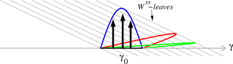
Figure 7: Geometry of folding in relation to the $W^{ss}$-foliation. Shown are a segment $\gamma_{0}\subset\gamma$, its image after one kick, and two of the subsequent images under the flow.

To develop a quantitative understanding of the factors conducive to the production of chaos, it is illuminating to consider the following linear shear model [46, 41]:

$$\begin{array}[]{rcl}\dot{\theta}&=&1+\sigma y\ ,\\ \dot{y}&=&-\lambda y+A\sin(2\pi\theta)\cdot\sum_{n=0}^{\infty}\delta(t-nT)\ .\end{array}$$ (7)

Here, $\theta\in{\mathbb{S}}^{1}$ and $y\in{\mathbb{R}}$ are phase variables, and $\sigma,\lambda,A$ are constants. We assume for definiteness that $\sigma$ and $\lambda$ are $>0$, so that when $A=0$, the system has a limit cycle $\gamma$ at $\{y=0\}$. Its $W^{ss}$-leaves are easily computed to be straight lines with slope $=-\frac{\lambda}{\sigma}$. When $A\neq 0$, the system is kicked periodically with period $T$. For this system, it has been shown that the shear ratio

$$\frac{\sigma}{\lambda}\cdot A\ \equiv\ \frac{\mbox{shear}}{\mbox{damping}}\cdot\mbox{deformation}\ =\ \frac{1}{|\mbox{slope}(W^{ss})|}\cdot\mbox{deformation}$$ (8)

is an excellent predictor of the dynamics of the system. Roughly speaking, if $\lambda_{\rm max}$ denotes the largest observed Lyapunov exponent, then

• if the shear ratio is sufficiently large, $\lambda_{\rm max}$ is likely to be $>0$;

• if the shear ratio is very small, then $\lambda_{\rm max}$ is slightly $<0$ or equal to $0$;

• as the shear ratio increases from small to large, $\lambda_{\rm max}$ first becomes negative, then becomes quite irregular (taking on both positive and negative values), and is eventually dominated by positive values.

To get an idea of why this should be the case, consider the composite kick-and-slide action in Fig. 7 in the context of Eq. (7). The time-$T$ map of Eq. (7) is easily computed to be

$$\begin{array}[]{rcl}\theta_{T}&=&\theta+T+\frac{\sigma}{\lambda}\cdot\big{[}A\sin(2\pi\theta)+y\big{]}\cdot\big{(}1-e^{-\lambda T}\big{)}\qquad\mbox{(mod 1)}\ ,\vspace{1.5ex}\\ y_{T}&=&e^{-\lambda T}\cdot\big{(}y+A\sin(2\pi\theta)\big{)}\ .\end{array}$$ (9)

When the contraction in $y$ is sufficiently strong, the first component of this map gives a good indication of what happens in the full $2$-D system. As an approximation, define $f_{T}(\theta)=\theta_{T}$ and view $f_{T}$ as a map of $\gamma$ to itself. When the shear ratio is large and $(1-e^{-\lambda T})$ is not too small, $|f_{T}^{\prime}|$ is quite large over much of $\gamma$, and the associated expansion has the potential to create the positive $\lambda_{\rm max}$ mentioned in (a). At the opposite extreme, when the shear ratio is very small, $f_{T}$ is a perturbation of the identity; this is the scenario in (b). Interestingly, it is for intermediate shear ratios that $f_{T}$ tends to have sinks, resulting in $\lambda_{\rm max}<0$ for the $2$-D system. The $1$-D map $f=\lim_{T\to\infty}f_{T}$ is known variously as the phase resetting curve or the singular limit. It is used heavily in [40, 41, 42, 43] to produce rigorous results for large $T$.

We now return to the the more general setting of $\varphi_{t}$ with discrete kicks $\kappa_{n}$, and try to interpret the results above as best we can. To make a meaningful comparison with the linear shear flow, we propose to first put our unforced system in “canonical coordinates,” i.e., to reparametrize the periodic orbit $\gamma$ so it has unit speed, and to make the kick directions perpendicular to $\gamma$ — assuming the kicks have well defined directions. In these new coordinates, sizes of vertical deformations make sense, as do the idea of damping and shear, even though these quantities and the angles between $W^{ss}$-manifolds and $\gamma$ all vary along $\gamma$. Time intervals between kicks may vary as well. The general geometric picture is thus a distorted version of the linear shear flow. We do not believe there is a simple formula to take the place of the shear ratio in this general setting; replacing the quantities $\sigma,\lambda$ and $A$ by their averages is not quite the right thing to do. We emphasize, however, that while system details affect the numerical values of $\lambda_{\rm max}$ and the amount of shear needed to produce $\lambda_{\rm max}>0$, the fact that the overall trends as described in (a)–(c) above are valid has been repeatedly demonstrated in simulation; see, e.g., [26].

Generalization to stochastic forcing

We now replace the discrete-time kicks in the discussion above by a directed (degenerate) continuous stochastic forcing, i.e. by a term of the form $V(x)dW_{t}$ where $V$ is a vector field and $dW_{t}$ is white noise. By Trotter’s product formula, the dynamics of the resulting stochastic flow can be approximated by a sequence of composite maps of the form $\varphi_{\Delta t}\circ\kappa_{\Delta t,\omega}$ where $\Delta t$ is a small time step, $\kappa_{\Delta t,\omega}$ are kick maps (of random sizes) in the direction of $V$, and $\varphi_{\Delta t}$ is the unforced flow. Most of the time, the maps $\kappa_{\Delta t,\omega}$ have negligible effects. This is especially the case if the size of $V$ is not too large and damping is present. Once in a while, however, a large deviation occurs, producing an effect similar to that of the discrete-time kicks at times $T_{n}$ described above. Cast in this light, we expect that the ideas above will continue to apply – albeit without the factors in the shear ratio being precisely defined.

We mention two of the differences between stochastic forcing and periodic, discrete kicks. Not surprisingly, stochastic forcing gives simpler dependence on parameters: $\lambda_{\rm max}$ varies smoothly, irregularities of the type in (c) above having been “averaged out”. Overall trends such as those in (a)–(c) tend to be unambiguous and more easily detected than for deterministic kicks. Second, unlike periodic kicks, very small forcing amplitudes can elicit chaotic behavior without $\frac{\sigma}{\lambda}$ being very large; this is attributed to the effects of large deviations.

Generalization to quasi-periodic flows

We have chosen to first introduce the ideas above in the context of limit cycles where the relevant geometric objects or quantities (such as $\sigma,\lambda$ and $W^{ss}$) are more easily extracted. These ideas apply in fact to flows on a torus that are roughly “quasi-periodic” – meaning that orbits may or may not be periodic but if they are, the periods are large – provided the forcing, stochastic or discrete, has a well-defined direction as discussed earlier. The main difference between the quasi-periodic setting and that of a limit cycle is that $W^{ss}$-leaves are generally not defined. A crucial observation made in [26] is that since folding occurs in finite time, what is relevant to the geometry of folding is not the usual $W^{ss}$-foliation (which takes into consideration the dynamics as $t\to\infty$) but finite-time strong stable foliations. Roughly speaking, a time-$t$ $W^{ss}$-leaf is a curve segment (or submanifold) that contracts in the first $t$ units of time. For the ideas above to apply, we must verify that time-$t$ $W^{ss}$-manifolds exist, have the characteristics of a large shear ratio, and that $t$ is large enough for the folding to actually occur. If these conditions are met, then one can expect shear-induced chaos to be present for the same reasons as before.

4.2 Phase-locking and unreliability in the two-cell model

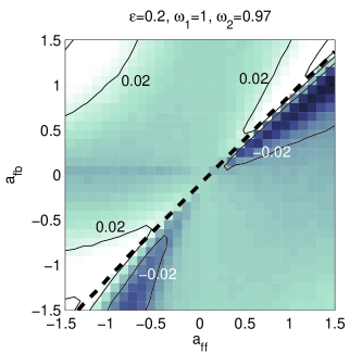
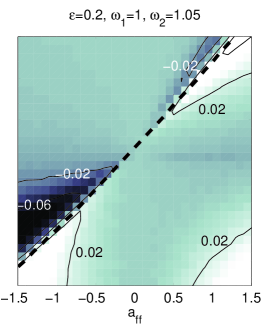
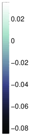
(a) $\varepsilon=0.2$

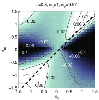
(b) $\varepsilon=0.8$

Figure 8: Maximum Lyapunov exponent $\lambda_{\rm max}$ versus coupling strengths in the two-cell network. In all plots, we use $\omega_{1}=1$. The $a_{\rm fb}^{*}$-curve from Fig. 4 is overlaid. All computed $\lambda_{\rm max}$ shown here have standard errors of $\leq 0.002$ as estimated by the method of batched means. By the Central Limit Theorem, this means the actual $\lambda_{\rm max}$ should lie within $\approx 2.5\times 0.002=0.005$ of the computed value with $\gtrsim 99\%$ probability. Remark on plots: We have chosen the dynamic range in shading the figures to allow meaningful comparison of figures; a side effect is that some contour lines may not be visible. We always indicate the actual range of values through explicit labels.

We now return to reliability questions of Eq. (2). In this subsection and the next, numerical data on $\lambda_{\rm max}$ as functions of $a_{\rm ff},a_{\rm fb}$ and $\varepsilon$ are discussed. Our aim is to identify the prominent features in these numerical results, and to propose explanations for the phenomena observed.

The present subsection is limited to phenomena related to the onset of phase-locking, which we have shown in Sect. 3.3 to occur at a curve in $(a_{\rm ff},a_{\rm fb})$-space that runs roughly along the diagonal. We will refer to this curve as the $a_{\rm fb}^{*}$-curve. Fig. 8 shows $\lambda_{\rm max}$ as a function of $a_{\rm ff}$ and $a_{\rm fb}$ for several choices of parameters, with $a_{\rm fb}^{*}$-curves from Fig. 4 overlaid for ease of reference. In the top two panels, where $\varepsilon$ is very small, evidence of events connected with the onset of phase-locking is undeniable: definitively reliable ($\lambda_{\rm max}<0$) and definitively unreliable ($\lambda_{\rm max}>0$) regions are both present. Continuing to focus on neighborhoods of the $a_{\rm fb}^{*}$-curves, we notice by comparing the top and bottom panels that for each $(a_{\rm ff},a_{\rm fb})$, the tendency is to shift in the direction of unreliability as $\varepsilon$ is increased. We will argue in the paragraphs to follow that these observations are entirely consistent with predictions from Sect. 4.1.

Shearing mechanisms

For concreteness, we consider the case $\omega_{2}>\omega_{1}$, and consider first parameters at which the unforced system has a limit cycle, i.e., for each $a_{\rm ff}\in[-1.5,1.5]$, we consider values of $a_{\rm fb}$ that are $>a_{\rm fb}^{*}$ and not too far from $a_{\rm fb}^{*}$. From Sect. 4.1, we learn that to determine the propensity of the system for shear-induced chaos, we need information on (i) the geometry of the limit cycle, (ii) the orientation of its $W^{ss}$-manifolds in relation to the cycle, and (iii) the effective deformation due to the forcing.

The answer to (i) is simple: As with all other trajectories, the limit cycle is linear with slope $\gtrsim 1$ outside of the two corridors $|\theta_{1}|<b$ and $|\theta_{2}|<b$, where it is bent; see Fig. 3. As for (ii) and (iii), we already know what happens in two special cases, namely when $a_{\rm ff}=0$ or $a_{\rm fb}=0$. As discussed in Sect. 3.2, when $a_{\rm fb}=0$, vertical circles are invariant under $\varphi_{t}$. Since $W^{ss}$-leaves are the only manifolds that are invariant, that means the $W^{ss}$-manifolds are vertical. We noted also that the forcing preserves these manifolds. In the language of Sect. 4.1, this means the forcing creates no variation transversal to $W^{ss}$-leaves: the ordering of points in this direction is preserved under the forcing. Hence shear-induced chaos is not possible here, and not likely for nearby parameters. A similar argument (which we leave to the reader) applies to the case $a_{\rm ff}=0$. From here on, we assume $a_{\rm ff},a_{\rm fb}$ are both away from $0$.

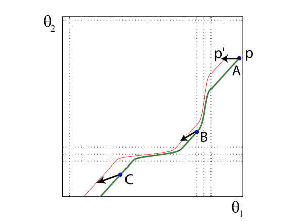
Figure 9: Rotation of vectors in backwards time. Here, $\omega_{1}=1,\omega_{2}=1.1,a_{\rm ff}=1,a_{\rm fb}=1.5$.

We now turn to a treatment of (ii) when $a_{\rm ff},a_{\rm fb}$ are both away from $0$, and claim that $W^{ss}$-leaves generally have a roughly diagonal orientation, i.e., they point in a roughly southwest-northeast (SW-NE) direction. To find this orientation, we fix a point $p$ on the limit cycle $\gamma$, and any nonzero tangent vector $v$ at $p$ (see Fig. 9). We then flow backwards in time, letting $p_{-t}=\varphi_{-t}(p)$ and $v_{-t}=D\varphi_{-t}(p)v$. The strong stable direction at $p_{-t}$ is the limiting direction of $v_{-t-n\tau}$ ($\tau=$ period of $\gamma$) as $n\to\infty$. Exact orientations of $W^{ss}$-leaves depend on $a_{\rm ff},a_{\rm fb}$ and are easily computed numerically.

The following simple analysis demonstrates how to deduce the general orientation of the $W^{ss}$-leaves in the two-oscillator system from the signs of its couplings. For definiteness, we consider $a_{\rm ff}>0$, so that $a_{\rm fb}^{*}$ is also positive and slightly larger than $a_{\rm ff}$. Here, a typical situation is that if we identify the phase space with the square $[0,1]\times[0,1]$, then the limit cycle crosses the right edge $\{1\}\times[0,1]$ in the bottom half, and the bottom edge $[0,1]\times\{0\}$ in the right half (as shown in Fig. 9). Let $A,B$ and $C$ be as shown, and consider a point $p$ at $A$. Flowing backwards, suppose it takes time $t_{B}$ to reach point $B$, and time $t_{C}$ to reach point $C$. We discuss how $v_{-t}$ changes as we go from $A$ to $C$. The rest of the time the flow is linear and $v_{-t}$ is unchanged.

From $A$ to $B$: Compare the backward orbits of $p$ and $p^{\prime}$, where $p^{\prime}=p+kv$ and $k>0$ is thought of as infinitesimally small. As these orbits reach the vertical strip $\{g>0\}$, both are bent downwards due to $a_{\rm ff}>0$. However, the orbit of $p^{\prime}$ is bent more because the function $z(\theta)$ peaks at $\theta=1/2$ (see Fig. 9). Thus, $v_{-t_{B}}=v+(0,-\delta_{1})$ for some $\delta_{1}>0$.

From $B$ to $C$: Continuing to flow backwards, we see by an analogous argument that as the two orbits cross the horizontal strip $\{g>0\}$, both are bent to the left, and the orbit of $p^{\prime}$ is bent more. Therefore, $v_{-t_{C}}=v_{-t_{B}}+(-\delta_{2},0)$ for some $\delta_{2}>0$.

Combining these two steps, we see that each time the orbit of $p_{-t}$ goes from $A$ to $C$, a vector of the form $(-\delta_{2},-\delta_{1})$ is added to $v_{-t}$. We conclude that as $t\to\infty$, the direction of $v_{-t}$ is asymptotically SW-NE. Moreover, it is a little more W than S compared to the limit cycle because $v_{-t}$ must remain on the same side of the cycle.

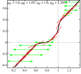
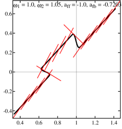
(a) $a_{\rm ff},a_{\rm fb}>0$		(b) $a_{\rm ff},a_{\rm fb}<0$

Figure 10: Strong stable directions along limit cycles. In (a), $a_{\rm fb}=a_{\rm fb}^{*}+0.1$; in (b), $a_{\rm fb}=a_{\rm fb}^{*}+0.2$. Additionally in (a), horizontal lines with arrows indicate the impact of the forcing at various points along the cycle; the variable impact is due to the $z$-function.

Numerical computations of strong stable directions are shown in Fig. 10. The plot in (a) is an example of the situation just discussed. The plot in (b) is for $a_{\rm ff},a_{\rm fb}<0$, for which a similar analysis can be carried out. Notice how small the angles are between the limit cycle and its $W^{ss}$-leaves; this is true for all the parameter sets we have examined where $a_{\rm fb}$ is close to $a_{\rm fb}^{*}$. Recall from Sect. 4.1 that it is, in fact, the angles in canonical coordinates that count. Since the limit cycle is roughly diagonal and the forcing is horizontal, putting the system in canonical coordinates will not change these angles by more than a moderate factor (except in one small region in picture (a)); i.e., the angles will remain small.

Finally, we come to (iii), the deformation due to the forcing. Given that the forcing is in the horizontal direction and its amplitude depends on $\theta_{1}$ (it is negligible when $\theta_{1}\approx 0$ and has maximal effect when $\theta_{1}\approx\frac{1}{2}$), it causes “bump-like” perturbations transversal to the $W^{ss}$-manifolds (which are roughly SW-NE) with a geometry similar to that in Fig. 7; see Fig. 10(a).

This completes our discussion of the limit cycle case. We move now to the other side of the $a_{\rm fb}^{*}$-curve, where the system is, for practical purposes, quasi-periodic (but not far from periodic). As discussed in the last part of Sect. 4.1, the ideas of shear-induced chaos continue to apply, with the role of $W^{ss}$-leaves now played by finite-time stable manifolds. Since these manifolds change slowly with $a_{\rm ff}$ and $a_{\rm fb}$, it can be expected – and we have checked – that they continue to make small angles with flowlines. Likewise, the forcing continues to deform flowlines by variable amounts as measured in distances transversal to finite-time stable manifolds.

We conclude that when $a_{\rm ff},a_{\rm fb}$ are both away from $0$, the geometry is favorable for shear-induced stretching and folding. Exactly how large a forcing amplitude is needed to produce a positive $\lambda_{\rm max}$ depends on system details. Such information cannot be deduced from the ideas reviewed in Sect. 4.1 alone.

Reliability–unreliability interpretations

We now examine more closely Fig. 8, and attempt to explain the reliability properties of those systems whose couplings lie in a neighborhood of the $a_{\rm fb}^{*}$-curve. The discussion below applies to $|a_{\rm ff}|>$ about $0.3$. We have observed earlier that for $a_{\rm ff}$ or $a_{\rm fb}$ too close to $0$, phase-space geometry prohibits unreliability.

Consider first Fig. 8(a), where the stimulus amplitude $\varepsilon=0.2$ is very weak. Regions showing positive and negative Lyapunov exponents are clearly visible in both panels. Which side of the $a_{\rm fb}^{*}$-curve corresponds to the phase-locked region is also readily recognizable to the trained eye (lower triangular region in the picture on the left and upper triangular region on the right; see Fig. 4).

We first explore the phase-locked side of the $a_{\rm fb}^{*}$-curve. Moving away from this curve, $\lambda_{\rm max}$ first becomes definitively negative. This is consistent with the increased damping noted in Sect. 3.2; see Fig. 6(b). As we move farther away from the $a_{\rm fb}^{*}$-curve still, $\lambda_{\rm max}$ increases and remains for a large region close to $0$. Intuitively, this is due to the fact that for these parameters the limit cycle is very robust. The damping is so strong that the forcing cannot (usually) push any part of the limit cycle any distance away from it before it is brought back to its original position. That is to say, the perturbations are negligible. With regard to the theory in Sect. 4.1, assuming $\sigma$ remains roughly constant, that $\lambda_{\rm max}$ should increase from negative to $0$ as we continue to move away from $a_{\rm fb}^{*}$ is consistent with increased damping; see (b) and (c) in the interpretation of the shear ratio.

Moving now to the other side of the $a_{\rm fb}^{*}$-curve, which is essentially quasi-periodic, regions of unreliability are clearly visible. These regions in fact begin slightly on the phase-locked side of the curve, where a weakly attractive limit cycle is present. We have presented evidence to support our contention that this is due to shear-induced chaos, or folding of the phase space. The fact that $\lambda_{\rm max}$ is more positive before the limit cycle is born than after can be attributed to the weaker-to-nonexistent damping before its birth. Thus the general progression of $\lambda_{\rm max}$ from roughly $0$ to definitively negative to positive as we cross the $a_{\rm fb}^{*}$-curve from the phase-locked side to the quasi-periodic side is altogether consistent with scenarios (a)–(c) in Sect. 4.1 together with the observations in the paragraph on stochastic forcing.

We point out that the unreliability seen in these panels is fairly delicate, perhaps even unexpected a priori for the smaller values of $a_{\rm ff}$ and $a_{\rm fb}$, such as $0.3<|a_{\rm ff}|,|a_{\rm fb}|<0.8$: The bending of the flow lines is rather mild at these smaller coupling parameters. Moreover, we know that no chaotic behavior is possible at $\varepsilon=0$, and the stimulus amplitude of $\varepsilon=0.2$ in the top panels is quite small. Recall, however, that the stimulus is a fluctuating white noise, and $\varepsilon$ gives only an indication of its average amplitude. As noted in Sect. 4.1, we believe the unreliability seen is brought about by an interaction between the large fluctuations in the stimulus presented and the shearing in the underlying dynamics.

In Fig. 8(b), the stimulus amplitude is increased to $\varepsilon=0.8$. A close examination of the plots shows that near to and on both sides of the $a_{\rm fb}^{*}$-curve, $\lambda_{\rm max}$ has increased for each parameter pair $(a_{\rm ff},a_{\rm fb})$, and that the reliable regions are pushed deeper into the phase-locked side compared to the top panels. This is consistent with the shear ratio increasing with forcing amplitude as predicted in Sect. 4.1.

This completes our discussion in relation to Fig. 8.

To complement the theoretical description of the geometry of folding given in Sect. 4.1, we believe it is instructive to see an actual instance of how such a fold is developed when the system (2) is subjected to an arbitrary realization of white noise. A few snapshots of the time evolution of the limit cycle under such a forcing is shown in Fig. 11. Notice that at the beginning, the combined action of the coupling and forcing causes the curve to wriggle left and right in an uncertain manner, but once a definitive kink is developed (such as at $t=3$), it is stretched by the shear as predicted.

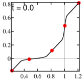
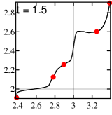
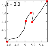
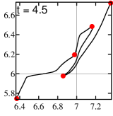
Figure 11: Folding action caused by white noise forcing and shear near the limit cycle (with $a_{\rm fb}>a_{\rm fb}^{*}$). At $t=0$, the curve shown is the lift of the limit cycle $\gamma$ to $\mathbb{R}^{2}$. The remaining panels show lifts of the images $F_{0,t,\omega}(\gamma)$ at increasing times. The parameters are $\omega_{1}=1$, $\omega_{2}=1.05$, $a_{\rm ff}=1$, $a_{\rm fb}=1.2$, and $\varepsilon=0.8$. Note that it is not difficult to find such a fold in simulations: very roughly, 1 out of 4 realizations of forcing gives such a sequence for $t\in[0,5]$.

4.3 Further observations on parameter dependence

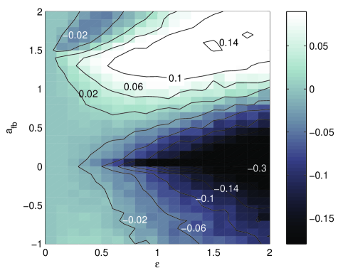
Figure 12: $\lambda_{\max}$ as function of $a_{\rm fb}$ and $\varepsilon$, with $\omega_{1}=1$, $\omega_{2}=1.1$, and $a_{\rm ff}=1$.

We now proceed to other observations on the dependence of $\lambda_{\rm max}$ on network parameters. Our aim is to identify the salient features in the reliability profile of the oscillator system (2) as a function of $a_{\rm ff},a_{\rm fb}$ and $\varepsilon$, and to attempt to explain the phenomena observed. Our observations are based on plots of the type in Figs. 8 and 12. Some of the explanations we venture below are partial and/or speculative; they will be so indicated.

1. Triple point: This phenomenon is the main topic of discussion in Sect. 4.2. Fig. 12 shows a different view of the parameter dependence of $\lambda_{\rm max}$. At about $a_{\rm fb}=1.4$, which is near $a_{\rm fb}^{*}$ for the parameters used, both positive and negative Lyapunov exponents are clearly visible for very small $\varepsilon$ in a manner that is consistent with Fig. 8 (even though the $\omega$’s differ slightly from that figure). We note again that this region, which we refer to as the “triple point,” is an area of extreme sensitivity for the system, in the sense that the system may respond in a definitively reliable or definitively unreliable way to stimuli of very small amplitudes, with the reliability of its response depending sensitively on coupling parameters.

2. Unreliability due to larger couplings: Fig. 8 and other plots not shown point to the occurrence of unreliability when $|a_{\rm ff}|$ and $|a_{\rm fb}|$ are both relatively large. We are referring here specifically to the “off-diagonal” regions of unreliability (far from the $a_{\rm fb}^{*}$-curve) in Fig. 8. This phenomenon may be partly responsible for the unreliability seen for the larger values of $a_{\rm ff}$ and $a_{\rm fb}$ on the diagonal as well; it is impossible to separate the effects of the different mechanisms.

   We do not have an explanation for why one should expect $\lambda_{\rm max}>0$ for larger $|a_{\rm ff}|$ and $|a_{\rm fb}|$ aside from the obvious, namely that tangent vectors are more strongly rotated as they cross the strips $\{|\theta_{i}|<b\}$, making it potentially easier for folding to occur. But folding does not occur at $\varepsilon=0$ in spite of this larger bending. We believe the difference between the two situations is due to the following noise-assisted mechanism: For $p\in{\mathbb{T}}^{2}$ and a tangent vector $u$ at $p$, let us say $u$ is positively oriented with respect to flowlines if starting from the direction of the flow and rotating counter-clockwise, one reaches $u$ before reaching the direction of the backward vector field. Without external forcing, if $u$ is positively oriented, $D\varphi_{t}(p)\cdot u$ will remain positively oriented for all $t$, because these vectors cannot cross flowlines. Now, in order for folding to occur, as in the formation of a horseshoe, the flow-maps must reverse the orientations of some tangent vectors. Even though larger values of $|a_{\rm ff}|$ and $|a_{\rm fb}|$ mean that tangent vectors are more strongly rotated, a complete reversal in direction cannot be accomplished without crossing flowlines. A small amount of noise makes this crossing feasible, opening the door (suddenly) to positive exponents.

3. The effects of increasing $\varepsilon$ (up to around $\varepsilon=2$):

   • Unreliable regions grow larger, and $\lambda_{\rm max}$ increases: A natural explanation here is that the stronger the stimulus, the greater its capacity to deform and fold the phase space – provided such folding is permitted by the underlying geometry. Because of the form of our stimulus, however, too large an amplitude simply pushes all phase points toward $\{\theta_{1}=0\}$. This will not lead to $\lambda_{\rm max}>0$, a fact supported by numerics (not shown).

   • Reliable regions grow larger, and the responses become more reliable: As $\varepsilon$ increases, the reliable region includes all parameters $(a_{\rm ff},a_{\rm fb})$ in a large wedge containing the $a_{\rm fb}=0$ axis. Moreover, in this region $\lambda_{\rm max}$ becomes significantly more negative as $\varepsilon$ increases. We propose the following heuristic explanation: In the case of a single oscillator, if we increase the amplitude of the stimulus, $\lambda_{\rm max}$ becomes more negative. This is because larger distortions of phase space geometry lead to more uneven derivatives of the flow-maps $F_{s,t;\omega}$, which in turn leads to a larger gap in Jensen’s Inequality (see the discussion before Prop. 2.1). For two oscillators coupled as Eq. (2), increasing $\varepsilon$ has a similar stabilizing effect on oscillator 1. Feedback kicks from oscillator 2 may destabilize it, as happens for certain parameters near the $a_{\rm fb}^{*}$-curve. However, if $a_{\rm ff}$ is large enough and enhanced by a large $\varepsilon$, it appears that the stabilizing effects will prevail.

5 Conclusions

We have shown that a network of two pulse-coupled phase oscillators can exhibit both reliable and unreliable responses to a white-noise stimulus, depending on the signs and strengths of network connections and the stimulus amplitude. Specifically:

1. (a) Dominantly feedforward networks are always reliable, and they become more reliable

   with increasing input amplitude.

   (b) Dominantly feedback networks are always neutral to weakly reliable.

2. When feedback and feedforward coupling strengths are comparable, whether both are negative (mutually inhibitory) or positive (mutually excitatory), we have observed the following:

   (a) For weak input amplitudes, the system is extremely sensitive to coupling strengths, with

   substantially reliable and unreliable configurations occurring in close proximity. This

   phenomenon is explained by mechanisms of phase locking and shear-induced chaos.

   (b) For stronger input amplitudes, the system is typically unreliable.

For weak stimuli, the most reliable configurations are, in fact, not dominantly feedforward but those with comparable feedforward–feedback couplings.

We expect these results to be fairly prototypical for certain pulse-coupled phase oscillators, such as those with “Type I” phase response curves that frequently occur in neuroscience. Understanding the effects of qualitatively different coupling types or oscillator models is an interesting topic for future study.

Another natural extension is to larger networks. This is the topic of the companion paper [25], where we use the present two-oscillator system as an embedded “module” to illustrate how unreliable dynamics can be generated locally and propagated to other parts of a network.

Acknowledgements: K.L. and E.S-B. hold NSF Math. Sci. Postdoctoral Fellowships and E.S-B. a Burroughs-Wellcome Fund Career Award at the Scientific Interface; L-S.Y. is supported by a grant from the NSF. We thank Brent Doiron, Bruce Knight, Alex Reyes, John Rinzel, and Anne-Marie Oswald for helpful discussions over the course of this project.

APPENDIX: Proof of Theorem 2

Here we prove the two lemmas needed for Theorem 2.

Let $\omega_{1},a_{\rm ff},\Delta\omega$ and $\Delta a_{\rm fb}$ be given, with $\Delta\omega,\Delta a_{\rm fb}>0$. To study the system where $\omega_{2}$ is defined by $\Delta\omega=1-\frac{\omega_{1}}{\omega_{2}}$ and $a_{\rm fb}=a_{\rm ff}+\Delta a_{\rm fb}$, we will seek to compare trajectories for systems with the following parameter sets:

$$\begin{array}[]{lllll}\mbox{System A}:&a_{\rm ff},&a_{\rm fb}=a_{\rm ff},&\omega_{1},&\omega_{2}=\omega_{1}\\ \mbox{System B}:&a_{\rm ff},&a_{\rm fb}=a_{\rm ff}&\omega_{1},&\omega_{2}=\omega_{1}+\Delta\omega\cdot\omega_{2}\\ \mbox{System C}:&a_{\rm ff},&a_{\rm fb}=a_{\rm ff}+\Delta a_{\rm fb},&\omega_{1},&\omega_{2}=\omega_{1}+\Delta\omega\cdot\omega_{2}\end{array}$$

That is, System C is the system of interest, and Systems A and B are used to help analyze System C. We introduce also the following notation: $H$ and $V$ denote the horizontal and vertical strips of width $2b$ centered at integer values of $\theta_{2}$ and $\theta_{1}$. We will work in $\mathbb{R}^{2}$ instead of $\mathbb{T}^{2}$.

Lemma 3.2: There exist $b_{1}$ and $K>0$ such that for all admissible $(\omega_{1},\omega_{2},a_{\rm ff},a_{\rm fb})$, if $b<b_{1}$ and $\Delta a_{\rm fb}<Kb^{-2}\Delta\omega$, then $T(1-b)<1-b$.

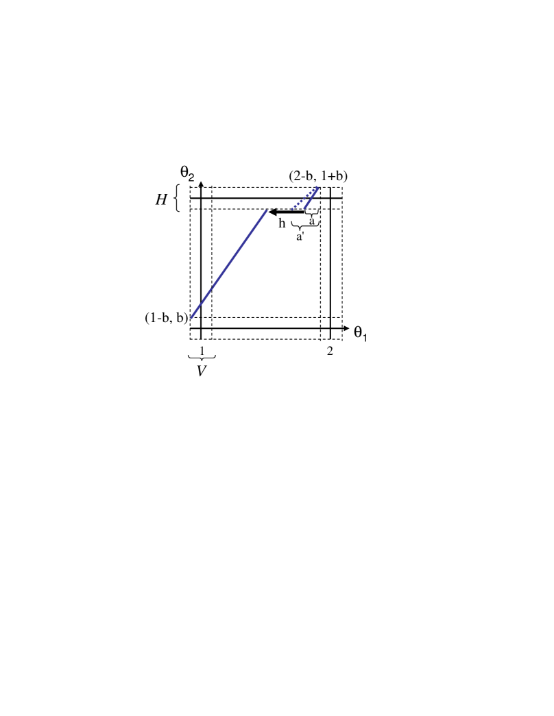
Figure 13: Values used in proving Lemma 3.2.

Proof.

For each of the 3 parameter sets above, two orbits are considered: Orbit 1 starts from $(\theta_{1},\theta_{2})=(1-b,b)\in\Sigma_{b}$ and runs forward in time until it meets $\Sigma_{1-b}=\{\theta_{2}=1-b\}$; orbit 2 starts from $(2-b,1+b)\in\Sigma_{1+b}$ and runs backward in time until it meets $\Sigma_{1-b}$. We need to prove that for System C, under the conditions in the lemma, the end point of orbit 1 lies to the left of the end point of orbit 2 (as shown in Fig. 13). This is equivalent to $T(1-b)<1-b$.

For System A, orbits 1 and 2 meet, since for this set of parameters, $T(x)=x$ for all $x$ as noted in Sect. 3.3. Comparing Systems A and B, since the vector field for System B has greater slope everywhere, and outside of $H\cup V$ it has slope $\frac{\omega_{2}}{\omega_{1}}>1$, we conclude that for System B the end point of orbit 1 lies to the left of the end point of orbit 2, with a separation $h>\Delta\omega/2$; see Fig. 13.

Next, we compare Systems B and C. Orbit 1 for the two systems is identical, since the equation outside of $H$ does not involve $a_{\rm fb}$. Orbit 2, however, differs for the two systems. To estimate by how much, we compare $a$, the distance from the end point of orbit 2 to $\theta_{1}=2$ for System B, and $a^{\prime}$, the corresponding distance for System C as marked in Fig. 13. First, there exist $b_{1}$ and $k_{1}>0$ such that for $\theta_{1}\in(2-5b_{1},2)$, we have $z(\theta_{1})<k_{1}(2-\theta_{1})^{2}$ and $|z^{\prime}(\theta_{1})|<2k_{1}(2-\theta_{1})$. Shrinking $b_{1}$ further if necessary, we have that for $b<b_{1}$, orbit 2 has slope $>1/2$ everywhere and therefore the entire orbit, for both Systems B and C, lies within the region $H\cap\{2-5b<\theta_{1}<2-b\}$. The next step is to apply Gronwall’s Lemma to a system that incorporates both Systems B and C. Since $\theta_{2}(t)$ is identical for the two systems in the relevant region, we may write the equations as

$$\dot{\theta_{1}} = -\omega_{1}-(a_{\rm ff}+\delta)z(\theta_{1})\hat{g}(t)$$

$$\dot{\delta} = 0\;\;,$$

where $\delta=0$ corresponds to System B, $\delta=\Delta a_{\rm fb}$ corresponds to System C, and $\hat{g}(t)=g(\theta_{2}(t))$. Notice that each trajectory reaches $\Sigma_{1-b}$ after a time $\tau=2b/\omega_{2}$.

Motivated by the observation that $z(\theta_{1})={\mathcal{O}}(b^{2})$ in the relevant rectangle, we rescale the variable $\delta$ by $\bar{\delta}=b^{2}\delta$, and define $\bar{z}(\theta_{1})=\frac{1}{b^{2}}z(\theta_{1})$. This gives

$$\dot{\theta_{1}} = -\omega_{1}-(b^{2}a_{\rm ff}+\bar{\delta})\bar{z}(\theta_{1})\hat{g}(t)$$ (10)

$$\dot{\bar{\delta}} = 0\;\;.$$ (11)

To find $a$, we solve (10)-(11) over the time interval $[0,\tau]$, starting from $(\theta_{1}(0),\bar{\delta}(0))=(1-b,0)$; to find $a^{\prime}$, we do the same, starting from $(1-b,b^{2}\Delta a_{\rm fb})$. Applying Gronwall’s Lemma gives $|a^{\prime}-a|<b^{2}\Delta a_{\rm fb}\exp(L\tau)$, where $L$ is the Lipschitz constant for the allied vector field. To estimate $L$, note that $|\hat{g}|={\cal{O}}(\frac{1}{b})$, $|\bar{z}|={\cal{O}}(1)$, and $|\bar{z}^{\prime}|={\cal{O}}(\frac{1}{b})$. This gives $L={\cal{O}}(1/b)$, and $\exp(L\tau)={\cal{O}}(1)$. Therefore, $|a^{\prime}-a|<k_{2}b^{2}\Delta a_{\rm fb}$ for some constant $k_{2}$. Note that this constant can be made independent of $\omega_{1},\omega_{2},a_{\rm ff}$ or $a_{\rm fb}$.

Recall from the first part of the proof that to obtain the desired result for System C, it suffices to guarantee $|a^{\prime}-a|<h$. This happens when

$$\Delta a_{\rm fb}<\frac{\Delta\omega}{2k_{2}b^{2}}:=Kb^{-2}\Delta\omega\;\;.$$ (12)

∎

Lemma 3.3: There exist $b_{2},C>0$ and $x_{1}\in(0,1-b)$ such that for all admissible $(\omega_{1},\omega_{2},a_{\rm ff},a_{\rm fb})$, if $b<b_{2}$ and $\Delta a_{\rm fb}>C\Delta\omega$, then $T(x_{1})>x_{1}$.

Proof.

All orbit segments considered in this proof run from $\Sigma_{b}\cap\{\theta_{1}\in(0,1)\}$ to $\Sigma_{1+b}$. We assume $a_{\rm ff}>0$; the case $a_{\rm ff}<0$ is similar. First, we fix $x_{0},x_{1}>b$ so that for all admissible $(\omega_{1},\omega_{2},a_{\rm ff},a_{\rm fb})$, the trajectory starting from $x_{1}$ intersects $H=\{1-b<\theta_{2}<1+b\}$ in $H\cap\{\theta_{1}\in(1+x_{0},\frac{3}{2})\}$. Such $x_{0},x_{1}$ clearly exist for small enough $b$. Starting from $x_{1}$, we compare the trajectories for Systems A, B and C. We know that the trajectory for System A will end in $(1+x_{1},1+b)$. Thus to prove the lemma, we need to show the trajectory for System C ends to the right of this point. This comparison is carried out in two steps:

Step 1: Comparing Systems A and B. We claim that the horizontal separation of the end points of these two trajectories is $<c\Delta\omega$ for some constant $c>0$. It is not a necessary assumption, but the comparison is simpler if we assume $b$ is small: First, a separation $c_{1}\Delta\omega$ in the $\theta_{2}$ direction develops between the trajectories as they flow linearly from $(x_{1},b)$ to $\theta_{1}=(1-b)$. Next, while the trajectories flow through $V$, Gronwall’s lemma can be used in a manner similar to the above to show they emerge from $V$ with a separation $\leq c_{2}\Delta\omega$ in the $\theta_{2}$ direction. Third is the region of linear flow, resulting in a separation $\leq c_{3}\Delta\omega$ in the $\theta_{1}$ direction as the trajectories enter $H$. Gronwall’s lemma’s is again used in the final stretch as the trajectories traverse $H$.

Step 2: Comparing Systems B and C. Notice that up until they reach $\Sigma_{1-b}$, the two trajectories are identical. In $H$, their $\theta_{2}$ coordinates are equal, and the crossing time is $\tau=\frac{2b}{\omega_{2}}$. Let $\theta_{1}^{B}(t)$ and $\theta_{1}^{C}(t),\ t\in[0,\tau]$, denote their $\theta_{1}$ coordinates while in $H$. We write

$$\theta_{1}^{C}(\tau)-\theta_{1}^{B}(\tau)\ =\ \int_{0}^{\tau}a_{\rm ff}(z(\theta_{1}^{C}(t))-z(\theta_{1}^{B}(t)))g(\theta_{2}(t))dt\ +\ \int_{0}^{\tau}\Delta a_{\rm fb}z(\theta_{1}^{C}(t))g(\theta_{2}(t))dt\ .$$

The first integral is $\geq 0$ by design: via our choice of $x_{1}$, we have arranged to have $1<\theta^{B}_{1}(t)<\theta_{1}^{C}(t)<\frac{3}{2}$, and the $z$-function is monotonically increasing between $\theta_{1}=1$ and $\theta_{1}=\frac{3}{2}$. As for the second integral, we know $z(\theta^{C}_{1}(t))$ is bounded away from $0$ since $1+x_{0}<\theta^{C}_{1}(t)<\frac{3}{2}$, so the integral is $>d\Delta a_{\rm fb}$ for some constant $d>0$. It follows that $T(x_{1})>x_{1}$ if $d\Delta a_{\rm fb}>c\Delta\omega$. ∎

References

- [1] L. Arnold. Random Dynamical Systems. Springer, New York, 2003.
- [2] P.H. Baxendale. Stability and equilibrium properties of stochastic flows of diffeomorphisms. In Progr. Probab. 27. Birkhauser, 1992.
- [3] E. Brown, P. Holmes, and J. Moehlis. Globally coupled oscillator networks. In E. Kaplan, J.E. Marsden, and K.R. Sreenivasan, editors, Problems and Perspectives in Nonlinear Science: A celebratory volume in honor of Lawrence Sirovich, pages 183–215. Springer, New York, 2003.
- [4] E. Brown, J. Moehlis, and P. Holmes. On the phase reduction and response dynamics of neural oscillator populations. Neural Comp., 16:673–715, 2004.
- [5] H.L. Bryant and J.P. Segundo. Spike initiation by transmembrane current: a white-noise analysis. Journal of Physiology, 260:279–314, 1976.
- [6] C.C. Chow. Phase-locking in weakly heterogeneous neuronal networks. Physica D, 118:343–370, 1998.
- [7] J.-P. Eckmann and D. Ruelle. Ergodic theory of chaos and strange attractors. Rev. Mod. Phys., 57:617–656, 1985.
- [8] G. B. Ermentrout. Type I membranes, phase resetting curves, and synchrony. Neural Comp., 8:979–1001, 1996.
- [9] G.B. Ermentrout. phase locking of weakly coupled oscillators. J. Math. Biol., 12:327–342, 1981.
- [10] G.B. Ermentrout and N. Kopell. Multiple pulse interactions and averaging in coupled neural oscillators. J. Math. Biol., 29:195–217, 1991.
- [11] Jean-Marc Fellous, Paul H. E. Tiesinga, Peter J. Thomas, and Terrence J. Sejnowski. Discovering spike patterns in neuronal responses. Journal of Neuroscience, 24(12):2989–3001, 2004.
- [12] Wulfram Gerstner, J. Leo van Hemmen, and Jack D. Cowan. What matters in neuronal locking? Neural Computation, 8(8):1653–1676, 1996.
- [13] D. Goldobin and A. Pikovsky. Synchronization and desynchronization of self-sustained oscillators by common noise. Phys. Rev. E, 71:045201–045204, 2005.
- [14] D. Goldobin and A. Pikovsky. Antireliability of noise-driven neurons. Phys. Rev. E, 73:061906–1 –061906–4, 2006.
- [15] J. Guckenheimer. Isochrons and phaseless sets. J. Math. Biol., 1:259–273, 1975.
- [16] B. Gutkin, G.B. Ermentrout, and M. Rudolph. Spike generating dynamics and the conditions for spike-time precision in cortical neurons. J. Computat. Neurosci., 15:91–103, 2003.
- [17] D. Hansel, G. Mato, and C. Meunier. Synchrony in excitatory neural networks. Neural Comp., 7:307–337, 1995.
- [18] A.V. Herz and J.J. Hopfield. Earthquake cycles and neural reverberations: collective oscillations in systems with pulse-coupled threshold elements. Phys. Rev. Lett., 75:1222–1225, 1995.
- [19] F.C. Hoppensteadt and E.M. Izhikevich. Weakly Connected Neural Networks. Springer-Verlag, New York, 1997.
- [20] Y. Le Jan. On isotropic Brownian motion. Z. Wahr. Verw. Geb., 70:609–620, 1985.
- [21] Yu. Kifer. Ergodic Theory of Random Transformations. Birkhauser, 1986.
- [22] E. Kosmidis and K. Pakdaman. Analysis of reliability in the Fitzhugh Nagumo neuron model. J. Comp. Neurosci., 14:5–22, 2003.
- [23] Y. Kuramoto. Phase- and center-manifold reductions for large populations of coupled oscillators with application to non-locally coupled systems. Int. J. Bif. Chaos, 7:789–805, 1997.
- [24] F. Ledrappier and L.-S. Young. Entropy formula for random transformations. Probab. Th. and Rel. Fields, 80:217–240, 1988.
- [25] K. Lin, E. Shea-Brown, and L-S. Young. Reliability of coupled oscillators II: Larger networks. submitted, 2007.
- [26] K. Lin and L.-S. Young. Shear-induced chaos. arXiv:0705.3294v1 [math.DS], 2007.
- [27] Z. Mainen and T. Sejnowski. Reliability of spike timing in neocortical neurons. Science, 268:1503–1506, 1995.
- [28] H. Nakao, K. Arai, K. Nagai, Y. Tsubo, and Y. Kuramoto. Synchrony of limit-cycle oscillators induced by random external impulses. Physical Review E, 72:026220–1 – 026220–13, 2005.
- [29] A.M. Nunes and Pereira. J.V. Phase-locking of two Andronov clocks with a general interaction. Phys. Lett. A, 107:362–366, 1985.
- [30] K. Pakdaman and D. Mestivier. External noise synchronizes forced oscillators. Phys. Rev. E, 64:030901–030904, 2001.
- [31] C.S. Peskin. Mathematical Aspects of Heart Physiology. Courant Institute of Mathematical Sciences, New York, 1988.
- [32] A. Pikovsky, M. Rosenblum, and J. Kurths. Synchronization: A Universal Concept in Nonlinear Sciences. Cambridge University Press, Cambridge, 2001.
- [33] J. Rinzel and G.B. Ermentrout. Analysis of neural excitability and oscillations. In C. Koch and I. Segev, editors, Methods in Neuronal Modeling, pages 251–291. MIT Press, 1998.
- [34] J. Ritt. Evaluation of entrainment of a nonlinear neural oscillator to white noise. Phys. Rev. E, 68:041915–041921, 2003.
- [35] S. Strogatz. From Kuramoto to Crawford: Exploring the onset of synchronization in populations of coupled oscillators. Physica D, 143:1–20, 2000.
- [36] S. Strogatz and R. Mirollo. Synchronization of pulse-coupled biological oscillators. SIAM Journal on Applied Mathematics, 50:1645 – 1662, 1990.
- [37] D. Taylor and P. Holmes. Simple models for excitable and oscillatory neural networks. J. Math. Biol., 37:419–446, 1998.
- [38] J. Teramae and T. Fukai. Reliability of temporal coding on pulse-coupled networks of oscillators. arXiv:0708.0862v1 [nlin.AO], 2007.
- [39] J. Teramae and D. Tanaka. Robustness of the noise-induced phase synchronization in a general class of limit cycle oscillators. Phys. Rev. Lett., 93:204103–204106, 2004.
- [40] Q. Wang and L.-S. Young. Strange attractors with one direction of instability. Comm. Math. Phys., 218:1–97, 2001.
- [41] Q. Wang and L.-S. Young. From invariant curves to strange attractors. Comm. Math. Phys., 225:275–304, 2002.
- [42] Q. Wang and L.-S. Young. Strange attractors in periodically-kicked limit cycles and Hopf bifurcations. Comm. Math. Phys., 240:509–529, 2003.
- [43] Q. Wang and L.-S. Young. Toward a theory of rank one attractors. Annals of Mathematics, to appear.
- [44] A. Winfree. Patterns of phase compromise in biological cycles. J. Math. Biol., 1:73–95, 1974.
- [45] A. Winfree. The Geometry of Biological Time. Springer, New York, 2001.
- [46] G. Zaslavsky. The simplest case of a strange attractor. Phys. Lett., 69A(3):145 147, 1978.
- [47] C. Zhou and J. Kurths. Noise-induced synchronization and coherence resonance of a Hodgkin-Huxley model of thermally sensitive neurons. Chaos, 13:401–409, 2003.