The Fourth Positive System of Carbon Monoxide in the Hubble Space Telescope Spectra of Comets

Abstract

The rich structure of the $A^{1}\Pi-X^{1}\Sigma^{+}$ system of carbon monoxide accounts for many of the spectral features seen in long slit $HST$-STIS observations of comets 153P/Ikeya-Zhang, C/2001 Q4 (NEAT), and C/2000 WM₁ (LINEAR), as well as in the $HST$-GHRS spectrum of comet C/1996 B2 (Hyakutake). A detailed CO fluorescence model is developed to derive the CO abundances in these comets by simultaneously fitting all of the observed $A-X$ bands. The model includes the latest values for the oscillator strengths and state parameters, and accounts for optical depth effects due to line overlap and self-absorption. A complete fitting of the CO spectral features using this model leads to the first identification of a molecular hydrogen line pumped by solar H I Lyman-$\beta$ longward of 1200 Å in the spectrum of comet 153P/Ikeya-Zhang. Pumping by strong solar lines also plays an important role in CO fluorescence, as shown by the detection in the spectrum of comet C/1996 B2 (Hyakutake) of bands from the (14-v″) and (9-v″) progressions pumped by solar H I Lyman-$\alpha$ and O I $\lambda$1302, respectively. Using spectra extracted at increasing distances from the comet nucleus or averaging over increasing effective apertures, the model fits yield radial profiles of CO column density that are consistent with a predominantly native source for all the comets observed by STIS. The derived CO production rates are $1.54\pm 0.09\times 10^{28}$ molecules s^-1 for 153P/Ikeya-Zhang, $1.76\pm 0.16\times 10^{28}$ molecules s^-1 for C/2001 Q4 (NEAT), and $3.56\pm 0.20\times 10^{26}$ molecules s^-1 for C/2000 WM₁ (LINEAR). In the absence of spatial information for comet C/1996 B2 (Hyakutake), we estimate a CO production rate of $4.97\pm 0.07\times 10^{28}$ molecules s^-1, assuming an entirely native source. The CO abundances relative to water in these comets span a wide range, from $0.44\pm 0.03$% for C/2000 WM₁ (LINEAR), $7.2\pm 0.4$% for 153P/Ikeya-Zhang, $8.8\pm 0.8$% for C/2001 Q4 (NEAT) to $20.9\pm 0.3$% for C/1996 B2 (Hyakutake). For comets C/2000 WM₁ and C/2001 Q4 we can compare these results with those derived from nearly simultaneous observations by the Far Ultraviolet Spectroscopic Explorer.

1. INTRODUCTION

Cometary ices have undergone little or no processing since their formation in the solar nebula and thus they represent an important clue in understanding the conditions in the early Solar System. However, this interpretation is complicated by the radial mixings in the protoplanetary disk and the dynamical evolution of comets, expelled to the outer Solar System from their original formation site. No pattern for the cometary composition and activity has emerged from the objects studied to date (Biver et al., 2002; Crovisier, 2007) and a larger sample is needed. The composition of cometary ices has been studied through spectroscopic observations or in situ measurements. In the analysis of cometary spectra it is important to establish whether the observed chemical species originate in the nucleus (native source) or in the coma (extended source). For this purpose, spatially-resolved observations are needed to derive the radial composition of the gas outflow.

Carbon monoxide (CO) is one of the most abundant molecules, whose mixing ratio relative to water varies greatly among comets (Biver et al., 2006; Bockelée-Morvan et al., 2004). As a highly volatile compound, with a sublimation temperature of 24 K, CO ice is thought to be a sensitive tracer of the temperature in the environment in which the comets formed. However, its origin as a native compound or a daughter product, and the correlation between the two sources is still not understood. Infrared observations of the CO ro-vibrational lines conclude that the CO source was mainly native in comet C/1996 B2 (Hyakutake) (DiSanti et al., 2003) and significantly extended for comet C/1995 O1 (Hale-Bopp) (Disanti et al., 2001). This paper complements previous findings with the first CO radial profiles constructed from ultraviolet spectra. Care must be taken in interpreting the brightness profiles, since saturation close to the nucleus could mimic the presence of an extended source. A comprehensive fluorescence model is developed to derive reliable CO column densities and estimate CO production rates from cometary spectra obtained by the Space Telescope Imaging Spectrograph (STIS) and the Goddard High Resolution Spectrograph (GHRS) on the Hubble Space Telescope (HST). Using the long-slit capabilities of the STIS instrument, this paper offers evidence that the native source of CO is dominant in three long period comets.

Table 1Comet observations.

Dataset	Date & Time	Exposure Time	rh	vh	$\Delta$	Instrument	Mode
	(UT)	(s)	(AU)	(km s-1)	(AU)
C/1996 B2 (Hyakutake)
Z35FN602T	1996-04-01 13:09:00	1305.600	0.885	–38.51	0.259	$HST$-GHRS	G140L;2.0
Z35FN604T	1996-04-01 13:39:00	217.600	0.885	–38.51	0.260	$HST$-GHRS	G140L;2.0
Z35FN702T	1996-04-01 14:44:00	1305.600	0.884	–38.53	0.262	$HST$-GHRS	G140L;2.0
Z35FN704T	1996-04-01 15:14:00	217.600	0.883	–38.53	0.262	$HST$-GHRS	G140L;2.0
C/2000 WM1 (LINEAR)
B0500301000	2001-12-07 08:50:00
to B0502401000	2001-12-10 06:48:00	36,467	1.120	–28.30	0.340	$FUSE$	LWRS
O6GR12010	2001-12-09 21:33:00	1800.194	1.085	–28.26	0.357	$HST$-STIS	G140L;52$\times$0.2
O6GR03010	2001-12-09 23:09:10	1440.197	1.084	–28.26	0.358	$HST$-STIS	G140L;52$\times$0.2
O6GR11010	2001-12-10 00:45:00	1800.198	1.083	–28.26	0.359	$HST$-STIS	G140L;52$\times$0.2
153P/Ikeya-Zhang
O8FY01010	2002-04-20 07:28:00	1800.199	0.887	29.07	0.426	$HST$-STIS	G140L;52$\times$0.2
O8FY02010	2002-04-20 10:40:00	1800.197	0.889	29.08	0.426	$HST$-STIS	G140L;52$\times$0.2
O8FY03010	2002-04-21 07:30:00	1440.197	0.904	29.15	0.422	$HST$-STIS	G140L;52$\times$0.2
C/2001 Q4 (NEAT)
E1390101000	2004-04-24 00:39:00
to E1390501000	2004-04-24 23:09:00	68,282	1.030	–10.80	0.510	$FUSE$	LWRS
O8VK04010	2004-04-25 20:03:00	1800.199	1.024	–10.26	0.473	$HST$-STIS	G140L;52$\times$0.2
O8VK01010	2004-04-26 00:49:00	1683.008	1.023	–10.18	0.468	$HST$-STIS	G140L;52$\times$0.2
O8VK07010	2004-04-30 00:51:00	1800.200	1.002	–8.37	0.386	$HST$-STIS	G140L;52$\times$0.2

CO ultraviolet fluorescence in cometary spectra was first detected during sounding rocket observations of comet West (C/1975 V1, Feldman & Brune, 1976) and has been subsequently observed by $IUE$ (Tozzi et al., 1998), $HST$ (Weaver, 1998), $FUSE$ (Feldman et al., 2002), the Hopkins Ultraviolet Telescope on the Astro-1 Space Shuttle mission (Feldman et al., 1991), and rockets (Woods et al., 1987; Sahnow et al., 1993; McPhate et al., 1999). The most important spectral features of CO in the ultraviolet (UV) are its electronic transitions belonging to the $A-X$, $B-X$ and $C-X$ systems, or to the forbidden Cameron bands. Fluorescence is the main emission mechanism for the $A^{1}\Pi-X^{1}\Sigma^{+}$ system (1300 – 1900 Å), $C^{1}\Sigma^{+}-X^{1}\Sigma^{+}$ system (0–0 band at 1087.9 Å), and $B^{1}\Sigma^{+}-X^{1}\Sigma^{+}$ system (0–0 band at 1150.5 Å). The Cameron bands, $a^{3}\Pi-X^{1}\Sigma^{+}$ (1900 – 2800 Å), are mainly excited by electron impact and photodissociation of CO₂ (Weaver et al., 1994). Although observations of the $A-X$ or Fourth Positive Group of CO in the UV spectra of comets have a long history, their interpretation has been difficult compared to that of the $B-X$ and $C-X$ systems at shorter wavelengths that have been observed more recently.

The spatial information offered by the high resolution long slit $HST$-STIS spectra of comets 153P/Ikeya-Zhang (C/2002 C1), C/2001 Q4 (NEAT), and C/2000 WM₁ (LINEAR) shows that close to the nucleus the CO emission in the $A-X$ system is self-absorbed. This follows from the observed change in the relative intensities in various vibrational progressions as the offset from the comet center increases (see § 3). Self-absorption makes it difficult to derive a reliable value for the CO column density in the absence of a model that takes into account optical depth effects.

A detailed model of the $A-X$ system is needed to track the effects of saturation and self-absorption. We constructed a database containing $\sim 10^{5}$ transitions between the first 50 rotational levels of each of the 37 vibrational levels of $X^{1}\Sigma^{+}$ and the 23 vibrational levels of $A^{1}\Pi$, taking into account the energy shifts and mixings of the transition probabilities due to interactions between the different parity sublevels (Le Floch et al., 1987; Morton & Noreau, 1989). Using a simple approximation for fluorescence in subordinate lines (Liu & Dalgarno, 1996), expanded with a comprehensive treatment of self-absorption, our model offers an excellent fit to the data. The $A-X$ fluorescence model is used to derive spatial profiles of the CO column density for the three comets observed by STIS. We find that the column density profiles are consistent with a dominant native source in all comets. The resulting production rates range between $3.56\times 10^{26}$ and $1.76\times 10^{28}$ molecules s^-1 and are corroborated by the results from high resolution $FUSE$ observations of C/2001 Q4 (NEAT) and C/2000 WM₁ (LINEAR) (Weaver et al., 2002). The $HST$-GHRS observations of comet C/1996 B2 (Hyakutake), a comet with a high CO production rate (Biver et al., 1999; DiSanti et al., 2003) and thus strongly affected by large optical depth effects, require the addition of geometrical corrections to the simple plane-parallel atmosphere model in order to reproduce the relative line strengths.

The $HST$ observations are described in § 2. Details about the model and its simplifying assumptions are found in § 3. Detailed data analysis follows in § 4, and a discussion of the results is given in § 5. We conclude with a summary in § 6.

2. OBSERVATIONS

The $HST$ observations are summarized in Table 1. Comets Ikeya-Zhang and C/2000 WM₁ (LINEAR) were observed near times of high solar activity, while C/2001 Q4 (NEAT) and Hyakutake were observed closer to solar minimum. The $HST$-STIS observations used the G140L grating and the 52X0.2 aperture (25″ $\times$ 0$\farcs$2 for L-mode MAMA), resulting in a spatial resolution of $\sim$0$\farcs$1 and a spectral resolution of $\sim$4 Å in the wavelength range 1150–1730 Å. The STIS instrument performance is described in Kimble et al. (1998) and Woodgate et al. (1998). The $HST$-GHRS (Heap et al., 1995) observations of comet C/1996 B2 (Hyakutake), covering the 1290–1590 Å bandpass with a spectral resolution of $\sim$4 Å, do not provide spatial information. The GHRS Large Science Aperture (LSA) translates into a 1$\farcs$74 $\times~{}$1$\farcs$74 post-COSTAR projected area. Given that $FUSE$ and $HST$-STIS observations of comets C/2000 WM₁ (LINEAR) and C/2001 Q4 (NEAT) were nearly simultaneous, we choose to include in Table 1 a summary of $FUSE$ observations for completeness (Feldman et al., 2002; Weaver et al., 2002).

3. FLUORESCENCE MODEL FOR THE $A^{1}\Pi$ – $X^{1}\Sigma^{+}$ SYSTEM OF CO

The Fourth Positive Group of CO, $A^{1}\Pi$ – $X^{1}\Sigma^{+}$, has non-negligible overlap integrals for most of the non-diagonal vibrational transitions. While for the $C-X$ and $B-X$ systems it is enough to model just the (0–0) and (1–0) bands, for the $A-X$ system we must take into account all bands connecting all 37 vibrational levels of the $X^{1}\Sigma^{+}$ state with all 23 vibrational levels of the $A^{1}\Pi$ state. Using only the first 50 rotational levels, which should be sufficient for typical physical conditions in cometary comae, the final database contains almost $10^{5}$ transitions. The latest values for the parameters of the $A^{1}\Pi$ (Kurucz, 1976; Morton & Noreau, 1989; Le Floch, 1991) and $X^{1}\Sigma^{+}$ states (George et al., 1994) were used to derive the energy levels and transition wavelengths. Following Morton & Noreau (1989), the rotational transition probabilities $A_{J\mbox{${}^{\prime}$}J\arcsec}$ were obtained from the band transition probabilities $A_{v\mbox{${}^{\prime}$}v^{\prime\prime}}$ (Beegle et al., 1999; Eidelsberg et al., 1999; Borges et al., 2001; Kirby & Cooper, 1989). Even though there are three rotational branches (P, Q and R, $\Delta J=0,\pm 1$) possible from the same rotational level of the $A^{1}\Pi$ state ($J^{\prime}$), due to the parity selection rule, the excitation rates and branching ratios for the P and R branches do not mix with those for the Q branch. Each $J\mbox{${}^{\prime}$}$ level of the $A^{1}\Pi$ state is split into 2 opposite parity sublevels ($\Lambda$-doubling) that have different energies and interactions with neighboring levels of other electronic states (Morton & Noreau, 1989). The energy level shifts and the changes in the lifetimes due to these interactions were taken into account when available (Morton & Noreau, 1989; Kittrell et al., 1993; Le Floch et al., 1987).

In a first approximation, the fluorescent emission in the Fourth Positive Group of CO is modeled following the prescription from Liu & Dalgarno (1996). This model successfully accounts for saturation in the absorption of the exciting radiation, using a Voigt profile with line overlap. A quick look at the data, however, shows that this approach only partially accounts for optical depth effects, and we must extend the model to include self-absorption in the fluorescent cascade. The STIS spectra of comet 153P/Ikeya-Zhang shown in Figure 1 are averaged over effective apertures of increasing size, centered on the comet nucleus. Self-absorption is easily recognized by noting that the bands connecting to the ground vibrational level (0–0, 1–0, 2–0, 3–0, 4–0, 5–0) show little decrease in brightness as we increase the integrated slit area and the average column density becomes lower, while the other bands from the progressions originating in the same upper level (see the unblended 0–1, 1–3, 2–2, 2–3, 4–1 and 5–1) decrease strongly in intensity, so that at low column densities the relative line ratios are in agreement with the optically thin limit.

Figure 1.— Spectra of comet 153P/Ikeya-Zhang extracted from apertures that are 1, 2, 4 and 6 arcseconds wide in the spatial direction, top to bottom, centered on the comet nucleus, showing the effects of self-absorption (see text). The strong features near 1564 Å and 1657 Å are emissions from atomic carbon.

The treatment of self-absorption is made under the assumption of local thermodynamic equilibrium (LTE), using the fact that the photon mean free path corresponds to an optical depth $\tau$ of one. Given that the gas temperature in the coma is less than 100 K for our observations, under LTE conditions we need only to take into account absorption out of the lowest (0) vibrational level of $X^{1}\Sigma^{+}$. Unlike for H₂ for example, the ro-vibrational levels of the ground state of CO have short lifetimes, making LTE a good approximation. The lines connecting to v″ = 0 for which $\tau$ at line center is greater than one are considered self-absorbed. Only an effective column density $N_{0}^{ij}=1/\sigma_{line-center}^{ij}$, smaller than the total absorbing column $N$, will contribute to the observed emission in a self-absorbed transition $i-j$. The excess brightness, due to absorption by the total column density $N$, is then redistributed among the optically thin lines originating in the same upper level $i$ according to the branching ratios, as seen in Figure 2.

Figure 2.— Illustration of the CO fluorescence model. The absorption profile for the $A-X$ (1-0) band is applied to the solar spectrum (upper panel) and the subsequent emission in the ($1-v\arcsec$) progression is shown before and after including self-absorption (middle and lower panels, respectively).

The model is constructed in the approximation of a uniform plane-parallel atmosphere. This approximation is of limited use, due to the spherical symmetry of the comet atmosphere and the Sun-comet-Earth geometry. The breakdown is more apparent for larger column densities, such as in the case of comet C/1996 B2 (Hyakutake), discussed in § 4.2. In the optically thin regime, valid at larger distances from the comet nucleus, as well as for unresolved objects, such geometrical effects are negligible. Introducing geometrical corrections in our model can be done by allowing the column density entering the absorption step to be different from the column density used for emission and self-absorption. This procedure accounts for the fact that the projected column density along the line-of-sight is larger than the column density towards the exciting radiation source. This difference leads both to the decrease in line saturation and to the enhancement of the optically thin lines versus the optically thick ones due to more self-absorption. The method is very robust, providing line intensities in agreement with the data.

4. DATA ANALYSIS

Although the brightness of the $A-X$ bands for the same comet should differ slightly from one observation to another due to varying comet heliocentric and geocentric distances, as well as due to possible periodic variations in the volatile vaporization rate, this variation is within the error bars of the observations and the use of an averaged STIS spectrum for each comet in order to improve the signal-to-noise ratio is warranted. We also select only the datasets that do not show significant deviations in background and intensity from one another.

High resolution solar spectra from the Ultraviolet Spectrometer Polarimeter Experiment on the Solar Maximum Mission (Tandberg-Hanssen et al., 1981) were used, scaled to match the solar activity at the time of comet observations as deduced from UARS/Solstice solar flux measurements (Rottman et al., 2001). The solar spectrum is shifted according to the comet motion relative to the Sun (Swings effect, Dymond et al., 1989). For the solar H I Lyman-$\alpha$ and -$\beta$ lines the SOHO/SUMER data of Lemaire et al. (2002) were used.

Table 2Model parameters.

Comet Name	$T_{\rm ROT}$	Doppler $b$ parameter	Solar Activity	$N_{\rm CO}$ Range
	(K)	(km s-1)		(1014 cm-2)
153P/Ikeya-Zhang	82	0.91	max	61.3–1.49
C/2001 Q4 (NEAT)	68	0.79	min	68.4–1.86
C/2000 WM1 (LINEAR)	77	0.72	max	0.935–0.327
C/1996 B2 (Hyakutake)	72	2.0	min	145

The only free parameter of the model is the column density, which is varied over a grid of values until the best fit is found. All model parameters used for each comet are summarized in Table 2. The values for the rotational temperature and Doppler $b$ parameter were chosen in agreement with infrared and radio measurements, when available. The Doppler $b$ parameter is given by $b=\sqrt{v_{therm}^{2}+v_{outflow}^{2}}\approx v_{outflow}$, where v_outflow is the source of non-thermal line broadening, and the thermal velocities are comparable to the uncertainties in v_outflow. Molecular lines of water and other molecules are well resolved by radio observations (usually to better than 0.1 km s^-1), and have a Gaussian profile, reflecting the symmetric outflow of the gas (Lecacheux et al., 2003; Wouterloot et al., 1998; Biver et al., 1999). Our observations have too low a resolution to be used to determine the Doppler line widths directly, so we rely on the published values for the expansion velocity of the gas, derived from the line profiles after correcting for thermal and instrumental broadening.

4.1. $HST$-STIS Observations

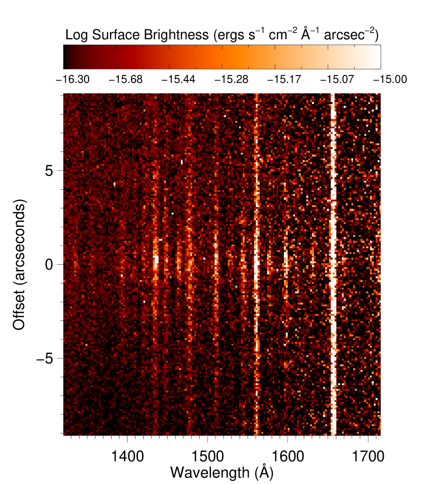
Figure 3.— $HST$-STIS spectral image of comet 153P/Ikeya-Zhang, showing the line brightness variation along the slit. The spectral region containing the strong geocoronal H I $\lambda$1216 and O I $\lambda$1302 has been excluded. The carbon multiplets at 1561.0 Å and 1657.6 Å are relatively constant due to the extended source component. The zero point in the vertical direction marks the location of the brightness peak, chosen as the center of our integration bins.

The high spatial resolution of the $HST$-STIS instrument is illustrated by the spectrum of comet 153P/Ikeya-Zhang in Figure 3. The CO $A-X$ lines form the majority of the observed features. Their intensity decreases rapidly along the slit, in contrast with the extended C I $\lambda$1561.0 and $\lambda$1657.6 multiplets. Using the spatial information available, we derive the CO spatial profile for each comet by fitting spectra extracted from regions of 1$\farcs$5 width at increasing offsets from the comet center. The selected regions sample areas of varying column density, for which our model estimates an average value. The comet nucleus is identified with the center of brightness, located at zero in Figure 3. The innermost region extracted, centered on the nucleus, is noisier due to the small integrated area. For intermediate regions the signal is better, due to the averaging of two regions, symmetric about the comet center. For each region, the background subtraction is performed by fitting a quadratic polynomial to selected points from feature-free intervals. These points were selected such that the outliers are discarded and the resulting polynomial fit is optimal.

The best-fit column density for each region and its standard deviation are derived by minimizing the $\chi^{2}$ statistics, taking into account the errors in background subtraction. The range of column densities obtained for each comet observed by STIS is listed in Table 2, together with the average value for comet C/1996 B2 (Hyakutake). The results are further compared with the Haser native source model (Haser, 1957; Opal & Carruthers, 1977), with an outflow velocity of $0.85~{}r_{\rm h}^{-0.5}$ km s^-1, where $r_{\rm h}$ is the comet-Sun distance in AU (Budzien et al., 1994; Biver et al., 1999), and a CO lifetime of $2\times 10^{5}$ s. We derive the CO production rate for each comet by a least squares fit of the Haser model to the radial column density profile. The native source model is integrated over rectangular regions matching the 1$\farcs$5 spectral extractions along the STIS slit. The resulting production rates and their magnitude relative to water are listed in Table 3.

4.1.1 153P/Ikeya-Zhang

The values for the rotational temperature and Doppler $b$ parameter are 82 K and 0.91 km s^-1 respectively, derived from infrared and radio measurements (Dello Russo et al., 2004; Biver et al., 2006). Spectra extracted from 1$\farcs$5 intervals were fitted using CO column densities ranging from 6.13$\times$10¹⁵ to 1.49$\times$10¹⁴ cm^-2, as shown in Figure 4. The data shown are obtained by averaging the first and third STIS observations (Table 1), and the best fit model is overplotted in red. The second observation was not included due to the background mismatch with the other two. The derived values for the CO column density in each region are represented by stars in Figure 5, plotted as a function of the distance from the comet nucleus. The error bars are given by the $1\sigma$ confidence level from the $\chi^{2}$ statistics. Fitting to this radial profile a native source model integrated over rectangular regions with the same coverage as the extracted spectra (Opal & Carruthers, 1977), we obtain a production rate of $1.54\pm 0.09\times 10^{28}$ molecules s^-1. The native source model for the derived production rate is shown as a continuous line in the same figure. The resulting CO production rate relative to water is about $7.2\pm 0.4\%$. The water production rate ($2.15\times 10^{29}$ molecules s^-1) was obtained from a vectorial model fit to an $HST$-STIS observation of the OH (0-0) band made on 2002 April 21 at 12:19 UT.

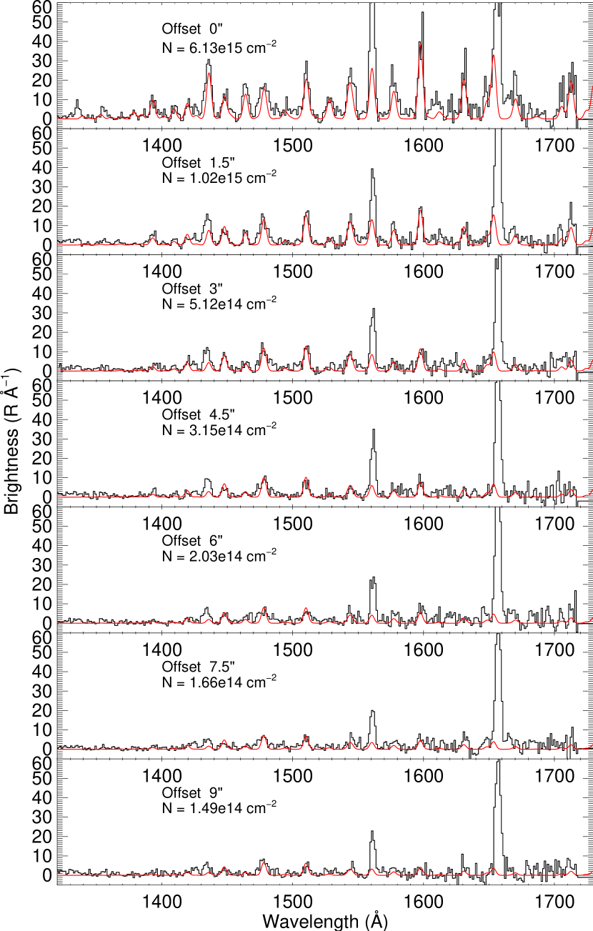
Figure 4.— $HST$-STIS spectra of comet 153P/Ikeya-Zhang extracted from 1.5″ intervals at increasing offsets from the center of brightness, assumed to be the location of the nucleus. The red line represents the model spectrum of the CO $A-X$ system for the best fit column density for each offset. The corresponding offsets and the best fit column densities are indicated on each panel. Other emission features belong to C II, C I, O I, S I, and H₂, as indicated in Figure 7.

Figure 5.— Spatial profile of the CO column density for comet 153P/Ikeya-Zhang. The stars with error bars represent the column density values derived from averaged spectra using the method presented in the text. The continuous line represents the column density profile predicted by the native source model when averaged over slits covering the same areas as the observations, with a production rate of 1.54$\times$10²⁸ molecules s^-1.

The residuals after subtracting the fluorescence spectrum for the CO $A-X$ system reflect the contributions of atomic species and allow the first detection of H₂ at wavelengths longward of 1200 Å. The H₂ spectrum consists of the P(1) lines of the Lyman (6-v″) progression pumped by solar H I Lyman-$\beta$. The H₂ lines with v″= 1–3 were first detected in the FUSE spectrum of comet C/2001 A2 (LINEAR) (Feldman et al., 2002). The lines at longer wavelengths, including the strongest one in the progression (v″= 13 at 1607.5 Å), remained undetected due to the abundance of CO features and lower resolution of the STIS instrument. The solar maximum value of flux, together with a velocity shift that placed the (6-0) P(1) line at the peak of the line, made it particularly fortuitous to detect the (6-13) P(1) line in comet Ikeya-Zhang. Figure 6 shows the shape and intensity of the solar Ly$\beta$ at minimum and maximum activity and the Doppler shifts of the H₂ absorption line corresponding to each comet. Although H₂ lines pumped by Ly$\beta$ were detected in comet C/2001 Q4 (Feldman et al., 2004), due to the large negative Doppler shift and the low solar activity, in the STIS bandpass the signal-to-noise for the H₂ lines is too low to warrant a detection. A comparison of the residuals for the two comets after subtracting the CO fluorescence model is shown in Figure 7. The STIS spectrum was integrated over a 4″ wide region centered on the comet nucleus, and the CO column density for the two comets ($N=3.07\times 10^{15}$ cm^-2 and $3.49\times 10^{15}$ cm^-2, respectively) has been obtained through the $\chi^{2}$ minimization procedure. The residuals for comets C/2000 WM1 and Hyakutake (not included in the figure) show no evidence for H₂, which can be explained by the large negative Doppler shifts with respect to the solar Ly$\beta$, the low outgassing rate of C/2000 WM1 and the minimum solar activity at the time of Hyakutake observations.

Figure 6.— Profile of solar Ly$\beta$ at maximum (August 2001) and minimum solar activity (July 1996). The velocity shifts of the absorbing H₂ (6–0) P1 line are shown for each comet.

The synthetic H₂ fluorescence spectra shown in red in Figure 7 are constructed under the assumption of an H₂O photodissociation source for H₂. According to the dissociation model, H₂ is rotationally hot (100-300 K) and its rotational levels are in statistical equilibrium, with an ortho/para ratio of 3, similar to water (Budzien et al., 1994; van Harrevelt & van Hemert, 2000; Bonev et al., 2007). The uncertainty in the exact value for the rotational temperature has little impact on the emerging spectrum, as the population of the J=1 level of the ground state does not differ significantly for rotational temperatures ranging from 100 to 300 K. The fluorescence efficiencies, or g-factors, used in the model were revised from those cited by Feldman et al. (2002), using the solar Lyman-$\beta$ profiles obtained over the past solar cycle by Lemaire et al. (2002), and accounting for the comet’s heliocentric velocity. The quality of the data does not warrant a $\chi^{2}$ fit for the H₂ fluorescence model, so we restrict ourselves to making rough estimates. Using an H₂ column density of $1.0\times 10^{14}$ cm^-2 at a rotational temperature of 200 K we obtain a reasonable agreement with the residuals for 153P/Ikeya-Zhang (Figure 7, upper panel). As was the case for comet C/2001 A2, this value for the H₂ column is consistent, within the rather large uncertainties in both the data and the models, with an H₂O photodissociation source. Constraining the H₂ production helps our understanding of this H₂O dissciation channel, for which little laboratory data is available.

Under our choice of parameters, the model for 153P/Ikeya-Zhang predicts about 5.5 R for the v″= 7,9 and 11 lines, at the level of the errors due to noise and CO subtraction, leaving only the (6–13) P(1) line detectable at a $\sim$3$\sigma$ level, with 18.4 R. This line is not detected in any other comet from our sample. For comparison, we model the H₂ fluorescence for comet C/2001 Q4. We use the same column density of H₂, as both C/2001 Q4 and 153P/Ikeya-Zhang have similar water production rates (see notes to Table 3). Due to the low solar activity and the unfavorable Doppler shift, the predicted line intensities are too low to be detected, consistent with the residuals (Figure 7, lower panel). The discrepancies between the H₂ models and the residuals are due to the uncertainties in the CO fluorescence model itself as well as to the noise in the data increasing towards longer wavelengths.

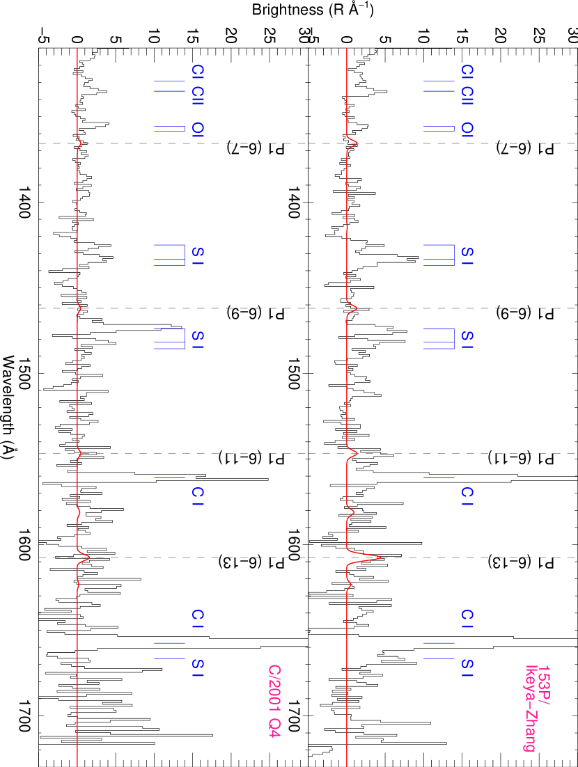
Figure 7.— Residuals from the spectrum of 153P/Ikeya-Zhang and C/2001 Q4 after subtracting the best fit CO model ($N=3.07\times 10^{15}$ cm^-2 and $3.49\times 10^{15}$ cm^-2, respectively). The comet spectra were extracted from a region of 4″ width, centered on the comet nucleus. The red line is the predicted H₂ fluorescence spectrum pumped by solar Lyman-$\beta$ for a column density of $1.0\times 10^{14}$ cm^-2 and a rotational temperature of 200 K. Other atomic contributions are shown in blue.

The strongest atomic lines seen in the residuals are also indicated in Figure 7. In addition to those lines usually seen in comets (McPhate et al., 1999), we also note the presence of the S I (${}^{1}\!D-^{1}\!D^{o}$) transition at 1666.7 Å. This transition is analogous to O I (${}^{1}\!D-^{1}\!D^{o}$) at 1152.2 Å (Feldman et al., 2002) and C I (${}^{1}\!D-^{1}\!P^{o}$) at 1930.9 Å (Tozzi et al., 1998). Using a g-factor of $1.92\times 10^{-5}$ photons atom^-1 s^-1 at 1 AU, the $\sim$30 rayleigh brightness corresponds to an average column density of S I ${}^{1}\!D$ atoms in the aperture of $1.24\times 10^{12}$ cm^-2. Since the lifetime of the metastable ${}^{1}\!D$ state of sulfur is only 28 s, this requires that within the aperture ${}^{1}\!D$ atoms be produced at a rate of $1.9\times 10^{26}$ s^-1 (0.09% relative to water). Collisional de-excitation of ${}^{1}\!D$ near the nucleus would raise this number. The likely source of these atoms is the photodissociation of sulfur-bearing molecules such as H₂S or CS₂, which must be produced at a rate greater than 0.1% relative to water.

4.1.2 C/2001 Q4 (NEAT)

Adjusting the model parameters to the conditions of NEAT Q4 observations we derive in the manner described for 153P/Ikeya-Zhang a CO production rate of $1.76\pm 0.16\times 10^{28}$ molecules s^-1, or $8.8\pm 0.8\%$ relative to water. For the water production rate, we derive a value of $2.0\times 10^{29}$ molecules s^-1 from STIS observations on 2004-04-23 21:39 UT. The CO model was fitted to the average of the first two STIS observations (Table 1). For the third observation the detector background level is much higher than for the other two. The adopted values for the rotational temperature and Doppler $b$ parameter are listed in Table 2. $FUSE$ observations of the CO $C-X$ Hopfield-Birge system at 1088 Å reveal a band profile consistent with a two component temperature model (Feldman et al., 2002). The hot component ($\sim$600 K) is believed to describe an extended CO source due to the dissociation of CO₂ (Feldman et al., 2006b). We use for our model the temperature of the cold component, estimated at $\sim$68 K, characteristic of the native CO source which dominates at the smaller cometocentric distances probed by STIS. Lacking direct radio measurements of the line widths, we use a value of 0.79 km s^-1 for the Doppler $b$ parameter, based on the outflow velocity 0.8$\times r_{\rm h}^{-0.5}$. The radial profile of the best-fit column densities and the native source model are plotted in Figure 8 as stars and continuous line, respectively.

Using a two-component fit to the CO $C-X$ band observed by $FUSE$ (Feldman et al., 2002) we derive CO column densities of $1.2\pm 0.3\times 10^{14}$ cm^-2 and $2.38\pm 0.08\times 10^{13}$ cm^-2 for the cold and hot component, respectively, averaged over the entire 30″ $\times$ 30″slit. A native source for the cold component requires a production rate of $1.36\pm 0.40\times 10^{28}$ molecules s^-1, or $6.8\pm 2.0\%$ relative to water. The solar flux pumping the $C-X$ fluorescence was based on quiet sun whole disk data from SOHO/SUMER (Curdt et al., 2001), normalized, at wavelengths longward of 1200 Å, to UARS/SOLSTICE solar flux measurements appropriate to the solar activity at the time of our observation (Rottman et al., 2001).

Figure 8.— Same as Figure 5, for comet C/2001 Q4 (NEAT). The production rate for the native source model was $1.76\times 10^{28}$ molecules s^-1.

4.1.3 C/2000 WM₁ (LINEAR)

The CO emission detected by STIS in the observation of comet C/2000 WM₁ (LINEAR) was too weak to allow us to repeat the same analysis performed in the case of comets 153P/Ikeya-Zhang and C/2001 Q4 (NEAT). Instead, we chose to integrate the STIS spectrum over increasing widths centered on the nucleus, in order to make use of the stronger signal in the center and to increase the number of contributing pixels. We started with a 4″ wide region which was increased progressively up to 16″. For the rotational temperature we used the 77 K value derived for the cold component using $FUSE$ observations (Weaver et al., 2002), while the Doppler $b$ parameter value of 0.72 km s^-1 was chosen to match the radio observations of Biver et al. (2006). All three STIS observations were averaged together to obtain detectable CO emission features. The best-fit column densities over the selected regions are plotted in Figure 9 as a function of the integrated slit width. Fitting a native source model integrated over the same rectangular regions we obtain a CO production rate of $3.56\pm 0.2\times 10^{26}$ molecules s^-1. This model is shown by a continuous line in Figure 9. A CO production rate of $0.44\pm 0.03$% relative to water is obtained adopting the favored H₂O production rate for the $FUSE$ observations (8.0$\times$10²⁸ molecules s^-1, Weaver et al., 2002). This makes C/2000 WM₁ (LINEAR) the most CO-poor comet of our sample.

Figure 9.— CO column density profile for comet C/2000 WM₁ (LINEAR) extracted from regions of increasing widths, centered on the comet nucleus. The continuous line corresponds to the values predicted by the native source model with a production rate of $3.56\times 10^{26}$ molecules s^-1, when integrated over similar slit sizes.

Table 3Production rates.

Comet Name	$Q_{\rm CO}$	$Q_{\rm CO}$/$Q_{\rm H_{2}O}$	Other $Q_{\rm CO}$ Measurements
	(1028 molecules s-1)	(%)	(1028 molecules s-1)
153P/Ikeya-Zhang	1.54 $\pm$ 0.09	7.2 $\pm$ 0.4	0.73 $\pm$ 0.16
C/2001 Q4 (NEAT)	1.76 $\pm$ 0.16	8.8 $\pm$ 0.8	1.36 $\pm$ 0.40
C/2000 WM1 (LINEAR)	0.036 $\pm$ 0.002	0.44 $\pm$ 0.03	0.035 $\pm$ 0.003
C/1996 B2 (Hyakutake)	4.97 $\pm$ 0.07	20.9 $\pm$ 0.3	4.84 $\pm$ 0.58

4.2. $HST$-GHRS Observations: C/1996 B2 (Hyakutake)

Since the $HST$-GHRS observations do not provide spatial information, we are unable to derive a CO column density profile for comet C/1996 B2 (Hyakutake). The CO production rate is obtained by comparing the CO column density derived by fitting our fluorescence model to the GHRS spectrum with the CO column density predicted for the GHRS aperture by the native source model. As model parameters for the synthetic spectrum we used a rotational temperature of 72 K given by the 63$\times r_{\rm h}^{-1.06}$ K dependence from DiSanti et al. (2003), which is similar to the value given by Lis et al. (1997), and a $b$ parameter of 2.0 km s^-1, within the range of outflow velocities measured by Wouterloot et al. (1998) but slighlty higher than derived from the optical line widths of Combi et al. (1999). A lower $b$ value is inconsistent with the total amount of absorbed solar radiation (from the conservation of the number of photons), suggesting larger turbulent motions in the 1$\farcs$74$\times$1$\farcs$74 area probed by GHRS.

Using the CO $A-X$ fluorescence model with self-absorption we obtain a first estimate for the CO column density averaged over the GHRS slit. However, the predicted line ratios are not in agreement with the data (see the red line in Figure 10, upper panel). In order to improve the fit and better constrain the column density we adjust the model to account for the geometry of the Sun-comet-Earth system. Starting with the previous estimate on the CO column we can constrain the ratio between the line-of-sight column density and the absorbing column on the comet-Sun direction. Iterating this procedure we obtain a best fit value for the line-of-sight CO column density of $1.45\pm 0.87\times 10^{16}$ cm^-2. This model is shown with a red line in the lower panel of Figure 10. The blue model in the same figure contains contributions from atomic species C II, C I, O I, and S I, as labeled, which account for the remaining features in the spectrum. Under the assumption of a native source model with the same lifetime and gas outflow velocity as employed for the STIS observations, we obtain a CO production rate of $4.97\pm 0.07\times 10^{28}$ molecules s^-1. This represents the highest CO production rate relative to water from our sample, $20.9\pm 0.3$%, using the water production rate of 2.38$\times$10²⁹ molecules s^-1 from Combi et al. (1998).

Figure 10 also clearly shows the presence of several bands originating on the v${}^{\prime}=9$ and 14 levels that are pumped by solar O I $\lambda$1302 and H I Lyman-$\alpha$, respectively (Wolven & Feldman, 1998). Kassal (1976) first pointed out that scattering of Lyman-$\alpha$ by the (14,0) band is comparable to, if not larger than, the direct solar scattering by all other bands of the CO Fourth Positive system for CO column densities $\geq 10^{17}$ cm^-2. The (14,4) band was subsequently identified in the spectrum of Venus (Durrance, 1981). These bands are not detected in any of the STIS comet spectra. The high column density in the field-of-view of comet Hyakutake makes them visible, albeit at low S/N, and allows for a determination of column density independent of optical saturation effects. In evaluating the fluorescence efficiency of these bands, the overlap between the solar lines and the individual lines of the CO bands is a sensitive function of rotational temperature and heliocentric velocity and requires accurate profiles of the solar lines (Lemaire et al., 2002). The (14-3), (14-4), and (9-2) bands are included in the model and are seen to be completely consistent with the CO column density derived above.

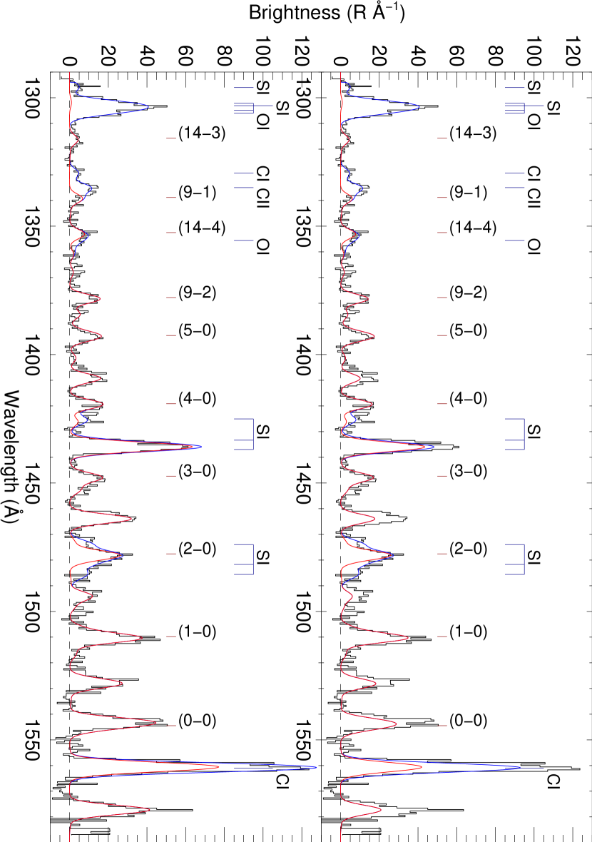
Figure 10.— $HST$-GHRS spectrum of comet C/1996 B2 (Hyakutake), and the model spectrum of the CO $A-X$ system for a line-of-sight column density of $1.45\times 10^{16}$ cm^-2, before (upper panel) and after geometric corrections (lower panel). The CO model spectrum is shown in red. The blue line contains contributions from atomic lines of C II, C I, O I, and S I, as indicated. The $A-X$ bands that do not change significantly due to the geometric effects are labeled.

We note that the optically thick bands connecting to the v″ = 0 level of the ground state, namely (1-0) at 1509.8 Å, (2-0) at 1477.6 Å, (3-0) at 1447.4 Å, (4-0) at 1419.1 Å and (5-0) at 1392.6 Å, all labeled in Figure 10, do not show a significant variation due to geometric corrections. This can be understood from the fact that while the correction adjusts the line-of-sight column density relative to the column absorbing the solar radiation, the emission in the optically thick lines will still be determined by the column corresponding to one optical depth, which depends only on temperature and $b$ parameter. The (0-0) band at 1544.5 Å does not seem to follow this pattern due to blending with the (3-2) band at 1542.5 Å. The same lack of variation is exhibited by the bands belonging to optically thin progressions pumped by solar emission lines, such as (14-3) at 1315.7 Å and (9-2) at 1377.8 Å. This is a result of the simple linear scaling in the optically thin limit, which makes the absorbing column indistinguishable from the emitting column.

5. DISCUSSION

5.1. Sources of Uncertainty and Comparison with Other Measurements

The derived column densities are subject to uncertainties due to the choice of model parameters and background subtraction. A more complete model would involve a multidimensional $\chi^{2}$ minimization to constrain simultaneously the column density, rotational temperature and Doppler $b$ parameter. Aside from the fact that this approach requires rather large computational resources, we expect that given the quality of the data the resulting $\chi^{2}$ 3D surfaces will have rather low contrast minima and the improvement in the resulting production rates would be negligible. More of a concern is the background subtraction in the $HST$-STIS data. The background is variable both in the spatial and spectral directions from one observation to another, making it impossible to give a comprehensive subtraction prescription. The optimal background subtraction is determined on a case-by-case basis. While the background-related uncertainties can lead to $\sim$30% variations in the values for the column densities, we estimate that the change in the resulting production rates is only about 6%. These values are only slightly larger than the $1\sigma$ error bars from the $\chi^{2}$ minimization. Similarly, increasing the rotational temperature from 70 K to 100 K results in a $\sim$30% decrease in production rate. However, the rotational temperatures relevant for our observations were derived from either $FUSE$ observations or from the T_rot vs. r_h dependences obtained by radio measurements, and are constrained to better than $\pm$6 K. This results only in a $\sim$7% variation in production rate, as the heliocentric distance of the comet does not vary significantly during our observations. The absolute values of the CO production rate and column density are also sensitive to the STIS calibration pipeline, which is based on point-source stellar standards. The column densities derived from STIS data could be overpredicted by at most 30% due to calibration offsets. Variations in the parameters used for the native source model, such as the CO lifetime and outlow velocity, could also change the production rate by a few percent. Other less quantifiable uncertainties to which the fluorescence model is particularly sensitive are the oscillator strengths and the UV solar flux, especially due to the variable emission features at high solar activity. Overall, we estimate that the systematic errors in the production rates amount to at most 15%.

To assess the effects of the error sources mentioned above, it is useful to compare our results to other measurements of the CO production rate in these comets from different spectral regions. The values obtained for comets C/2000 WM₁ (LINEAR) and C/1996 B2 (Hyakutake) are in excellent agreement with previous measurements. For comet C/1996 B2 (Hyakutake) at similar heliocentric distances Biver et al. (1999) find vales of $4.98\pm 0.09\times 10^{28}$ molecules s^-1 (0.952 AU) and $4.84\pm 0.58\times 10^{28}$ molecules s^-1 (0.894 AU). The production rate relative to water is comparable to previously measured mixing ratios of 14 to 19% (DiSanti et al., 2003) and 22% (Biver et al., 1999). For comet C/2000 WM₁ (LINEAR) both $FUSE$ (Weaver et al., 2002) and radio (Biver et al., 2006) observations are consistent with a CO mixing ratio of $\sim$0.4% and a CO production rate of $\sim$3 to 4$\times$10²⁶ molecules s^-1. A good agreement is again found when comparing the CO production rate derived for comet C/2001 Q4 (NEAT) with the results from $FUSE$ observations ($\S$ 4.1.2), listed in Table 3. We note that the measurements based on $FUSE$ observations used only the cold component of CO (see $\S$ 4.1.2) in estimating the CO production rate. The cold component is believed to reflect the native source of CO, which is directly probed by STIS. The two values agree marginally within the error bars, and the mismatch can be attributed to short time variability and pointing instability for the $FUSE$ observations. The count rates for the $C-X$ band in the $FUSE$ data show factor of two variations with a periodicity of $\sim$20 hours. The $FUSE$ observation overlaps with a much shorter STIS exposure, but the exact correlation in comet activity between the two datasets is hard to assess due to the different fields of view of the two instruments.

For comet 153P/Ikeya-Zhang the derived CO production rate is about a factor of 2 higher than the estimate from the range of values given by Biver et al. (2006) (using the $r_{\rm h}^{-2.1}$ scaling, see Table 3) and DiSanti et al. (2002). The factor of two difference may be attributed to the uncertainties in the model parameters (rotational temperature and Doppler parameter) and in the background subtraction. However, as discussed above, the combined sources of error should result in less than 15% uncertainty. On the other hand, the $r_{\rm h}^{-2.1}$ dependence was derived from two measurements, one at 0.51 AU and the other at 1.26 AU, not excluding the possibility of temporal variations affecting our observations at 0.89 AU. Moreover, the uncertainties in the $r_{\rm h}^{-2.1}$ scaling have not been quantified, making our value for the production rate more reliable. The CO abundance relative to water is again higher than other estimates. However, using the water production rate given by the 19.0$\times$10${}^{28}r_{\rm h}^{-4.}$ molecules s^-1 dependence derived by Biver et al. (2006) from H₂O observations made by the Odin satellite (Lecacheux et al., 2003), the CO mixing ratio decreases from $7.2\pm 0.4\%$ to $5.1\pm 0.3\%$. This would place the CO relative abundance in comet 153P/Ikeya-Zhang closer to the value of $3.8\pm 0.6\%$ at $\sim$1 AU (Biver et al., 2006) and $4.7\pm 0.8\%$ at 0.78 AU (DiSanti et al., 2002).

5.2. Application to Broad-band Imaging

The advantage of long-slit spectroscopy with STIS resides in giving us a better understanding of the spatial distribution of CO and the effects of increasing optical depths on the observed line ratios. We show how this information is applicable to broad-band imaging by integrating the brightness of the $A-X$ bands in the STIS bandpass that are not contaminated by atomic lines. We then integrate the fluorescence model over the same bands deriving an equivalent g-factor (as a ratio between the total brightness and the column density). Given the specific optical depth corrections in our model, the resulting g-factor will be in fact a brightness-column density dependence rather than a globally constant ratio. The radial brightness profile of the integrated bands observed by STIS can be then converted into a column density profile. This procedure can be visualized in Figure 11, where the data for comet 153P/Ikeya-Zhang have been used. The brightness profile has been rebinned in 1″ bins and background subtracted. The red histogram represents the column density profile obtained using the optically thick brightness-wavelength dependence, while the blue histogram represents the column density profile obtained in the optically thin approximation, using a constant g-factor. The black line is the native source model integrated in 1″ $\times$ 0$\farcs$2 bins, for a production rate of 1.54$\times$10²⁸ molecules s^-1, as derived in § 4.1.1. This figure illustrates the importance of including optical depth effects in order to predict the correct column density. This method has been used to interpret the imaging data from the HST Solar Blind Channel of the Advanced Camera for Surveys (ACS/SBC), and give an estimate of the number of molecules released from comet 9P/Tempel 1 as a result of the Deep Impact encounter (Feldman et al., 2006a). The uncertainties in this type of measurements come mainly from the additional emission features of atomic lines in the bandpass.

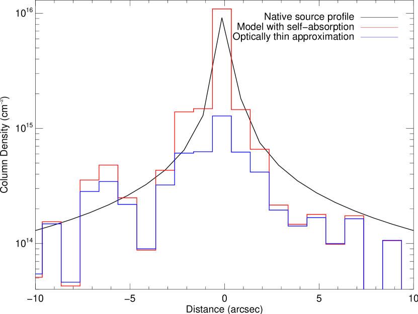
Figure 11.— Spatial profiles of the CO column density for comet 153P/Ikeya-Zhang, derived from the integrated brightness along the slit in 1″ bins, selecting the unblended lines from the $A-X$ system. The red line uses the total brightness-column density dependence associated with the present model, while the blue line is obtained in the optically thin approximation. The continuous black line is the native source model for a production rate of 1.54$\times$10²⁸ molecules s^-1, integrated in 1″ bins.

5.3. The Native Source of CO

The $HST$-STIS observations allow us to constrain the dominant source of CO in the region probed by the 25″ $\times$ 0$\farcs$2 slit. Reconstructing the surface column density distribution from the radial profile we estimate that in a 10″ $\times$ 10″ box the native source contribution to the total number of molecules is as high as 80% for comet C/2000 WM₁ (LINEAR) and from 90% to 99% for comets C/2001 Q4 (NEAT) and 153P/Ikeya-Zhang, respectively. This result suggests that the native source dominates in the inner $\sim 3000$ km from the comet center, while the extended component becomes important at larger distances. However, the native CO observed in the coma is linked to the amount of CO in the nucleus through the outgassing mechanism, which is not well known. Laboratory data suggests that the abundance of CO relative to water in the ice can be a factor of 5 to 10 lower than the one observed in the coma (Notesco et al., 1997; Colangeli et al., 2004). The exact value depends on the temperature at which the comet is outgassing.

The large variation in the CO production rate relative to water can be understood from the large range of heliocentric distances over which the comets have formed and then migrated to the outer parts of the Solar System through gravitational interactions with the planets. The observed diversity among comets is thought to be related to the local gas and dust composition and temperature where they formed. Under the assumption that CO has been trapped by water ice during comet formation, the local temperature can be estimated from the observed production rate (Notesco et al., 1997). The formation temperatures in our sample are expected to range from 50 K or less for comets C/2001 Q4, 153P/Ikeya-Zhang and Hyakutake, to more than 60 K for C/2000 WM₁. If the gas trapping mechanism is more efficient than deposition, as suggested by laboratory studies of CO and water interactions (Collings et al., 2003), important enrichments for the species with a higher sublimation temperature can occur (Notesco et al., 1997). This can explain the lack of correlation between the abundance of CO and that of other molecules with a similar sublimation temperature (Gibb et al., 2003; Biver et al., 2002).

6. SUMMARY

We have developed a fluorescence model for the interpretation of CO $A-X$ emission observed in several recent comets by the Hubble Space Telescope employing the latest values for the transition wavelengths and oscillator strengths. The radiative transfer approximation takes into account saturation effects using Voigt profiles for each of the $\sim$10⁵ transitions. Self-absorption is introduced using a photon mean free path approximation. This process is significant for column densities above few$\times$10¹⁴ cm^-2, encountered close to the comet nucleus. It is shown that the model reproduces the optically thin limit for lower column densities, at larger distances from the comet center. When the column densities are of the order $\sim$10¹⁶ cm^-2 or above, a good fit to the data requires a distinction between the absorbing CO column in the Sun-comet direction and the emitting column along the line-of-sight. The approximations in the radiative transfer model are justified for the quality of the available data. Constraining better the optical depth effects demands an exact treatment, which would be warranted at higher spectral resolution in order to predict the relative strengths of individual lines contained in the $A-X$ bands.

For the comets observed by STIS the fit of the column density profile is consistent with a predominantly native source, with production rates ranging from $3.56\times 10^{26}$ to $1.76\times 10^{28}$ molecules s^-1. The quality and the spatial extent of the STIS data does not allow for a detection of a small extended source component. We find large variations in the CO abundance relative to water, from 0.4% for C/2000 WM₁ (LINEAR) to 21% for C/1996 B2 (Hyakutake). This diversity among comets is still not well understood, as no clear trend emerges at the current stage of comet observations (Bockelée-Morvan et al., 2004). In spite of the caveats discussed in § 5, the absolute values of the CO production rate and column density are better constrained by the introduction of optical depth effects, and give reasonable confidence levels for the CO production rate and a good agreement with previous results. Moreover, the present model proves to be a valuable tool in analyzing broadband imaging data, such as the ACS/SBC observations of comet 9P/Tempel 1 (Feldman et al., 2006a).

References

- Beegle et al. (1999) Beegle, L. W., Ajello, J. M., James, G. K., Dziczek, D., & Alvarez, M. 1999, A&A, 347, 375
- Biver et al. (2002) Biver, N., et al. 2002, Earth Moon & Planets, 90, 323
- Biver et al. (1999) Biver, N., et al. 1999, AJ, 118, 1850
- Biver et al. (2006) Biver, N., et al. 2006, A&A, 449, 1255
- Bockelée-Morvan et al. (2004) Bockelée-Morvan, D., Crovisier, J., Mumma, M. J., & Weaver, H. A. 2004, in Comets II, ed. M. C. Festou, H. U. Keller, & H. A. Weaver (Tucson: Univ. Arizona Press)
- Bonev et al. (2007) Bonev, N., et al. 2007, ApJ, 661, L97
- Borges et al. (2001) Borges, I. J., Caridade, P. K. S. B., & Varandas, A. J. C. 2001, J. Mol. Spec., 209, 24
- Budzien et al. (1994) Budzien, S. A., Festou, M. C., & Feldman, P. D. 1994, Icarus, 107, 164
- Colangeli et al. (2004) Colangeli, L., Brucato, J. R., Bar-Nun, A., Hudson, R. L., & Moore, M. H. 2004, in Comets II, ed. M. C. Festou, H. U. Keller, & H. A. Weaver (Tucson: Univ. Arizona Press)
- Collings et al. (2003) Collings, M. P., Dever, J. W., Fraser, H. J., & McCoustra, M. R. S. 2003, Ap&SS, 285, 633
- Combi et al. (1999) Combi, M. R., Cochran, A. L., Cochran, W. D., Lambert, D. L., & Johns-Krull, C. M. 1999, ApJ, 512, 961
- Combi et al. (1998) Combi, M. R., Brown, M. E., Feldman, P. D., Keller, H. U., Meier, R. R., & Smyth, W. H. 1998, ApJ, 494, 816
- Crovisier (2007) Crovisier, J. 2007, in Proceedings of the XVIIIemes Rencontres de Blois: Planetary Science: Challenges and Discoveries, 28th May - 2nd June 2006, Blois, France, astro-ph/0703785
- Curdt et al. (2001) Curdt, W., Brekke, P., Feldman, U., Wilhelm, K., Dwivedi, B. N., Schühle, U., & Lemaire, P. 2001, A&A, 375, 591
- Dello Russo et al. (2004) Dello Russo, N., DiSanti, M. A., Magee-Sauer, K., Gibb, E. L., Mumma, M. J., Barber, R. J., & Tennyson, J. 2004, Icarus, 168, 186
- Disanti et al. (2001) Disanti, M. A., Mumma, M. J., Dello Russo, N., & Magee-Sauer, K. 2001, Icarus, 153, 361
- DiSanti et al. (2002) DiSanti, M. A., dello Russo, N., Magee-Sauer, K., Gibb, E. L., Reuter, D. C., & Mumma, M. J. 2002, in ESA SP-500: Asteroids, Comets, and Meteors: ACM 2002, ed. B. Warmbein, 571
- DiSanti et al. (2003) DiSanti, M. A., Mumma, M. J., Dello Russo, N., Magee-Sauer, K., & Griep, D. M. 2003, J. Geophys. Res., 108(E6), 5061
- Durrance (1981) Durrance, S. T. 1981, J. Geophys. Res., 86, 9115
- Dymond et al. (1989) Dymond, K. F., Feldman, P. D., & Woods, T. N. 1989, ApJ, 338, 1115
- Eidelsberg et al. (1999) Eidelsberg, M., Jolly, A., Lemaire, J. L., Tchang-Brillet, W. U., Breton, J., & Rostas, F. 1999, A&A, 364, 705
- Feldman (2005) Feldman, P. D. 2005, Physica Scripta, T119, 7
- Feldman & Brune (1976) Feldman, P. D., & Brune, W. H. 1976, ApJ, 209, L45
- Feldman et al. (1991) Feldman, P. D., et al. 1991, ApJ, 379, L37
- Feldman et al. (2006a) Feldman, P. D., Lupu, R. E., McCandliss, S. R., Weaver, H. A., A’Hearn, M. F., Belton, M. J. S., & Meech, K. J. 2006a, ApJ, 647, L61
- Feldman et al. (2006b) Feldman, P. D., McCandliss, S. R., & Weaver, H. A. 2006b, in AAS/Division for Planetary Sciences Meeting Abstracts, 20.06
- Feldman et al. (2002) Feldman, P. D., Weaver, H. A., & Burgh, E. B. 2002, ApJ, 576, L91
- Feldman et al. (2004) Feldman, P. D., et al. 2004, Bulletin of the American Astronomical Society, 36, 1121
- George et al. (1994) George, T., Urban, W., & Le Floch, A. 1994, J. Mol. Spec., 165, 500
- Gibb et al. (2003) Gibb, E. L., Mumma, M. J., dello Russo, N., Disanti, M. A., & Magee-Sauer, K. 2003, Icarus, 165, 391
- Haser (1957) Haser, L. 1957, Bull. Acad. R. Sci. Liège, 43, 740
- Heap et al. (1995) Heap, S. R., et al. 1995, PASP, 107, 871
- Huebner et al. (1992) Huebner, W. F., Keady, J. J., & Lyon, S. P. 1992, Solar photo rates for planetary atmospheres and atmospheric pollutants (Dordrecht: Kluwer Academic)
- Kassal (1976) Kassal, T. T. 1976, J. Geophys. Res., 81, 1411
- Kimble et al. (1998) Kimble, R. A., et al. 1998, ApJ, 492, L83
- Kirby & Cooper (1989) Kirby, K., & Cooper, D. L. 1989, J. Chem. Phys., 90, 4895
- Kittrell et al. (1993) Kittrell, C., Le Floch, A. C., & Garetz, B. A. 1993, J. Phys. Chem., 97, 2221
- Kurucz (1976) Kurucz, R. L. 1976, Smithsonian Astrophysical Observatory Special Report, 374
- Le Floch (1991) Le Floch, A. 1991, A&AS, 90, 513
- Le Floch et al. (1987) Le Floch, A., Launay, F., Rostas, J., Field, R. W., Brown, C. M., & Yoshino, K. 1987, J. Mol. Spec., 121, 337
- Lecacheux et al. (2003) Lecacheux, A., et al. 2003, A&A, 402, L55
- Lemaire et al. (2002) Lemaire, P., Emerich, C., Vial, J.-C., Curdt, W., Schühle, U., & Wilhelm, K. 2002, in ESA SP-508: From Solar Min to Max: Half a Solar Cycle with SOHO, ed. A. Wilson, 219
- Lis et al. (1997) Lis, D. C., et al. 1997, Icarus, 130, 355
- Liu & Dalgarno (1996) Liu, W., & Dalgarno, A. 1996, ApJ, 462, 502
- McPhate et al. (1999) McPhate, J. B., Feldman, P. D., McCandliss, S. R., & Burgh, E. B. 1999, ApJ, 521, 920
- Morton & Noreau (1989) Morton, D. C., & Noreau, L. 1989, ApJ, 347, 863
- Notesco et al. (1997) Notesco, G., Laufer, D., & Bar-Nun, A. 1997, Icarus, 125, 471
- Opal & Carruthers (1977) Opal, C. B., & Carruthers, G. R. 1977, ApJ, 211, 294
- Rottman et al. (2001) Rottman, G., Woods, T., Snow, M., & Detoma, G. 2001, Adv. Space Res., 27, 1927
- Sahnow et al. (1993) Sahnow, D. J., Feldman, P. D., McCandliss, S. R., & Martinez, M. E. 1993, Icarus, 101, 71
- Tandberg-Hanssen et al. (1981) Tandberg-Hanssen, E., et al. 1981, ApJ, 244, L127
- Tozzi et al. (1998) Tozzi, G. P., Feldman, P. D., & Festou, M. C. 1998, A&A, 330, 753
- van Harrevelt & van Hemert (2000) van Harrevelt, R. & van Hemert, M. C. 2000, J. Chem. Phys., 112, 5787
- Weaver (1998) Weaver, H. A. 1998, in ASP Conf. Ser. 143: The Scientific Impact of the Goddard High Resolution Spectrograph, ed. J. C. Brandt, T. B. Ake, & C. C. Petersen, 213
- Weaver et al. (2002) Weaver, H. A., Feldman, P. D., Combi, M. R., Krasnopolsky, V., Lisse, C. M., & Shemansky, D. E. 2002, ApJ, 576, L95
- Weaver et al. (1994) Weaver, H. A., Feldman, P. D., McPhate, J. B., A’Hearn, M. F., Arpigny, C., & Smith, T. E. 1994, ApJ, 422, 374
- Wolven & Feldman (1998) Wolven, B. C., & Feldman, P. D. 1998, in ASP Conf. Ser. 143: The Scientific Impact of the Goddard High Resolution Spectrograph, ed. J. C. Brandt, T. B. Ake, & C. C. Petersen, 373
- Woodgate et al. (1998) Woodgate, B. E., et al. 1998, PASP, 110, 1183
- Woods et al. (1987) Woods, T. N., Feldman, P. D., & Dymond, K. F. 1987, A&A, 187, 380
- Wouterloot et al. (1998) Wouterloot, J. G. A., Lingmann, A., Miller, M., Vowinkel, B., Winnewisser, G., & Wyrowski, F. 1998, Planet. Space Sci., 46, 579