Brane Decay and Defect Formation

Abstract

Topological defects are generically expected to form in models of brane inflation. Brane-anti-brane annihilation provides a way to gracefully end inflation, and the dynamics of the tachyon field results in defect formation. The formation of defects has been studied mainly from the brane world-volume point of view, but the defects are themselves lower-dimensional branes, and as a result they couple to bulk fields. To investigate the impact of bulk fields on brane defect formation, we construct a toy model that captures the essential features of the tachyon condensation with bulk fields. In this toy model, we study the structure of defects and simulate their formation and evolution on a lattice. We find that while bulk fields do not have a significant effect on defect formation, they drastically influence the subsequent evolution of the defects, as they re-introduce long-range interactions between them.

1 Introduction

Among the successes of the brane world model is the realization of the inflationary universe Dvali:1998pa . The brane-anti-brane separation plays the role of the inflaton and the non-zero attractive interaction generates the inflaton potential. Moduli stabilisation has been recently added to the brane-world model Kachru:2003sx , leading to even more realistic brane inflation models.

The brane inflation model contains a natural mechanism for ending inflation via the brane-anti-brane annihilation process Sen:1998sm . When the inter-brane separation decreases below a critical value, the tachyon field which corresponds to the open string stretching between the brane and the anti-brane develops an instability (Fig. 1), and the rolling of the tachyon field signals the decay of the brane-anti-brane pair. The tachyon field for a brane-anti-brane pair is a complex field and it has a non-trivial vacuum manifold which leads to the formation of topologically stable vortex configurations. These vortices are themselves lower-dimensional branes Kraus:2000nj ; Takayanagi:2000rz and their formation Jones:2003da and stability Copeland:2003bj have been studied for a variety of brane inflation models. These branes couple with bulk fields and would appear as cosmic strings to a 4-dimensional observer, therefore they are expected to provide a direct observational window into String Theory.

1.1 Brane-Anti-Brane Annihilation

The action for the tachyon field of a coincident brane-anti-brane pair has been computed in Kraus:2000nj ; Takayanagi:2000rz . Neglecting the gauge fields present in the brane and the anti-brane, the action has the form:

$$S=\int d^{p+1}x\sqrt{-g}e^{-T\overline{T}/2M_{s}^{2}}\left(1+\partial_{\mu}T\partial^{\mu}\overline{T}\right)$$ (1)

Performing a lattice evolution of the tachyon field Barnaby:2004dz , one notices that the field develops singularities [Fig. 1, right panel]. These singularities are the locations of the lower-dimensional branes formed in the brane annihilation process. In Kraus:2000nj ; Takayanagi:2000rz it was shown that a linear spatial tachyon profile reproduces the correct tension of the lower dimensional branes in the limit of infinite slope, so the occurrence of singularities was expected. One can use the lattice evolution of the tachyon field to estimate the density of vortices formed in brane annihilation, and the results suggest a much larger density than the one estimated via the Kibble mechanism Barnaby:2004dz . However, the occurrence of singularities does not allow one to study the evolution of the network of vortices.

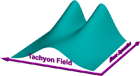
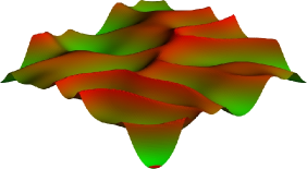
Figure 1: Left: The potential of the tachyon field as a function of the inter-brane separation. Right: The configuration of the rolling tachyon field during the brane-anti-brane annihilation process.

1.2 Coupling to Bulk fields

To obtain a more complete picture of the tachyon vortex formation we have to include the effects of all the fields involved. The tachyon field is charged under a linear combination of brane world-volume gauge fields and this same linear combination couples to a bulk antisymmetric tensor fields via a Chern-Simons (CS) term. The relevant terms in the action are Kraus:2000nj ; Takayanagi:2000rz :

$$S=\frac{1}{2\kappa_{10}^{2}}\int\sqrt{-G}\>d^{10}x\left[e^{-2\phi}\left(R+2\nabla\phi^{2}\right)-\frac{F_{p}^{2}}{2p!}\right]+2\pi\alpha^{\prime}T_{Dp}\int C_{p-1}\wedge\left(F^{+}-F^{-}\right)$$

$$-2T_{Dp}\int d^{p+1}x\,e^{-\phi}\,e^{-2\pi\alpha^{\prime}T\overline{T}}\biggl{[}1+8\pi\alpha^{\prime}\ln\left(2\right)D^{\mu}\overline{T}D_{\mu}T+\frac{\gamma{\alpha^{\prime}}^{2}}{8}\left(F^{+}_{\mu\nu}-F^{-}_{\mu\nu}\right)^{2}\biggr{]}$$

We want to study the formation and evolution of the tachyon vortices using the full non-linear equations of motion. Since the above action is 10-dimensional, we will first build a lower-dimensional toy model that captures the main features of the full 10-dimensional model and is amenable to study via a lattice simulation. We study the formation of vortices, so the minimal dimensionality of a brane that allows vortices to form is 2. We choose the bulk to also have the minimum possible dimensionality, 3, and replace the tachyon with a Higgs field in order to avoid singularities. The rest of the correspondence between the full and the toy model is presented in Table 1.

	10 D Model	Toy Model
brane dim.	$p+1$	$2+1$
bulk dim.	$9+1$	$3+1$
scalar field	tachyon, $\;T$	Higgs, $\;\phi$
vector field	$A_{\mu}^{+}-A_{\mu}^{-}$	$A_{\mu}$
tensor field	$C_{M_{1}\dots M_{p-1}}$	$C_{M}$
gravity	$G_{MN}$	flat space
coupling strength	dilaton, $\;\phi$	fixed coupling
potential	$e^{-\left|T\right|^{2}}$	$\lambda\left(\left|\phi\right|^{2}-\eta^{2}/2\right)^{2}$

Table 1: The correspondence between the full 10-dimensional model and the toy model

The action for the toy model follows that of the 10-dimensional model:

$${\mathcal{L}}=-\int_{{\mathcal{M}}_{3}}\!\!\!dx^{2}dt\left[\frac{F^{2}}{4g_{\rm brane}^{2}}+D_{\mu}\phi D^{\mu}\phi^{*}+V\left(\phi\right)\right]-\frac{c_{cs}}{2}\int_{{\mathcal{M}}_{3}}\!\!\!F\wedge C-\int_{{\mathcal{M}}_{4}}\!\!\!dx^{3}dt\frac{H^{2}}{4g_{\rm bulk}^{2}}$$

The details of the lattice regularisation of the above action are presented in Moore:2006ec . The important results are presented in Fig. 2 and 3. Reducing the size of the extra dimension forces the bulk field to have a larger gradient along the extra dimension, therefore increasing the total energy of the defect-anti-defect pair. The most dramatic effect is that of changing the strength of the CS coupling. Increasing the coupling reduces the quantum of brane gauge field magnetic flux trapped at the core of the defect, at large values of the coupling the flux being almost completely eliminated. This can be understood by first performing a dimensional reduction to 2 dimensions and then writing the equation of motion for the bulk field. The bulk field is sourced by the magnetic flux of the brane gauge field and this magnetic flux is localised at the defect core.

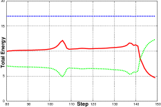
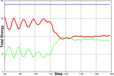
Figure 2: Effect of the size of the extra dimension on the energy of a defect pair. Left panel: the extra dimension is large and the bulk is effectively 3-dimensional. Right panel: the extra dimension is comparable to the size of the defect core, making the model effectively 2-dimensional. This also changes the strength of the interaction between the vortices, which annihilate faster when the extra dimension is small.

$$\nabla^{2}C^{0}=c_{\rm cs}g^{2}_{\rm bulk}F_{12}/2\pi R$$ (2)

We can use the solution for $C^{0}$ to find the energy density of the fields away from the defect core.

$${\mathcal{E}}=|D_{\theta}\phi|^{2}+\frac{2\pi R}{2g_{\rm bulk}^{2}}|\nabla C^{0}|^{2}$$

where $D_{\theta}\phi=(in/\rho-iA_{\theta})\phi$, $\phi^{*}\phi=v^{2}/2$, $A_{\theta}=\Phi/2\pi\rho$ and $C^{0}(\rho)=\frac{c_{\rm cs}g^{2}_{\rm bulk}}{2\pi R}\frac{\Phi}{2\pi}\ln(\rho/\rho_{0})$. $\Phi$ is the brane gauge field magnetic flux. Minimising the energy density with respect to $\Phi$ gives the results:

$${\mathcal{E}}=\frac{v^{2}n^{2}}{2\rho^{2}}\frac{a}{1+a}\,,\qquad\Phi=\frac{2\pi n}{1+a}\,,\qquad a\equiv\frac{c_{\rm cs}^{2}g_{\rm bulk}^{2}}{2\pi Rv^{2}}\,.$$

As the CS coupling is increased the magnetic flux unit at the defect core decreases and the energy of the defect interpolates smoothly between that of a local and that of a global defect. The bulk field also re-introduces long-range interactions between the local vortices.

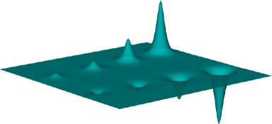
Figure 3: The magnetic flux at the core of the defect as a function of the CS coupling. The larger the coupling, the smaller the flux.

References

- (1) G. R. Dvali and S. H. H. Tye, Phys. Lett. B 450 (1999) 72
- (2) S. Kachru, et. al. JCAP 0310, 013 (2003)
- (3) A. Sen, JHEP 9808, 012 (1998)
- (4) P. Kraus and F. Larsen, Phys. Rev. D 63, 106004 (2001),
- (5) T. Takayanagi, S. Terashima and T. Uesugi, JHEP 0103, 019 (2001)
- (6) N. T. Jones, H. Stoica and S. H. H. Tye, Phys. Lett. B 563, 6 (2003)
- (7) E. J. Copeland, R. C. Myers and J. Polchinski, JHEP 0406, 013 (2004)
- (8) N. Barnaby, A. Berndsen, J. M. Cline and H. Stoica, JHEP 0506, 075 (2005)
- (9) G. D. Moore and H. Stoica, Phys. Rev. D 74, 065003 (2006)