ORBITAL INSTABILITIES
IN A TRIAXIAL CUSP POTENTIAL

Abstract

This paper constructs an analytic form for a triaxial potential that describes the dynamics of a wide variety of astrophysical systems, including the inner portions of dark matter halos, the central regions of galactic bulges, and young embedded star clusters. Specifically, this potential results from a density profile of the form $\rho(m)\propto m^{-1}$, where the radial coordinate is generalized to triaxial form so that $m^{2}=x^{2}/a^{2}+y^{2}/b^{2}+z^{2}/c^{2}$. Using the resulting analytic form of the potential, and the corresponding force laws, we construct orbit solutions and show that a robust orbit instability exists in these systems. For orbits initially confined to any of the three principal planes, the motion in the perpendicular direction can be unstable. We discuss the range of parameter space for which these orbits are unstable, find the growth rates and saturation levels of the instability, and develop a set of analytic model equations that elucidate the essential physics of the instability mechanism. This orbit instability has a large number of astrophysical implications and applications, including understanding the formation of dark matter halos, the structure of galactic bulges, the survival of tidal streams, and the early evolution of embedded star clusters.

1 INTRODUCTION

Many types of astrophysical objects are essentially collisionless systems with extended mass distributions, including dark matter halos, elliptical galaxies, galactic bulges, and star clusters. Although many of these systems display triaxial shapes, explicit analytic models for the gravitational potentials, force laws, and orbits of the triaxial incarnations of these systems are rare. This paper constructs an analytic form for the triaxial potential of an important class of systems, namely those in which the density profile approaches the form $\rho\sim 1/r$ in the spherical limit. With the potential in hand, we find the corresponding force terms (see also Poon & Merritt 2001; hereafter PM01) and study the orbits allowed by this triaxial system. One contribution of this present work is the discovery of a robust instability, wherein the orbital motion initially confined to any of the three principal planes can be unstable to the growth of the amplitude of the motion in the perpendicular direction. In addition to establishing the existence of the instability, this paper develops a set of model equations that allow for a (mostly) analytic description of the instability, the magnitude of the growth rate, and the saturation mechanism.

This particular form for the density profile $\rho\sim 1/r$ arises in many contexts. The Hernquist density profile, which has this form in the inner limit (Hernquist 1990), was originally constructed to describe the $R^{1/4}$ law in galactic bulges and elliptical galaxies. Since the Hernquist profile arises in many other contexts, we previously studied orbital solutions in the full (spherical) Hernquist potential and obtained a number of analytic results that are applicable to the present analysis (Adams & Bloch 2005, hereafter AB05). However, these bulge systems are known to be triaxial (Binney & Tremaine 1987, hereafter BT87; Binney & Merrifield 1998), and hence the triaxial generalization of the potential is important for understanding these galactic-scale systems. For example, triaxial potentials support box orbits, which allow stars to wander arbitrarily close to the galactic center; this behavior affects the rate at which stars interact with the central black hole.

On a larger scale, numerical simulations indicate that the density profiles of dark matter halos display a nearly universal form in which $\rho\sim 1/r$ in the inner regime (Navarro et al. 1997, hereafter NFW). Recent numerical simulations that carry the calculations into the future (Busha et al. 2005) show that the asymptotic form of the density profile becomes steeper at large radii and is well-described by a Hernquist profile (Hernquist 1990) but maintains the same $\rho\sim 1/r$ form on the inside. Additional studies suggest that this result for the inner form is robust; if the density profile is written in the form $\rho\propto r^{-p}$, then $p\leq 1.2$ (see Diemand et al. 2004, Hayashi & Navarro 2006, Huss et al. 1999, and references therein). Nonetheless, these systems are triaxial, rather than perfectly spherically symmetric, with typical axis ratios of 5:4:3 (e.g., Kasun & Evrard 2005, Jing & Suto 2002). A host of other authors have considered halo shapes, and always find roughly ellipsoidal shapes, but considerable variation exists; in addition, the axis ratios can vary with radius within the halo (see Allgood et al. 2006 for further discussion). Another result from numerical simulations is that the inner portions of dark matter halos tend to have (mostly) isotropic velocity distributions, while the outer regions display more radial distributions; the orbit instability considered here acts to isotropize the inner regions of these systems and may help explain this finding.

On a smaller scale, the density profiles of cluster forming molecular cloud cores are observed to have substantial non-thermal line-widths (Larson 1985, Jijina et al. 1999); the size versus line-width relation can be used to infer an effective equation of state, which, in turn, implies a density profile of the form $\rho\sim 1/r$ in the spherical limit (see Lizano & Shu 1989; Jijina & Adams 1996; McLaughlin & Pudritz 1996). These cores often form small star clusters $(N=30-3000)$ and the stellar members orbit within the corresponding potential, which is dominated by the remaining gas (that has not turned into stars). These orbits determine the interaction rate between young stellar objects and also determine their radiation exposure (both processes generally have a destructive effect – see, e.g., Adams et al. 2006). These systems are also observed to be triaxial, and roughly spheroidal, with typical axis ratios of order 2:1 (Myers et al. 1991, Ryden 1996). In addition, recent observations suggest that some systems are highly flattened, with even more extreme axis ratios (P. Myers, private communication). The triaxial nature of the potential allows star/disk systems to execute box orbits, which brings them close to the cluster center where massive stars produce large amounts of radiation (which can destroy the disks). On the other hand, orbit instability acts to round out the clusters, even in the absence of stellar scattering encounters. In any case, a complete description of the dynamics of young embedded star clusters requires an understanding of orbits in these triaxial systems.

Orbits and orbital instabilities in extended collisionless systems have a long history. As is well known (BT87), triaxial systems display a wide variety of orbits and a number of authors have studied orbits in systems similar to those considered here (e.g., de Zeeuw & Merritt 1983, Statler 1987; Holley-Bockelmann et al. 2001, 2002; PM01, Poon & Merritt 2002, Terzić & Sprague 2007, and many others). The radial orbit instability, where nearly radial orbits are unstable to perpendicular motions, was first observed in numerical experiments by Henon (1973). This orbit instability was considered further by several authors (including Barnes et al. 1986, Aguilar & Merritt 1985, MacMillan et al. 2006). The instability of motion in the directions perpendicular to the principal planes was considered by Binney (1981); subsequent work shows that this type of behavior arises in triaxial potentials such as those considered herein (e.g., Merritt & Fridman 1996). However, a detailed (and analytic) description of the instability mechanism has not been given and this issue represents a main focus of this paper.

Study of instability in extended mass distributions can be carried out in several ways: In one case, the global stability of the system is considered and perturbation theory is used to study the evolution of the distribution function (e.g., Aguilar & Merritt 1985; Barnes et al. 1986; Palmer & Papaloizou 1987). Instead of considering the distribution function, another approach is to consider the potential as fixed and study the perturbations of the orbits themselves (e.g., Binney 1981, Scuflaire 1995, Papaphilippou & Laskar 1998). Note that these two types of instability are related, but are not equivalent. If the distribution function is unstable, as in the former case, then the orbits must change (and hence be unstable in a sense); it is possible, however, for particular orbits to be unstable while the distribution function remains stable. In the context of individual orbits, an important issue is to study the degree of chaos of particular orbits, generally by computing the lyapunov exponents (e.g., PM01, Valluri & Merritt 1998). Although one expects more chaotic orbits to lead to greater “instability”, the two issues are not equivalent. For example, orbits that are confined to a given plane can be chaotic and even have large lyapunov exponents, but could nonetheless remain stable to perturbations in the perpendicular direction. The study of instability of individual orbits thus represents a separate line of inquiry. Here we adopt the latter approach, follow the instability of individual orbits, and develop a detailed description of the instability mechanism.

This paper builds on the aforementioned previous studies (see also de Zeeuw & Pfenniger 1988), and presents new results concerning the instability of orbits in triaxial potentials. We note that a great deal of the previous work is either numerical or uses a simple logarithmic model for the potential, where $\Phi\propto\ln[x^{2}/a^{2}+y^{2}/b^{2}+z^{2}/c^{2}]$. Although the numerical work cleanly demonstrates the nature of the orbits and the existence of instability, it does not elucidate the detailed mechanisms that lead to the instability. Previous analytic work using logarithmic potential is limited to the study of axis ratios close to unity because the corresponding density (e.g., obtained from $\nabla^{2}\Phi=4\pi G\rho$) becomes negative for more extreme axis ratios (although more complicated generalizations allow for more extreme axis ratios – see Schwarzschild 1993). In particular, the estimated values of $a:b:c$ = 5:4:3 for dark matter halos (Kasun & Evrard 2005) are over the limit for the applicability of the usual logarithmic model potential. For example, if we scale the axes so that $a=1$, the requirement for the logarithmic potential to have nonnegative density everywhere can be written in the form $c>b/\sqrt{1+b^{2}}$. For $b=4/5$, typical of dark matter halos, this constraint becomes $c>4/\sqrt{41}\approx 0.62$ (i.e., the typical the axis ratios found in numerical simulations just fail to satisfy this constraint). For $b=1/2$, typical of cluster forming molecular cloud cores, the constraint is more restrictive, $c\geq 1/\sqrt{5}\approx 0.45$ (just below $b$ = 1/2), whereas we expect even more extreme axis ratios (perhaps as small as $c\sim 0.10$).

Although the results of this work are applicable to a wide range of astronomical problems (outlined above), this paper focuses on the construction of the triaxial potential, a brief description of its orbits, and a detailed analysis of the orbit instability. The paper is organized as follows. In §2 we construct the analytic form for the potential resulting from the triaxial generalization of a density profile $\rho\sim 1/r$, and present the corresponding analytic expressions for the forces and axis ratios. In §3 we briefly survey the possible orbit solutions in the triaxial potential. Next we study the stability of orbits, and show that orbits in all three principal planes can be unstable to motion in the perpendicular direction (§4); we also develop analytic model equations to describe the instability mechanism (§5). The paper concludes, in §6, with a summary of results and a discussion of their astrophysical implications. Although this paper focuses on the inner limit (where $\rho\sim 1/r$), Appendix A presents analytic expressions for the potential and force terms valid over the full radial extent of the axisymmetric version of the NFW profile.

2 ANALYTIC POTENTIAL AND FORCES

The overarching goal of this study is to understand orbits in the potentials resulting from a generalized density profile of the form

$$\rho_{\rm gen}=\,\rho_{0}\,{f(m)\over m}\,,$$ (1)

where $\rho_{0}$ is a density scale and where the variable $m$ has a triaxial form

$$m^{2}={x^{2}\over a^{2}}+{y^{2}\over b^{2}}+{z^{2}\over c^{2}}\,.$$ (2)

Keep in mind that the variable $m$ defines the surfaces of constant density, whereas the radial coordinate $\xi$ is given by

$$\xi^{2}=x^{2}+y^{2}+z^{2}\,.$$ (3)

The function $f(m)$ is assumed to approach unity as $m\to 0$ so that the density profile has the form $\rho\sim 1/m$ in this inner limit. Two standard forms for extended mass distributions (with many astrophysical applications) are the NFW profile (Navarro et al. 1997) and the Hernquist profile (Hernquist 1990), which have density profiles of the forms

$$\rho_{\rm nfw}={\rho_{0}\over m(1+m)^{2}}\qquad{\rm and}\qquad\rho_{\rm hq}={\rho_{0}\over m(1+m)^{3}}\,.$$ (4)

For the rest of this analysis, we use a dimensionless formulation so that $\rho_{0}$ = 1. In the spherical limit, $m=r/r_{s}$, where $r_{s}$ is a scale radius (NFW). In this treatment, we normalize all length scales by $r_{s}$ to make the variables $(x,y,z)$ and the geometric constants $(a,b,c)$ dimensionless.

For any density profile of this general (triaxial) form, the potential can be found by evaluating the integral

$$\Phi(x,y,z)=2\int_{0}^{\infty}{\psi(m)du\over(a^{2}+u)^{1/2}(c^{2}+u)^{1/2}(b^{2}+u)^{1/2}}\,,$$ (5)

where $m$ is given by equation (2) where the function $\psi(m)$ is defined through the relation (BT87, Chandrasekhar 1969)

$$\psi(m)=\int_{m}^{\infty}2mdm\rho(m)\,.$$ (6)

We then define a constant ${\cal A}$ by

$${\cal A}\equiv 2\int_{0}^{\infty}f(m)dm\,,$$ (7)

where we assume that the integral converges, so that the function $\psi$ takes the form $\psi={\cal A}-2m$ in the inner limit ($m\to 0$). For the NFW (Hernquist) profile, the integral is easily evaluated and the constant ${\cal A}$ = 2 (1). Keep in mind that in this dimensionless formulation, we have set a number of constants to unity and let the potential have a positive value.

2.1 Axisymmetric Inner Limiting Form

For the axisymmetric problem, we can set $a$ = 1 = $b$ and define $R^{2}\equiv x^{2}+y^{2}$. After defining two new “constants” according to

$$\gamma\equiv 1-c^{2}\qquad{\rm and}\qquad q\equiv\gamma R^{2}/\xi^{2}\,,$$ (8)

the potential in the inner limit can be written in the form

$$\Phi\approx 2{\cal A}\gamma^{-1/2}\cos^{-1}(c)+{2z\over\gamma}\ln\Big{|}{(\xi+z)(\xi\sqrt{1-q}-z)\over(\xi-z)(\xi\sqrt{1-q}+z)}\Big{|}+{4\xi\over\gamma}(\sqrt{1-q}-1)\,,$$ (9)

where the constant ${\cal A}$ depends on the form of the density profile over the rest of its range (as defined above). We note that for the axisymmetric version of the NFW profile, the full potential (valid for all $m$, not just in the inner limit) can be found analytically. This result is presented in Appendix A, and equation (9) agrees with the inner limit of the general NFW potential.

2.2 Triaxial Inner Limiting Form

Next we generalize to the triaxial case, where $a>b>c>0$. If we consider the inner limit of a density profile of the form of equation (1), then the potential can be written as two terms

$$\Phi={\cal A}I_{1}-2I_{2}\,,$$ (10)

where ${\cal A}$ has the same meaning as before and where

$$I_{1}\equiv\int_{0}^{\infty}{du\over\sqrt{a^{2}+u}\sqrt{b^{2}+u}\sqrt{c^{2}+u}}\,,$$ (11)

and

$$I_{2}\equiv\int_{0}^{\infty}\,du\,{\bigl{[}\xi^{2}u^{2}+\Lambda u+\Gamma\bigr{]}^{1/2}\over(a^{2}+u)(b^{2}+u)(c^{2}+u)}\,.$$ (12)

The radial coordinate $\xi$ is defined through equation (3) and the remaining coefficients in the numerator are given by the following functions of the coordinates,

$$\Lambda\equiv(b^{2}+c^{2})x^{2}+(a^{2}+c^{2})y^{2}+(a^{2}+b^{2})z^{2}\qquad{\rm and}\qquad\Gamma\equiv b^{2}c^{2}x^{2}+a^{2}c^{2}y^{2}+a^{2}b^{2}z^{2}\,.$$ (13)

Note that the first integral $I_{1}$ defines the depth of the potential well. Further, $I_{1}$ does not depend on the spatial coordinates — it is a constant for a given set of axis ratios $(a,b,c)$ — and is determined by the obliquity parameter $\eta_{ob}\equiv(a^{2}-b^{2})/(a^{2}-c^{2})$.

The second integral $I_{2}$ can be expanded into three terms according to

$$I_{2}={1\over(a^{2}-b^{2})(a^{2}-c^{2})}\int_{0}^{\infty}du{\bigl{[}\xi^{2}u^{2}+\Lambda u+\Gamma\bigr{]}^{1/2}\over a^{2}+u}\,\qquad\qquad\,$$

$$\qquad\qquad-{1\over(a^{2}-b^{2})(b^{2}-c^{2})}\int_{0}^{\infty}du{\bigl{[}\xi^{2}u^{2}+\Lambda u+\Gamma\bigr{]}^{1/2}\over b^{2}+u}\,$$

$$\qquad\qquad\qquad\qquad\qquad\qquad\qquad\qquad+{1\over(a^{2}-c^{2})(b^{2}-c^{2})}\int_{0}^{\infty}du{\bigl{[}\xi^{2}u^{2}+\Lambda u+\Gamma\bigr{]}^{1/2}\over c^{2}+u}\,.$$ (14)

The integrals can be evaluated individually and recombined to take the form

$$I_{2}={1\over(a^{2}-b^{2})(a^{2}-c^{2})(b^{2}-c^{2})}\Biggl{\{}F(a)(c^{2}-b^{2})\ln\Bigl{[}{\Lambda a^{2}-2\xi^{2}a^{4}+2F(a)\xi a^{2}\over 2\Gamma-\Lambda a^{2}+2F(a)\sqrt{\Gamma}}\Bigr{]}+$$

$$F(b)(a^{2}-c^{2})\ln\Bigl{[}{\Lambda b^{2}-2\xi^{2}b^{4}+2F(b)\xi b^{2}\over 2\Gamma-\Lambda b^{2}+2F(b)\sqrt{\Gamma}}\Bigr{]}+F(c)(b^{2}-a^{2})\ln\Bigl{[}{\Lambda c^{2}-2\xi^{2}c^{4}+2F(c)\xi c^{2}\over 2\Gamma-\Lambda c^{2}+2F(c)\sqrt{\Gamma}}\Bigr{]}\Biggr{\}}\,,$$ (15)

where the function $F$ is defined by

$$F(\alpha)\equiv\big{[}\xi^{2}\alpha^{4}-\Lambda\alpha^{2}+\Gamma\bigr{]}^{1/2}\,.$$ (16)

The spatial dependence of the potential is contained in the functions $\xi$, $\Lambda$, and $\Gamma$, which depend on the usual coordinates $(x,y,z)$ through the relations of equation (13). Notice that the second term, as written, has both real and imaginary parts, since $F^{2}(b)$ is negative (under the usual ordering $a>b>c$). We get agreement between the analytic form and the numerically evaluated form when we take the real part of equation (15). Alternatively, we can rewrite the second term so that the potential integral takes the form

$$I_{2}={1\over(a^{2}-b^{2})(a^{2}-c^{2})(b^{2}-c^{2})}\Biggl{\{}F(a)(c^{2}-b^{2})\ln\Bigl{[}{\Lambda a^{2}-2\xi^{2}a^{4}+2F(a)\xi a^{2}\over 2\Gamma-\Lambda a^{2}+2F(a)\sqrt{\Gamma}}\Bigr{]}\,\qquad\qquad\,\qquad\,$$

$$+|F(b)|(a^{2}-c^{2})\Bigl{[}\sin^{-1}\Bigl{(}{\Lambda-2b^{2}\xi^{2}\over\sqrt{\Lambda^{2}-4\xi^{2}\Gamma}}\Bigr{)}-\sin^{-1}\Bigl{(}{2\Gamma/b^{2}-\Lambda\over\sqrt{\Lambda^{2}-4\xi^{2}\Gamma}}\Bigr{)}\Bigr{]}$$

$$\,\qquad\qquad\qquad\,\qquad\qquad+F(c)(b^{2}-a^{2})\ln\Bigl{[}{\Lambda c^{2}-2\xi^{2}c^{4}+2F(c)\xi c^{2}\over 2\Gamma-\Lambda c^{2}+2F(c)\sqrt{\Gamma}}\Bigr{]}\Biggr{\}}\,,$$ (17)

where the second term is now manifestly real. We also note that in the evaluation of the second term, it is sometimes advantageous to use a trigonometric identity to write the $\sin^{-1}$ terms as $\tan^{-1}$ expressions.

2.3 Force Terms

The components of the force can be obtained by direct differentiation of the potential (eq. [17]). Alternatively, one can start with the original integral expression for the potential, differentiate first, and then perform the integration. The second procedure is simpler, but both result in force components of the following forms (where we have re-introduced the minus sign):

$${\cal F}_{x}=-2{dI_{2}\over dx}=-{2x\over F(a)}\ln\Bigg{|}{2F(a)\sqrt{\Gamma}+2\Gamma-\Lambda a^{2}\over a^{2}\bigl{[}2F(a)\xi+\Lambda-2a^{2}\xi^{2}\bigr{]}}\Bigg{|}\,,$$ (18)

$${\cal F}_{y}=-2{dI_{2}\over dy}=-{2y\over|F(b)|}\Bigl{[}\sin^{-1}\Bigl{(}{\Lambda-2b^{2}\xi^{2}\over\sqrt{\Lambda^{2}-4\xi^{2}\Gamma}}\Bigr{)}-\sin^{-1}\Bigl{(}{2\Gamma/b^{2}-\Lambda\over\sqrt{\Lambda^{2}-4\xi^{2}\Gamma}}\Bigr{)}\Bigr{]}\,,$$ (19)

$${\cal F}_{z}=-2{dI_{2}\over dz}=-{2z\over F(c)}\ln\Bigg{|}{2F(c)\sqrt{\Gamma}+2\Gamma-\Lambda c^{2}\over c^{2}\bigl{[}2F(c)\xi+\Lambda-2c^{2}\xi^{2}\bigr{]}}\Bigg{|}\,.$$ (20)

We note that equivalent expressions for the force terms have been derived previously (PM01), and that the results can be expressed in a variety of forms. In particular, the $\sin^{-1}$ functions can be written as $\tan^{-1}$ functions; for example, in ther first term of equation (19), $\Theta\equiv\sin^{-1}\bigl{[}(\Lambda-2b^{2}\xi^{2})/\sqrt{\Lambda^{2}-4\xi^{2}\Gamma}\bigr{]}=\tan^{-1}\bigl{[}(\Lambda-2b^{2}\xi^{2})/2\xi\sqrt{\Lambda b^{2}-\Gamma-b^{2}}\bigr{]}$. Both forms are useful for numerical evaluation of the forces, depending on the context. In addition, the leading coefficients of the force terms obey identities that allow for different expressions, e.g., $2x/F(a)=2(a^{2}-b^{2})^{-1/2}(a^{2}-c^{2})^{-1/2}$, with similar forms for the other forces.

2.4 Shape of Equipotential Contours

One common feature of triaxial systems is that the surfaces of constant potential are generally rounder (closer to spherical symmetry) than the surfaces of constant density, which are ellipsoidal (by construction) for the class of systems considered here. In these systems, the surfaces of constant potential are given by setting equation (17) equal to a constant; although this form is analytic, it remains both implicit and algebraically complicated. However, we can find the “axis ratios” for the potential surfaces by evaluating the potential along each of the principal axes. For example, along the $x$-axis, the potential reduces to the form

$$\Phi=\Phi_{0}-xJ_{x}(a,b,c)\,,$$ (21)

where all of the geometry is encapsulated in the function

$$J_{x}={2\over(a^{2}-c^{2})^{1/2}(a^{2}-b^{2})^{1/2}}\,\ln\Bigg{|}{b(a^{2}-c^{2})^{1/2}-c(a^{2}-b^{2})^{1/2}\over a\bigl{[}(a^{2}-c^{2})^{1/2}-(a^{2}-b^{2})^{1/2}\bigr{]}}\Bigg{|}\,.$$ (22)

Along the other two axes, the potential takes a similar form with

$$J_{y}={1\over(a^{2}-b^{2})^{1/2}(b^{2}-c^{2})^{1/2}}\,\Bigl{\{}\sin^{-1}\Bigl{[}{a^{2}+c^{2}-2b^{2}\over a^{2}-c^{2}}\Bigr{]}-\sin^{-1}\Bigl{[}{a^{2}(c^{2}-b^{2})+c^{2}(a^{2}-b^{2})\over a^{2}-c^{2}}\Bigr{]}\Bigr{\}}\,,$$ (23)

and

$$J_{z}={-2\over(a^{2}-c^{2})^{1/2}(b^{2}-c^{2})^{1/2}}\,\ln\Bigg{|}{b(a^{2}-c^{2})^{1/2}-a(b^{2}-c^{2})^{1/2}\over c\bigl{[}(a^{2}-c^{2})^{1/2}-(b^{2}-c^{2})^{1/2}\bigr{]}}\Bigg{|}\,.$$ (24)

The surfaces of constant density are ellipsoids. For example, if we want to find the locations on the $x$-axis and the $z$-axis with the same density, we require $x/a=z/c$ or $z/x=c/a$ (where we take positive values). Proceeding in analogous fashion, if we want to find the locations on the $x$-axis and the $z$-axis with the same value of the potential, we require $xJ_{x}=zJ_{z}$ so that $z/x=J_{x}/J_{z}$. The other axis ratios can be found similarly. Further, the above equations imply that $c/a<J_{x}(a,b,c)/J_{z}(a,b,c)$, and similarly for the other pairs of axes, so that the surfaces of constant potential are indeed rounder (closer to spherical) than the surfaces of constant density. Moreover, we have obtained analytic expressions for the axis ratios.

In the limit of extreme axis ratios, the above expressions simplify considerably. In the limit $a\gg 1$ and $c\ll 1$, the integrals that define the shape of the potential approach the asymptotic forms

$$J_{x}\to{2\ln(2a)\over a^{2}}\,,\qquad J_{y}\to{\pi\over a}\,,\qquad{\rm and}\qquad J_{z}\to{2\ln(2/c)\over a}\,.$$ (25)

In the opposite limit, where $a\to 1$ and $c\to 1$, the potential becomes spherical.

2.5 Nearly Spherical Density Profiles

In some applications, it is useful to have the form of the potential for a density distribution that is nearly spherical, but nonetheless displays triaxial departures from perfect symmetry. For the sake of definiteness, this subsection considers the triaxial density profile with axis ratios

$$a^{2}=1+\delta_{a}\qquad b=1,\qquad{\rm and}\qquad c^{2}=1-\delta_{c}\,,$$ (26)

where physically meaningful solutions require $0<\delta_{a},\delta_{c}<1$, but this form is most useful in the limit $\delta_{a},\delta_{c}\ll 1$. After propagating this ansatz through the equations developed above, the potential can be written in the relatively simple form

$$\Phi=\Phi_{0}-{\xi\over 2}-{(\delta_{c}z^{2}-\delta_{a}x^{2})\over 8\xi}\,,$$ (27)

where $\xi$ is the (usual) radial coordinate given by equation (3). The density corresponding to this potential takes the form

$$\rho={1+2(\delta_{c}-\delta_{a})\over\xi}+{(\delta_{a}x^{2}-\delta_{c}z^{2})\over 2\xi^{3}}\,.$$ (28)

It is straightforward to verify that this form is the leading order correction to the general density profile of equation (1) in the limit of small departures from sphericity. Further, this density field will be positive as long as $\delta_{a}<1/2+3\delta_{c}/4$, i.e., for sufficiently spherical systems. For more flattened profiles, the full form of the equations presented in the previous sections must be used. Note that this potential-density pair has a density profile of the form $\rho\sim 1/\xi$ in the spherical limit, rather than the more commonly used logarithmic potential, which corresponds to a density profile of the form $\rho\sim 1/\xi^{2}$. As a result, this form provides a useful alternative to the logarithmic potential and can be applied to many astrophysical systems of interest. Notice also that the density/potential pair found above simplifies even further for the symmetric case where $\delta_{c}$ = $\delta_{a}$.

3 ORBITS

A host of previous authors have studied the various orbits that are supported by triaxial potentials such as those considered herein (e.g., see BT87, Richstone 1982, Hunter & de Zeeuw 1992; Schwarzschild 1993, PM01, Holley-Bockelmann et al. 2002). A wide variety of such orbits exist, including radial orbits, tube orbits, box orbits, and resonant orbits. A full accounting and presentation of all of the possible orbits has (mostly) been covered by the aforementioned previous work and is not the goal of this paper. Instead, we are primarily concerned with studying the orbit instability that arises in these systems, as well as obtaining analytic results whenever possible. This section develops analytic solutions for principal axis orbits (§3.1) and for radial orbits in the spherical limit (§3.2). A brief discussion of the surfaces of section, the fraction of box orbits versus loop orbits, and the dependence of these results on the axis ratios is presented in §3.3.

Throughout this paper, when numerical integration of the orbits is required, we use a Bulirsch-Stoer (B-S) integration scheme (Press et al. 1992). This method is both accurate and explicit. For the systems at hand, our B-S scheme incurs errors in relative accuracy of order 1 part in $10^{11}$ per total time step, with typical accumulated errors of 1 part in $10^{9}$, small enough that numerical error is not an issue. For completeness, we note that some longer runs accumulate a total error of 1 part in $10^{7}$.

3.1 Principal Axis Orbits

For orbits that are constrained to one of the principal axes, the equation of motion reduces to the simple form

$${d^{2}w_{j}\over dt^{2}}=-g_{j}={constant}\,,$$ (29)

where $w_{j}$ represents the $x$, $y$, or $z$ coordinate. The equation is thus the same as that of a baseball thrown vertically in the Earth’s gravitational field (with no air resistance), although the trajectories repeat (oscillate) in the present application. The constant force strengths follow directly from equations (18 – 20).

For orbits along the principal axes, the force terms are constant and can most easily be written in integral form

$$g_{x}=\int_{0}^{\infty}{du\over(u+a^{2})\bigl{[}(u+b^{2})(u+c^{2})\bigr{]}^{1/2}}\,,$$ (30)

$$g_{y}=\int_{0}^{\infty}{du\over(u+b^{2})\bigl{[}(u+a^{2})(u+c^{2})\bigr{]}^{1/2}}\,,$$ (31)

$$g_{z}=\int_{0}^{\infty}{du\over(u+c^{2})\bigl{[}(u+a^{2})(u+b^{2})\bigr{]}^{1/2}}\,.$$ (32)

These integrals can be evaluated. For example, the force along the x-axis can be written

$$g_{x}={1\over\sqrt{\gamma_{x}}}\ln\Biggl{|}{2[\gamma_{x}+bc\sqrt{\gamma_{x}}]/a^{2}+b^{2}+c^{2}-2a^{2}\over 2\sqrt{\gamma_{x}}+b^{2}+c^{2}-2a^{2}}\Biggr{|}\,,$$ (33)

where we have defined $\gamma_{x}\equiv(a^{2}-b^{2})(a^{2}-c^{2})$. As before, the integral along the intermediate axis takes a different form,

$$g_{y}={1\over\sqrt{\gamma_{y}}}\Biggl{\{}\sin^{-1}\Bigl{[}{a^{2}+c^{2}-2b^{2}\over a^{2}-c^{2}}\Bigr{]}-\sin^{-1}\Bigl{[}{a^{2}+c^{2}-2b^{2}+2\sqrt{\gamma_{y}}/c^{2}\over a^{2}-c^{2}}\Bigr{]}\Biggl{\}}\,,$$ (34)

where we define $\gamma_{y}\equiv(a^{2}-b^{2})(b^{2}-c^{2})$, whereas the integral along the shortest axis becomes

$$g_{z}={1\over\sqrt{\gamma_{z}}}\ln\Biggl{|}{2[\gamma_{z}+ab\sqrt{\gamma_{z}}]/c^{2}+a^{2}+b^{2}-2c^{2}\over 2\sqrt{\gamma_{z}}+a^{2}+b^{2}-2c^{2}}\Biggr{|}\,,$$ (35)

where $\gamma_{z}\equiv(a^{2}-c^{2})(b^{2}-c^{2})$.

3.2 Radial Orbits in the Spherical Limit

In the limit of a spherical Hernquist potential, the radial equation of motion takes the simple form

$${d^{2}\xi\over dt^{2}}+{\omega_{0}^{2}\over(1+\xi)^{2}}=0\,,$$ (36)

where $\xi=r/r_{s}$ is the dimensionless radial coordinate and where

$$\omega_{0}^{2}\equiv 2\pi G\rho_{0}\,.$$ (37)

The parameter $\omega_{0}$ thus sets the fundamental time unit for this potential. This equation of motion can be directly integrated to find the solution. For the case of an orbit starting with initial radial coordinate $\xi_{0}$ and zero (radial) velocity, the solution takes the form

$${\sqrt{2}\omega_{0}t\over(1+\xi_{0})^{3/2}}=\cos^{-1}z+z\sqrt{1-z^{2}}\,,$$ (38)

where the radial coordinate is written in terms of the variable $z$, which is defined by

$$z^{2}\equiv{1+\xi\over 1+\xi_{0}}\,.$$ (39)

Note that equation (38) determines the period of a radial orbit for a given starting point $\xi_{0}$; specifically, the half-period is given by

$$\tau_{1/2}={1\over\sqrt{2}\omega_{0}}\Bigl{[}(1+\xi_{0})^{3/2}\cos^{-1}\sqrt{1+\xi_{0}}+\sqrt{\xi_{0}+\xi_{0}^{2}}\Bigr{]}\,.$$ (40)

In the inner limit where $\xi\ll 1$, the solution of equation (38) reduces to the solution of a constant force equation and the time scale of a half period (the time required for on inward or outward crossing) simplifies to the form

$$\tau_{1/2}={\sqrt{2\xi_{0}}\over\omega_{0}}\,.$$ (41)

For general (non-radial) orbits, the half-periods and turning angles have been studied previously for the case of a spherical Hernquist potential (AB05).

3.3 Brief Survey of Orbits

The triaxial system considered herein supports a wide variety of orbits, and displays typical dynamical behavior for this class of astrophysical system (BT87). Previous work shows that as the axis ratios increase (i.e., as the ellipsoidal density contours become more elongated), the fraction of orbits that are chaotic increases (PM01). Similarly, as the axis ratios increase, the fraction of box orbits increases and the fraction of loop orbits decreases (BT87). Both of these trends are illustrated in Figure 1, which shows a series of surfaces of section with increasing axis ratios. For all three systems, the maximum value of the triaxial coordinate $m$ is taken to be $m_{\rm max}=0.1$; the maximum value of the $x$-coordinate is then given by $x_{\rm max}=am_{\rm max}$ (where $a$ is the value of the axis weight). The energy measured relative to the minimum value at the center of the potential well is nearly constant (with values $\Delta E$ = 0.205, 0.224, and 0.216 for the cases shown). Since we are primarily interested in the instability of orbits that are initially confined to one of the principal planes, these orbits are all fixed in the $x-z$ plane; similar results hold for orbits started in the other two planes. The first plot in Figure 1a uses axis weights near unity so that the mass distribution is nearly spherical. As expected (BT87), the surface of section for this system is well ordered and most of the phase plane corresponds to loop orbits. Note that loop orbits correspond to curves in the surface of section where the end points terminate along the positional ($x$) axis, whereas the box orbits have patterns in the plane that continue into the velocity (vertical) axis. As the axis weights depart farther from unity (see Fig. 1a), the surface of section plot breaks up into an increasing number of islands and contains a lower fraction of loop orbits.

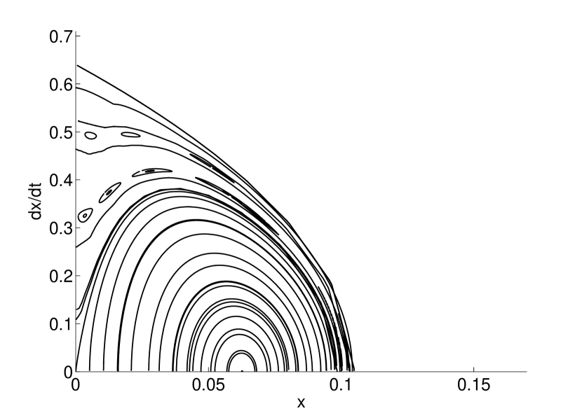
Figure 1a: Surfaces of section for triaxial potential with varying axis weights. (a) Surface of section for nearly spherical version of the potential with $(a,c)$ = $(\sqrt{1.1},\sqrt{0.9})$. (b) Surface of section for moderate axis weights $(a,c)$ = $(1.25,0.75)$, so that the axis ratios are 3:4:5. (c) Surface of section for elongated potential with $(a,c)=(\sqrt{3},\sqrt{2}/2)$. The letters refer to the orbits shown in Figure 2.

Fig. 1 — Continued.

Fig. 1 — Continued.

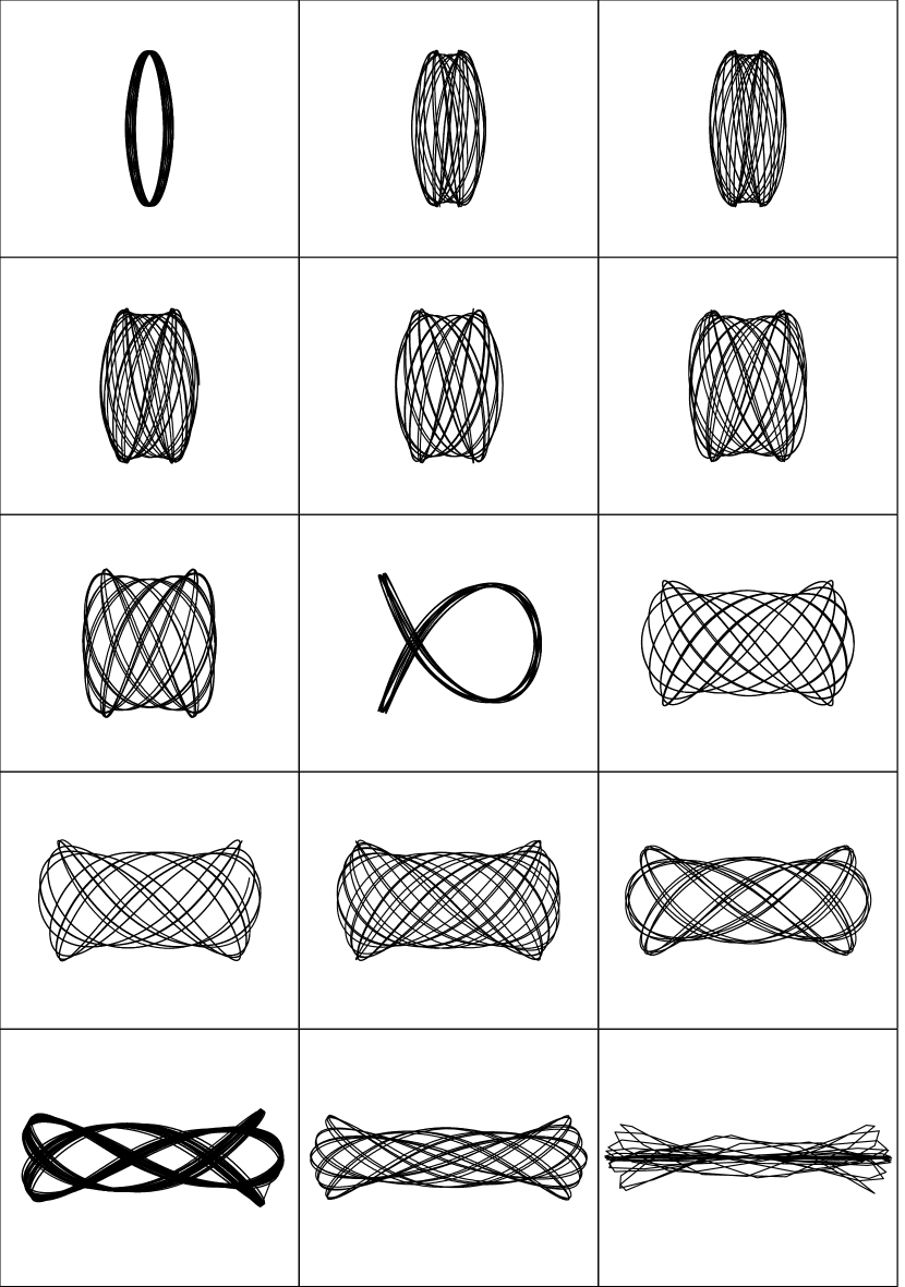
Figure 2: Collection of orbits for triaxial potential with axis parameters $(a,c)=(\sqrt{3},\sqrt{2}/2)$. The panels are labeled by letters ‘a’ – ‘o’, where the labels coincide with those on the surface of section plot shown in Figure 1c.

To illustrate the variety of possible orbits, the third surface of section in Figure 1a includes labels for 15 points in the phase plane (indicated by the letters ‘a’ – ‘o’). Each of these points is associated with a corresponding orbit, which is shown in the 15 panels of Figure 2. Orbit ‘a’ is located in the central region of the phase plane, i.e., the region that dominates for nearly spherical potentials (see Fig. 1a); the corresponding orbit in Figure 2 is thus a tube orbit. The tube orbits become increasingly complicated (see orbits ‘b’ and ‘c’) as one moves out from the central region. The remaining parts of the surface of section primarily correspond to box orbits of varying degrees of complexity. For orbits that lie in the centers of islands in the phase plane, the corresponding orbits show symmetry – for example, orbit ‘i’ is a ‘fish orbit’. Notice that orbits that lie at the centers of islands in the phase plane exhibit this symmetry because they represent “resonant” orbits. For example, the fish orbit in Figure 2 corresponds to a 2:3 resonance in the $x-z$ plane. Note that the orbits in Figure 2 were constructed for purposes of illustration, so that “tighter” fish orbits, closer to exact resonance, can be studied. One should also keep in mind that these orbits are confined to the $x-z$ plane; additional types of orbits can be obtained when the orbit is allowed to explore the full three dimensions of the potential (BT87, PM01). The instability of these orbits to motion in the perpendicular direction is considered in the following section.

Figure 3 shows a typical box orbit in this triaxial potential. The axis ratios are chosen to be moderately triaxial, but not extremely so. This orbits displays a combination of regularity and chaotic behavior. The orbit crosses back and forth across the origin with no well-defined sense of rotation. The crossing time scale is of order unity (in dimensionless units), although it varies slightly from cycle to cycle. The distance of closest approach to the origin also changes from cycle to cycle, but exhibits greater variation. In the discussion of orbital instability that follows, we use this “typical” orbit as a benchmark case to study the instability.

Figure 3: Box orbit initially confined to the $x-z$ plane. The potential is taken to have axes $(a,b,c)=(\sqrt{2},1,0.5071)$. For this orbit, the time average $\langle j\rangle$ of the specific angular momentum approaches zero, so the orbit has no sense of rotation and is thus a box. The orbit crosses near the origin in a quasi-periodic manner, which leads to quasi-periodic forcing of the perturbations in the perpendicular direction (see text).

4 INSTABILITY

A numerical survey of parameter space reveals that many of the orbits that are initially confined to one of the principal planes are unstable to motions in the perpendicular direction. One example of this unstable behavior is shown in Figure 4. In this case, the orbit begins in the $x-z$ plane, but has a small perturbation in the $y$-direction (here $\Delta y=10^{-8}$). As shown in Figure 4, the subsequent evolution of the $y$ coordinate displays four types of behavior: [1] The most striking property of the solution is the overall growth of the amplitude, i.e., the envelope shows exponential growth. [2] The solution exhibits a well-defined periodicity superimposed on the exponential growth. This periodicity is a reflection of the underlying (near) periodicity of the original box orbit in the $x-z$ plane and is thus not unexpected. However, notice that the periodicity has multiple frequencies. [3] The solution displays chaotic irregularities superimposed on the otherwise smooth (regular) function. [4] The growth saturates at a well-defined time scale, and the solution subsequently undergoes long period oscillations (with additional short period oscillations and chaotic irregularities superimposed). In the analysis and discussion given below, our goal is to elucidate the fundamental mechanism(s) responsible for these four properties.

For orbits that begin in a principal plane, the equation of motion in the perpendicular direction (out of plane) determines whether or not the orbit is stable. For a given plane, we can consider the perpendicular coordinate value to be small, at least at the beginning of the evolution. For example, if the original orbit lies in the $y-z$ plane, then the $x$ coordinate is small so that $|x|\ll y,z$. In this limit, the equation of motion for the non-planar direction takes the form

$${d^{2}x\over dt^{2}}+\omega_{x}^{2}x=0\qquad{\rm where}\qquad\omega_{x}^{2}={4/a\over\sqrt{c^{2}y^{2}+b^{2}z^{2}}+a\sqrt{y^{2}+z^{2}}}\ ,$$ (42)

Similarly, for the other two principal planes, the equations of motion for the perpendicular coordinate can be written

$${d^{2}y\over dt^{2}}+\omega_{y}^{2}y=0\qquad{\rm where}\qquad\omega_{y}^{2}={4/b\over\sqrt{c^{2}x^{2}+a^{2}z^{2}}+b\sqrt{x^{2}+z^{2}}}\ ,$$ (43)

and

$${d^{2}z\over dt^{2}}+\omega_{z}^{2}z=0\qquad{\rm where}\qquad\omega_{z}^{2}={4/c\over\sqrt{b^{2}x^{2}+a^{2}y^{2}}+c\sqrt{x^{2}+y^{2}}}\ .$$ (44)

Figure 4: Development of the instability for the box orbit shown in Figure 3. The original orbit lies in the $x-z$ plane with a small perturbation in the perpendicular direction ($\Delta y\sim 10^{-8}$). The amplitude of the perpendicular coordinate (the $\hat{y}$ coordinate) thus starts at $|y|\sim 10^{-8}$ and grows to saturation during $\sim 100$ time units. Note that we take the absolute value of $y(t)$ and that we scale the coordinate by its initial value, so the vertical axis represents the growth factor. Notice also that the time evolution of the perpendicular coordinate simultaneously displays nearly periodic behavior, exponential growth, and chaotic variations; at late times the exponential growth saturates and is replaced by long-period oscillatory behavior.

Figure 5: Driving frequency $\omega^{2}(t)$ as a function of time for the orbit depicted in Figures 3 and 4. This plot represents the effective oscillation frequency of the test particle in the direction perpendicular to the starting plane of the orbit (here, the $\hat{y}$ direction). The three panels show three temporal ranges, i.e., 1000 time units (top), 100 time units (middle), and 10 time units (bottom). Notice that the spikes in $\omega^{2}$ are extremely narrow, much closer to the delta function limit than the cosine limit. Notice also that the forcing function has structure on a wide range of time scales, and shows both periodicity and chaotic behavior.

Figure 6: Histograms showing the distributions of periods (top panel) and forcing strengths (bottom panel) for the orbit considered in Figures 2 – 4. The period is defined to be the time interval between successive maxima in the function $\omega^{2}(t)$ and the forcing strength $q$ is defined to be the peak values of the function (the maxima). Note that the scale for the period, and hence its distribution, is narrow, with mean value $\langle P_{\rm orb}\rangle$ = 0.986, and standard deviation $\sigma_{P}$ = 0.057. In contrast, the distribution of forcing strength is shown using logarithmic binning and spans a wide range, with mean value $\langle q\rangle\approx$ 360 and standard deviation $\sigma_{q}\approx$ 560.

These equations of motion for the perpendicular coordinate (eqs. [42–44]) provide both a qualitative and quantitative explanation for the instability, although the rest of the orbit, described by the other coordinates [e.g., $x(t)$ and $z(t)$], play a role. (In addition, in order to understand the saturation mechansim, we must go beyond the limit of small perpendicular coordinate values — see below.) To fix ideas, we present the driving frequency $\omega_{y}^{2}$ for a box orbit in the $x-z$ plane in Figure 5. This function $\omega^{2}(t)$ is typical for orbits that exhibit instability in the perpendicular coordinate, although the exact form varies with the orbit under consideration. Note that the driving frequency shows both periodic and stochastic behavior. Furthermore, this form for $\omega^{2}$ allows for a qualitative description for the four properties of the unstable solutions listed above:

[1] Instability. At first glance, the equations look like those of a simple harmonic oscillator, which would naively imply stability. Upon closer inspection, however, the functions $\omega^{2}(t)$ are highly time variable and nearly periodic. In the limit where the functions $\omega^{2}(t)$ are exactly periodic, the equations of motion are a type of Hill equation (Hill 1886; Magnus & Winkler 1966, hereafter MW66; Abramowitz & Stegun 1970, hereafter AS70). Since Hill equations are known to have regimes of instability, the fact that we see unstable solutions follows immediately. Notice that in the limit of nearly circular orbits in a nearly spherical potential, the equation of motion for the perpendicular coordinate becomes Mathieu’s equation (§5.3), whose regimes of instability are well studied (AS70, Arfken & Weber 2005, hereafter AW05). This Mathieu-equation limit has been studied previously in a related context (Binney 1981, Scuflaire 1995). Notice also that the driving frequency function $\omega^{2}(t)$ displays extremely narrow spikes, rather than smooth cosine curves, as in Mathieu’s equation, so the latter does not represent a good approximation for most of the parameter space of interest here. We thus consider the opposite limit in which the peaks in the driving frequency function are considered as Dirac delta functions (see §5; Appendices B and C).

[2] Periodicity. The second key feature of the observed unstable solutions is their periodicity. This feature also follows directly from the fact that the perturbation equation is of the Hill variety. In particular, Floquet’s Theorem implies that the Hill equation has solutions of the form

$$y(t)={\rm e}^{i\alpha t}p(t)\,,$$ (45)

where $p(t)$ is a periodic function and where the phase factor can provide a growing (unstable) solution when $\alpha$ is imaginary (MW66, AS70). These previous mathematical results imply that the period of $p(t)$ is either the same as that of the driving frequency $\omega^{2}(t)$ or twice as great. In this context, the periodicity of the driving frequency $\omega^{2}(t)$ is determined by the period of the orbit in the (original) orbit plane. This period, in turn, is given by equations (40) and (41) to a good working approximation. As shown in Figure 5, and indirectly by Figure 3, the driving frequency has multiple periods; this complication leads to the solutions $y(t)$ displaying multiple periodicities as well.

[3] Chaos. The motion of the perpendicular coordinate is ultimately driven by the (time dependent) coordinates of the starting orbit (in its initial plane). The amplitude of the driving frequency oscillations $\omega^{2}(t)$ is essentially determined by the distance of closest approach of the orbit to the origin (see eqs. [42 – 44]) and this distance varies from passage to passage. If the orbit is chaotic, as is often the case, these distances of closest approaches will be given by some distribution of values, and the corresponding driving frequency will have a chaotic element.

One might worry that departures from exact periodicity would invalidate previous mathematical results concerning instability. This issue led us to analyze the quasi-periodic Hill’s equation with random forcing strengths (Adams & Bloch 2007, hereafter AB07). These new results show that the departures from strict periodicity in Hill’s equation result in a re-scaling of the parameters, but do not otherwise compromise the instability (see Theorem 1 of AB07; see also Appendix D). In addition, the stochastic variations in the forcing function lead to two separate contributions to the growth rate: an asymptotic growth rate that results from a direct application of Floquet’s theorem, and an anomalous growth rate that results from matching the solutions from cycle to cycle, where each cycle has a different forcing strength (see Theorem 2 of AB07).

The distributions of periods and forcing strengths thus play an important role in determining the dynamics. For the box orbit depicted in Figure 3, and the corresponding forcing function $\omega^{2}(t)$ shown in Figure 5, we show the distributions of periods and forcing strengths in Figure 6. For the sake of definiteness, we have defined the period to be the time interval between peaks of the function $\omega^{2}(t)$. The forcing strengths ($q$) are defined to be the heights of the peaks. Although the distributions of period and forcing strength vary with the orbit under consideration, Figure 6 reveals several important and typical trends: The distribution of periods is quite narrow, so that departures from strict periodicity are small. This finding makes the corrections for varying periods corrrespondingly small (where this statement is quantified in Appendix D). On the other hand, the distribution of forcing strengths $q$ is wide, with the standard deviation larger than the mean. Both the mean value (appropriately weighted) and the width of the distribution play a role in determining the growth rates for instability.

In addition to chaotic behavior within a given orbit, the variation of dynamical properties varies from orbit to orbit, even those with almost the same starting conditions. The orbits thus display sensitive dependence on their initial conditions, one of the defining properties of chaotic systems. As one example of this behavior, Figure 7 shows the growth rate of the instability plotted as a function of the starting $x$-coordinate. This plot shows that nearby starting trajectories can result in significantly different growth rates. Since the growth of the $y$-coordinate is not perfectly exponential, some ambiguity arises in the definition of the growth rate. The results shown in Figure 7 were obtained by finding the maximum value $|y|_{max}$ of the $y$-coordinate over the first 50 time units, and defining $\gamma\equiv\ln|y_{max}|/50$; these growth rates thus represent the average growth rates over this time interval. Figure 7 also shows the saturation level of the perpendicular coordinate (in the lower panel) plotted as a function of the same starting conditions. Here, the saturation levels were computed by finding the maximum displacement over the first 200 time units (thereby allowing the instability time to saturate). The behavior of the saturation level is also highly structured, i.e., not a smooth function of $x_{0}/x_{max}$. The fine scale structures in both the growth rate and the saturation level (when considered as a function of $x_{0}/x_{max}$) arise (in part) from the narrow bands of stability that are always present in the Hill’s equation that describes the instability (see AS70, Weinstein & Keller 1987, AB07, and §5 below). Further, we find that the saturation levels correlate with the growth rates; in particular, low or vanishing growth rates correspond to low saturation levels, as expected. Figure 7 shows additional systematic behavior, in that the ranges of starting conditions that lead to large growth rates and large saturation levels are relatively well-defined. The larger structures in the growth rate functions (and saturation levels) often coincide with the structure of the phase-plane diagram for this potential.

Figure 7: The upper panel shows the growth rate of instability as a function of starting coordinate. For all of the cases considered here, the energy is taken to be $E$ = 0.1, and the axis variables $b$ = 1 and $c=\sqrt{2}/2$. Solid curve shows the growth rate $\gamma$ for varying starting locations for the axis parameter $a$ = $\sqrt{3/2}$; the dashed and dotted curves show the results for $a$ = $\sqrt{3}$ and $a$ = $\sqrt{6}$, respectively. The bottom panel shows the corresponding saturation level, i.e., the maximum value of the $y$ coordinate expressed as a fraction of the typical $x$ coordinate. The three curves correspond to the three values of $a$ in the top panel.

[4] Saturation. The strength of the instability, as well as its existence, depends on the amplitude of the driving frequency $\omega^{2}(t)$. The equations of motion found above are derived in the limit where the perpendicular coordinate is small compared to the coordinates in the (initial) orbit plane. As the perpendicular coordinate grows, this approximation becomes invalid, and the relevant equation of motion takes on a modified form. For the cases of interest here, the driving frequencies have the basic form $\omega^{2}(t)\sim 1/{{\hat{\xi}}}$, where ${{\hat{\xi}}}$ is a modified “radial coordinate” where the $(x,y,z)$ coordinates are weighted differently, by the geometric factors ($a,b,c$). As the perpendicular coordinate (e.g,. $y$) grows, its contribution to ${{\hat{\xi}}}$ and hence the driving function becomes significant, with the net effect being to reduce the forcing amplitude. When the amplitude decreases enough, the motion is no longer unstable in the perpendicular coordinate, and the instability saturates.

As a particular example of the behavior described above, we consider the equation of motion for the $\hat{y}$ coordinate for an orbit initially confined to the $x-z$ plane in the limit of a nearly spherical potential (eq. [27]), i.e.,

$${d^{2}y\over dt^{2}}+{1\over 2\xi}\Bigl{[}1+{\delta(x^{2}-z^{2})\over 4\xi^{2}}\,\Bigr{]}y=0\,.$$ (46)

When the $y$ coordinate is small (compared to $x$ and $z$), the size of the driving term is determined by $1/\xi\sim(x^{2}+z^{2})^{-1/2}$. The forcing term is large for small values of displacement $\xi$. When the $y$ coordinate grows, however, its contribution to $\xi$ becomes significant (i.e., $\xi$ is not necessarily small even when $|x|,|z|\ll 1$), and the instability saturates.

To see this trend explicitly, let $\xi=(d^{2}+t^{4})^{1/2}$, where this form assumes that the orbit has a distance of closest approach $d$ and the radius of the orbit is given by a constant force law (appropriate for radial orbits – see §3.2). For a nearly linear orbit with closest approach $d$, the radial distance is given by $\xi^{2}=d^{2}+s^{2}$, where $s$ is the distance along the orbit measured from the point of closest approach. Since $s\propto t^{2}$ for a constant force law, one obtains the relation $\xi^{2}=d^{2}+t^{4}$ in appropriate dimensionless units. The effective amplitude of the driving frequency is then given by the integral

$$q=\int_{-\infty}^{\infty}{dt\over(d^{2}+t^{4})^{1/2}}={8\,\Gamma^{2}(5/4)\over\sqrt{\pi d\,}}\approx{3.71\over\sqrt{d\,}}\,.$$ (47)

At the start of the evolution, when the motion is confined to a plane, the distance of closest approach to the origin $d=d_{0}$ is given by that of the starting orbit. For a box orbit, $d_{0}$ can be quite small, so that $q$ is large. A general property of Hill’s equations is that larger $q$ implies greater instability (although islands of stability will remain – see MW66, AS70, and §5 below). Once the instability has developed, the distance of closet approach must include the displacement in the perpendicular direction, so that $d\to{\langle y\rangle}$ (where the angular brackets represent an appropriate average of the perpendicular coordinate). The value of $q$ at later times is thus reduced by a factor $(d_{0}/{\langle y\rangle})^{1/2}$. Notice that saturation of the instability requires that ${\langle y\rangle}\gg d_{0}$, which is much less restrictive than the requirement ${\langle y\rangle}\sim d_{max}$. In other words, the instability can saturate when the perpendicular displacement, measured here by ${\langle y\rangle}$, becomes sufficiently larger than the (initial) distance of closest approach, but need not be comparable to the full orbit size. In many cases, however, the saturation levels are large enough that ${\langle y\rangle}$ is comparable to the original orbital extent in the $x-z$ plane (see Fig. 7).

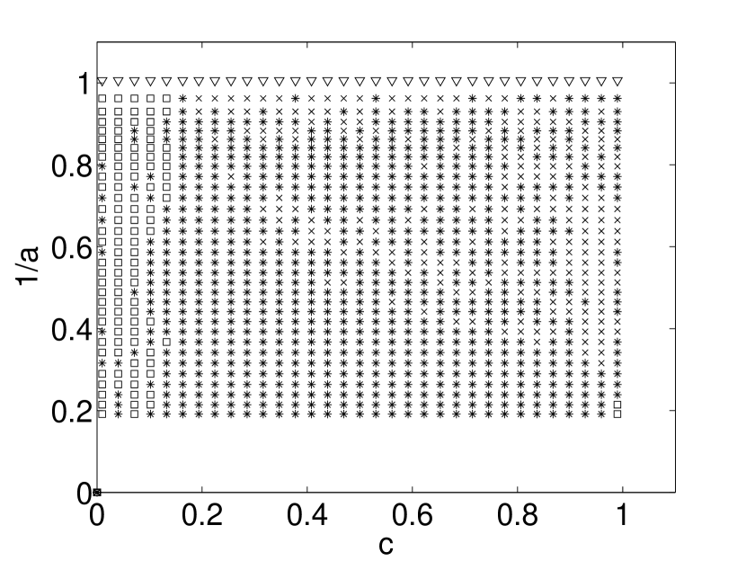
Figure 8a: Instability as a function of axis weights. Nearly spherical potentials correspond to the upper right corner of each panel. For each point in the grid, orbits are started in the $x-z$ plane, with fixed energy, and with a fixed starting value of the $\hat{x}$ coordinate. The symbols denote the type of resulting orbits, where open squares are stable box orbits, open triangles are stable loop orbits, stars are unstable box orbits, and crosses are unstable loop orbits. (a) Result for $x_{0}/x_{max}$ = 0.10. (b) Result for $x_{0}/x_{max}$ = 0.50. (c) Result for $x_{0}/x_{max}$ = 0.90.

Fig. 8 — Continued.

Fig. 8 — Continued.

Before leaving this section we consider the degree of stability versus instability as a function of the shape of the triaxial potential, where shape is codified by the axis weights $(a,b,c)$. For a given energy and set of axis weights, we start orbits with a given value of $x_{0}/x_{max}$ as described in §3. We then determine if the orbit is a loop orbit or a box orbit, and whether the orbit is stable or not. To determine the orbit class, we use a procedure similar to that developed by Fulton & Barnes (2001). For a given orbit, we fourier analyze both time series $x(t)$ and $z(t)$ and obtain the dominant frequencies. If the dominant frequencies are in 1-1 correspondence, the orbit is labeled as a loop (where we allow for a 5% discrepancy in the frequency ratio). To determine if the orbit is unstable, we monitor the maximum displacement $|y|_{M}$ in the perpendicular direction. If the perpendicular coordinate grows above a given threshold, then the orbit is considered unstable. Since orbits generally either grow and saturate at large values of $|y|_{M}$, or remain stable with small values of $y\sim 10^{-8}$, the results are insensitive to the threshold value. For the sake of definiteness we use a threshold $|y|_{M}/r_{M}\geq 0.01$ (where $r_{M}$ is the maximum two-dimensional radius in the original $x-z$ plane of the orbit). The results are shown in Figure 8a for three different values of the starting $\hat{x}$ coordinate. Several trends are evident. In all cases, a significant fraction of the plane shows unstable orbits, so that the instability considered herein is indeed robust. As the starting value $x_{0}/x_{max}$ is increased, the orbits become more nearly “radial” (following the $\hat{x}$ axis) and the degree of instability decreases somewhat (compare the panels of Fig. 8a); further, the regimes of stability (usually) correspond to extreme axis weights (small $c$ and large $a$). Finally, we note that the regimes of stability and instability are intermixed, as expected in highly chaotic systems.

5 MODEL EQUATIONS

In this section we develop and analyze a class of model equations that captures the essential physics of the orbit instability found above. As shown in the previous section, when the motion is initially confined to one of the principal planes, the equation of motion for the amplitude of the perpendicular coordinate takes the form

$${d^{2}y\over dt^{2}}+[{\lambda}+Q(t)]y=0\,,$$ (48)

where $Q(t)$ is nearly periodic. Here we use the variable $y$ as the perpendicular coordinate, but the same general form holds for the perturbation direction falling along any of the axes. Note that we have separated out part of the forcing function as a baseline frequency $\sqrt{{\lambda}}$, although this decomposition is not unique. Notice also that the function $Q(t)$ can be considered as a function of the form $Q[x(t),z(t)]$, where $x(t)$ and $z(t)$ describe the orbital motion in the original plane, so that $Q$ is given by equations (18–20) in general and by equations (42–44) in the limit of small $y$ (as assumed here).

In most applications, $Q(t)$ will be nearly periodic because its time variation is given by an orbit solution, although the crossing time of the orbit can vary from cycle to cycle. In this context, in the Hernquist potential, the orbital periods depend on energy, but are nearly independent of angular momentum (see Fig. 3 of AB05), especially in the inner limit as considered here, so that the cyclic forcings have nearly the same time intervals. This expectation is borne out in numerical evaluations of the orbits, as shown in the distributions of Figure 6. On the other hand, the amplitude (the forcing strength) varies substantially from cycle to cycle. If the function $Q(t)$ is exactly periodic, then the relevant equation of motion has the form of Hill’s equation (Hill 1886), and we can draw on a number of well-known results (MW66, AS70, Arnold 1978). In this section we consider the periodic version of Hill’s equation as a first approximation, and then show how to generalize the results to cases where the forcing strength varies from cycle to cycle. This section is augmented by Appendices B – D, which include some of the mathematical details, and by Appendix E, which presents a heuristic review of Hill’s equation. We consider a more rigorous mathematical treatment of the stochastic problem in a separate publication (AB07).

5.1 The Delta Function Limit

As a first approximation, we consider the forcing potential to be sufficiently sharp that we can model $Q(t)$ with a Dirac delta function. In physical terms, this approximation means that the orbit passes close to the origin (so that the spike in $Q(t)$ is large) and that the orbit spends little time near the origin (so the spike is narrow). Both of these conditions are met for box orbits in triaxial potentials. In this limit, the equation of motion for the perpendicular coordinate takes the particular form

$${d^{2}y\over dt^{2}}+[{\lambda}+q\delta({[t]}-\pi/2)]y=0\,,$$ (49)

where $q$ measures the strength of the spike and where $\delta$ is the Dirac delta function. Here we have scaled the time variable so the period of one cycle is $\pi$. Note that the argument of the delta function is written in terms of ${[t]}$, which corresponds to the time variable mod-$\pi$, so that the forcing potential is $\pi$-periodic. Notice also that the actual physical problem has a forcing strength $q$ that varies from cycle to cycle. As a result, we should think of the “constant” $q$ as a stochastic variable that takes on a new value every cycle $0\leq{[t]}\leq\pi$.

In the delta function limit, the solution to Hill’s equation is thus specified by two parameters: the frequency parameter $\lambda$ and the forcing strength $q$. The solutions to equation (49) are constructed in Appendix B along with the determination of the growth rates for instability. Figure 9 shows the plane of possible parameter space for Hill’s equation in this limit, with the unstable regions shaded. Notice that a large fraction of the plane is unstable. This result is in keeping with our previous finding that the equation of motion for the instability takes the form of a Hill’s equation with highly spiked forcing functions and that a large fraction of the orbits are unstable (§4).

An important feature of these solutions is that in the limit of large forcing strength $q\gg 1$, the bands of stability become extremely narrow — but they never vanish entirely. Physical orbits are often found in this limit, as illustrated by Figures 5 and 6. This property is generic to Hill’s equations in the unstable (here, large $q$) limit (Weinstein & Keller 1987). For the case of delta function forcing terms, for example, the widths of the stable zones are given by $(\Delta\lambda)=(8n^{2}/\pi)\langle 1/q\rangle$, where $n$ labels the order of the stability strip (AB07). The presence of these narrow zones implies that the issue of stability/instability can depend sensitively on the orbit parameters, i.e., nearby orbits can display significantly different behavior. This trend is seen in the numerical results for the growth rates, as depicted in Figure 7, where the function $\gamma(x_{0}/x_{\rm max})$ displays a great deal of structure, so that orbits with nearly identical starting conditions can have significantly different growth rates.

With the solution to the model equation in hand, as illustrated by Figure 9, it is useful to reconnect with the original orbit problem. In terms of physical orbits, the period of the (periodic) forcing potential is determined by the crossing time $t_{cross}$ of the orbit. Here we have defined the dimensionless time variable $t$ so that the period is $\pi$; the physical time variable $t_{phys}$ is thus related to the dimensionless time appearing in equation (49) via $t_{phys}=t(t_{cross}/\pi)$. Further, the period of a half orbit for the spherical limit is given (almost) analytically in AB05,

$$\tau_{1/2}=(4\pi G\rho_{0})^{-1/2}\epsilon^{-3/2}\left\{\cos\sqrt{\epsilon}+\sqrt{\epsilon}\sqrt{1-\epsilon}\right\}{\cal A}\,,$$ (50)

where $\epsilon=|E/\Psi_{0}|$ is the dimensionless energy and where the correction factor $\cal A$ lies in the range $1\leq{\cal A}\leq 1.05$ (see Fig. 3 of AB05). The strength $q$ of the forcing potential is determined by the distance of closest approach of the orbit to the origin ($q\sim 1/d$). In the spherical limit, the distance of closest approach is given by the inner turning point of the orbit and is a simple function of energy and angular momentum (AB05). Here, for loop orbits, the orbit has an analogous inner turning point and the spherical results can be used as a good starting approximation. For box orbits, the test particle wanders arbitrarily close to the origin, so that the distance of closest approach will often be small (and hence the parameter $q$ will be large); in general, $q$ can vary from cycle to cycle. The problem of Hill’s equation with random variations in forcing strength is addressed in Appendix C for the delta function limit (see AB07 for a more general treatment).

Figure 9: Regions of instability for Hill’s equation in the delta function limit. The shaded regions show the values of $(\lambda,q)$ that correspond to exponentially growing (unstable) solutions, which represent unstable growth of the perpendicular coordinate for orbits in our triaxial potential that are initially confined to one of the principal planes (see also AB07).

5.2 Beyond the Delta Function Approximation

The physical orbits do not produce perfect delta functions for the forcing potential $Q(t)$. Instead, the spikes have a small but finite width. In order to understand how this feature affects the growth rates (in particular, the regions of stability and instability), we model the forcing function through an equation of the form

$${d^{2}\xi\over dt^{2}}+\bigl{[}{\lambda}+q_{n}\sin^{n}t\bigr{]}\xi=0\,,$$ (51)

where $n$ is a (generally large) even integer. For the class of orbits considered in the previous section, we have fit functions of the form $\sin^{n}t$ to the functions $\omega^{2}(t)$ resulting from numerical integration of the equations of motion. The values of $n$ required to fit these results fall in the range $n=10-100$, with a “typical” best-fit value $n\approx 64$. The full width at half maximum (FWHM) of the spike is given by $w\approx 2([2\ln 2]/n)^{1/2}$ in the limit of large $n$ where the spikes have narrow widths. For $n$ = 64, for example, we obtain $w\approx 0.294$.

To compare model equations of this form for different values of $n$, or to compare with the delta function limit, one needs to define the effective forcing strength for a given value of $q_{n}$. In the delta function limit, this term has the form $q\delta([t]-\pi/2)$. Since the delta function integrates to unity over one cycle, we can define the effective strength $q_{\rm eff}$ for a given $n$ through the relation

$$q_{\rm eff}=q_{n}\int_{0}^{\pi}\sin^{n}dt=q_{n}\pi{(n-1)!!\over n!!}\,.$$ (52)

Figure 10 shows the plane of parameters $(\lambda,q_{eff})$ for a Hill’s equation of the form given by equation (51) with $n$ = 64. The $q$ values have been scaled according to the normalization of equation (52) so that this plane can be directly compared with Figure 9. After including this normalization, the two planes are more similar than different, so that we expect the delta function model of the previous subsection to provide a good description of the instability mechanism. Nonetheless, Figures 9 and 10 show slight differences, with the “tongues of instability” being somewhat narrower for the case with $\omega^{2}$ spikes of finite width.

Figure 10: Regions of instability for Hill’s equation for periodic spikes with nonzero width. The width is given by $\sin^{n}t$ where $n$ = 64. The shaded regions show the values of $(\lambda,q_{eff})$ that correspond to exponentially growing (unstable) solutions (compare with Fig. 9). Note that the values of $q_{eff}$ have been normalized according to equation (52).

5.3 The Nearly Spherical (Mathieu Equation) Limit

We note that previous treatments of similar orbit instabilities (e.g., Binney 1981, Scuflaire 1995) often find that the equation of motion for the perpendicular coordinate (whose motion can be unstable) takes the form of Mathieu’s equation

$${d^{2}y\over dt^{2}}+(a+q\cos t)y=0\,.$$ (53)

Although this equation has qualitatively similar instabilities to those considered here (compare the results presented in AS70 with Figures 9 and 10; see also Binney 1981), the forcing function $\omega^{2}\sim\cos t$ is extremely different from that shown in Figure 5. It is thus useful to find the limiting regime of parameter space for which the instability takes the form of Mathieu’s equation, rather than the more extreme, nearly delta function limit considered above.

In qualitative terms, in the limit of a nearly spherical system (§2.5), the equation of motion for the perturbation takes the simpler form

$${d^{2}y\over dt^{2}}+{2\over\xi}y=0\,,$$ (54)

where $\xi^{2}=x^{2}+y^{2}+z^{2}$ and where we have assumed motion initially confined to the $x-z$ plane. If we also consider the initial orbit to be nearly circular, then we can define an effective radial coordinate of the orbit $r^{2}=x^{2}+z^{2}$. The forcing term thus takes the form

$$\omega^{2}={2\over\xi}\approx{1\over r(t)}\approx{1\over r_{0}+(\Delta r)\cos\Omega t}\,,$$ (55)

where $r_{0}$ plays the role of the semimajor axis of the orbit, the turning points of the orbit fall at $r_{0}\pm\Delta r$, and $\Omega$ is the mean motion of the orbit (since the orbit is not an ellipse, these quantities have slightly different meaning than in the standard Kepler problem – see AB05 for further discussion). With one further approximation, assuming $\Delta r\ll r_{0}$, the equation of motion for the instability takes the form

$${d^{2}y\over dt^{2}}+{2\over r_{0}}\Bigl{[}1-{\Delta r\over r_{0}}\cos\Omega t\Bigr{]}y=0\,,$$ (56)

which has the form of Mathieu’s equation. Although this result was derived for a nearly spherical potential, the loop orbits in triaxial potentials also result in Mathieu-like equations for the instability of the perpendicular coordinate (although the fraction of loop orbits tends to decrease with increasing levels of triaxiality). Note that Mathieu’s equation can also be transformed into a discrete map using the same procedure as described in the previous subsections.

6 CONCLUSION

6.1 Summary of Dynamical Results

Analytic results: One set of results from this paper is the development of a collection of analytic expressions that describe potentials, forces, and orbits for the triaxial generalization of the Hernquist/NFW profile in the inner limit. In particular, we have found a completely analytic form for the potential (eqs. [10 – 17]), the force terms (eqs. [18 – 20]; see also PM01), the axis ratios of the potential (eqs. [21 – 24]), and the potential in the limit of nearly spherical density profiles (eqs. [27 – 28]). We have also found the radial solutions in the spherical limit for the full Hernquist potential (§3.3), i.e., valid over all radii $0<\xi<\infty$, not just the inner limit $\xi\ll 1$. Finally, for the axisymmetric version of the NFW profile, we have found analytic expressions for the potential and the force terms that are valid over the entire radial range of the halo (see Appendix A).

Another contribution of this paper is an analytic formulation of the instability problem. For orbits initially confined to one of the principal planes, the equation of motion for the perpendicular component takes a relatively simple form (eqs. [42 – 44]). Further, the instability can be described in terms of simple model equations (§5, Appendices B – D) that allow for an analytic description of the instability. Since these equations of motion have the form of Hill’s equation, we can utilize a large collection of known results (AS70, AW05, MW66). In this context, however, the relevant Hill’s equations have random forcing terms (forcing strengths that vary from cycle to cycle), which requires the development of new mathematical results. We have addressed this complication in a separate companion paper (AB07).

In addition to their usefulness in providing physical understanding of orbits and their instabilities, these analytic results are also useful for computational purposes. Although all of these results can also be determined numerically, the regime of parameter space is enormous, so that analytic results provide a substantial savings in the required computational effort. Analytic results also aid in our understanding of the underlying mechanism for the instability, as outlined below.

Overview of the instability: The main focus of this paper is to demonstrate that for orbits initially confined to any of the principal planes, the motion in the perpendicular direction is unstable to growth; our related objective is to understand the underlying mechanism for the instability. As discussed in §4, the instability displays four key features: quasi-periodic oscillatory behavior, exponential growth, superimposed chaotic variations, and eventual saturation. These four features can be understood as follows:

For a given energy, an orbit has a well-defined crossing time, which naturally gives rise to quasi-periodic behavior. Furthermore, this property provides an effective periodic forcing potential for the motion in the direction perpendicular to the original orbital plane. The resulting dynamics can thus be described with a Mathieu-Hill-like equation, which is well-known to have unstable (growing) solutions (MW66, AS70, AW05). As a result, for a wide range of parameters, the motion in the perpendicular direction will be unstable. In the case of a “pure” Hill’s equation, with precisely periodic forcing, the growing solutions have exponential growth superimposed on periodic oscillations, as seen in the instability under study. The period of the growing solutions is given by the period of the forcing function, which is determined here by the crossing time of the orbit in the original plane. Thus, the first two properties of the instability (periodic behavior and exponential growth) follow directly from the form of the equation of motion for the perpendicular coordinate (eqs. [42 – 44]).

Chaotic variations represent the next property of the instability and they arise due to the triaxial nature of the potential (which arises from the triaxial density profile). As is well known (BT87), triaxial potentials allow for box orbits, and for chaotic behavior, and both of these effects are increasingly common as the axis ratios of the triaxial potential become more extreme. For sufficiently triaxial potentials, the crossing time varies from cycle to cycle and hence the frequency of the forcing of the instability varies somewhat. However, a much more significant effect is that the strength of the forcing varies from cycle to cycle. In this case, the forcing strength is determined by the distance of closest approach of the orbit to the origin in the original plane, where this distance is weighted by the axis weights $(a,b,c)$ of the triaxial potential. For example, box orbits are quasi-periodic and wander arbitrarily close to the origin. Thus, as the orbit varies chaotically in its original plane, the forcing terms for the instability vary as well, and these chaotic variations appear in the growing (unstable) solution for the perpendicular coordinate.

The final property of the unstable solutions is their eventual saturation. This behavior is expected for two reasons: In physical terms, the full three dimensional orbit must conserve energy, so there is a limit to the amplitude of oscillations in the perpendicular (unstable) direction, i.e., saturation is inevitable. In mathematical terms, the forcing strength depends (inversely) on the distance of closet approach to the origin; for orbits with sufficiently large values of the perpendicular coordinate, the forcing strength becomes small and the instability stalls.

Model equations: We have analyzed the instability of Hill’s equation in the delta function limit, where the forcing terms are localized in time. In this limit, the equation of motion can be solved analytically for a given cycle of the motion in the original plane. As a result, the growth rates for a pure Hill’s equation can also be found analytically (§5 and Appendix B). For the case of forcing strengths that vary from cycle to cycle, we have found estimates for the growth rates in terms of the expectation value of the growth rates for individual cycles (Appendix C). In the limit of highly unstable systems, this expectation value – the asymptotic growth rate – provides a good working estimate. However, the true growth rate contains an additional component (the anomalous growth rate) that arises from the matching conditions at the cycle boundaries. In a separate paper we show that this correction term can be found analytically in terms of an expectation value (see AB07), and we present general theorems regarding the instability and growth rates for Hill’s equation with random forcing terms.

The $\hat{y}$ direction is most unstable: Although orbits around all three axes are unstable, the orbits around the intermediate ($\hat{y}$) axis are more likely to be unstable: The instability we are exploring here is often strongest when the motion in the original plane arises from box orbits, which are more likely to take place when the axis ratios of the two axes in the original orbit plane are more extreme (BT87). The “$\hat{y}$ instability” takes place when the original orbit lies in the $x-z$ plane, and the axis ratio $a/c$ is the largest by definition. Therefore, the $\hat{y}$ instability is the most likely to occur; alternatively, the growth rate for the $\hat{y}$ instability is likely to be larger than that for the other two cases. One should compare with situation with the classic result from rigid-body dynamics: As is well-known, rotation about the shortest or longest axis of an asymmetric rigid body produces stable motion, whereas rotation about the intermediate axis is unstable.

6.2 Astrophysical Implications

Although this paper focuses on the description of the triaxial potential, its orbits, and the corresponding orbital instabilities, these results can be applied to a number of astrophysical systems on a variety of size scales. On the largest scales, this work applies to the inner regions of dark matter halos – both for galaxies and galaxy clusters. On smaller scales, these results are applicable to the dynamics of tidal streams, galactic bulges and warps, and young embedded star clusters. All of these systems (or the inner portions of them) are described by the triaxial potential developed herein, and can be potentially affected by this orbit instability. These applications are briefly outlined below, but we emphasize that they should be explored in greater depth.

For completeness, we note that in real astrophysical systems, the gravitational potential will never be completely smooth as assumed here. Instead, stars and other inhomogeneities provide a nonzero level of graininess to the potential, and will thereby contribute to the degree of chaos in the constituent orbits. In terms of the instability considered here, these irregularities guarantee that orbits cannot be exactly confined to any given plane; instead, these effects act to set the smallest possible amplitude for perturbations in the direction perpendicular to the starting plane. We also note that the instability considered here strictly applies only to orbits that start in one of the principal planes, and such orbits represent only a small portion of phase space.

Dark Matter Halos: In dark matter halos, both the orbits of dark matter particles themselves and the orbits of sub-halos benefit from an analytic description, which can aid in understanding how dark matter halos achieve the (nearly) universal form observed in numerical simulations (starting with NFW). Another finding from numerical simulations is that the velocity distributions are generally radial in the outer parts of the halo and more isotropic in the inner regions. This isotropization cannot take place through two-body relaxation processes, as the time scale is much too long. The orbit instability considered in this paper can provide at least a partial explanation: The inner regions tend to have triaxial forms with density profiles $\rho\sim 1/m$ in the inner limit, i.e., the form of the density and potential considered in this paper. Since nearly radial orbits are subject to the orbit instability considered herein, the inner halo cannot maintain purely radial velocity distributions. Further, both the time scale (several crossing times) and the saturation level (the amplitudes of the perpendicular coordinate oscillations become roughly comparable to those in the original orbit plane) suggest that the velocity distribution can become sufficiently isotropic to explain the results of numerical simulations. The velocity distributions of dark matter particles, as well as their enhancements in tidal streams (see below), can affect direct detection strategies (e.g., Evans et al. 2000).

Tidal Streams: Since tidal streams must orbit in galactic potentials with some triaxial aspect, the results of this paper also inform their dynamical properties. The coherence of tidal streams relies on the orbits of the satellite galaxies and the stars that are stripped away from them to remain coherent for a number of orbits. In contrast, the instability studied in this paper can act to disrupt tidal streams. This disruption could have important implications for direct searches for dark matter, through particle detection experiments, where enhancement due to tidal streams has been invoked as a way to help discriminate the signal from the background (Evans et al. 2000). Turning the problem around, one can also use the observed properties of tidal streams as a means to constrain the triaxiality of their galactic potentials (Ibata et al. 2001). This instability will also play a role in the assimilation of merging substructures during the galaxy formation process (e.g., Helmi et al. 1999). In all of these applications, however, the number of orbits of the satellites is relatively small (several), and it could be hard to distinguish between precession of an ordinary orbit in a triaxial potential and this instability. Further exploration of this issues is necessary.

Galactic Bulges and Disks: The orbits and instabilities studied in this paper can also act on the scale of galactic bulges, which can be described by a triaxial generalization of the Hernquist potential. In this context, an important issue is how often stars wander close to the potential center, where (usually) a supermassive black hole resides. The orbit instability studied herein acts to change nearly radial orbits into orbits with more isotropic velocity ellipsoids, and thereby changes the rate at which stars interact with the central black hole. We note that near the galactic center, the gravitational potential of the black hole itself must be taken into account. Some work along these lines has been done (Gerhard & Binney 1985; PM01, Poon & Merritt 2002), which shows that triaxiality leads to more box orbits and greater rates of stellar accretion by a central black hole; on the other hand, the orbit instability studied herein acts to increase the distance of closest approach and thereby suppresses accretion of stars. In any case, this issue provides an interesting problem for future study.

A related issue is that sufficiently distorted (non-axisymmetric) disk galaxies can be subject to this type of orbit instability, which acts to populate regions out of the original disk plane. This issue was explored earlier by Binney (1981) using the triaxial version of the logarithmic potential; this work can be used to extend such previous analyses by providing a different potential and considering forcing frequencies $\omega^{2}(t)$ that have stochastic amplitude variations from cycle to cycle and are highly nonlinear (e.g., closer to the delta function limit than the cosine forcing functions that arise for nearly spherical potentials – see §5.3). Both gas and stars can be subject to this instability in galactic disks, leading to galactic warps and other interesting structure (e.g., Sparke 1995, 2002).

Embedded Star Clusters: The dynamics of young embedded star clusters can also be described using the inner limit of the Hernquist potential (Larson 1985, Jijina et al. 1999, Adams et al. 2006). These clusters are expected to have more extreme axis ratios than the larger scale systems considered above. Observations of embedded clusters (Lada & Lada 2003 and references therein) show that the youngest systems are highly irregular, displaying large departures from spherical symmetry. Somewhat older systems (a few Myr) are significantly more spherical, so that the process of isotropization takes place rapidly. In these systems, orbits can be altered through star-star scattering events (where the stars generally have accompanying disks and/or planets) and through the instability studied in this paper. If these young clusters form out of initial gas configurations that are highly flattened, this instability will act to populate the regions perpendicular to the initial cloud plane. The resulting stellar clusters can thereby become more nearly spherical, even in the absence of stellar scattering interactions. For example, suppose that the initial cluster is flattened with a 10:1 aspect ratio ($c$ = 0.1). For the orbit instability of this paper to round out the cluster, the growth rate $\gamma$ must be large enough to compete with stellar scattering. The number $N_{C}$ of crossing times required for the instability to amplify the motion in the perpendicular direction is given by $N_{C}\approx(\ln 10)/\gamma t_{c}$. For a purely stellar system, the ratio of the dynamical relaxation time to the crossing time (BT87) is given by $N_{C}\approx{N_{\star}}/(10\ln{N_{\star}})$; for an embedded cluster dominated by its gas content, however, the relaxation time is longer so that $N_{C}\approx({N_{\star}}/\epsilon^{2})/[10\ln({N_{\star}}/\epsilon)]$, where $\epsilon$ is the star formation efficiency within the cluster (Adams & Myers 2001). These relations imply that orbit instability competes with dynamical relaxation when $\gamma t_{c}>10\epsilon^{2}\ln 10\ln({N_{\star}}/\epsilon)/{N_{\star}}$. For typical values (${N_{\star}}$ = 300 and $\epsilon$ = 1/3), this constraint becomes $\gamma t_{c}>0.058$, a condition is that is often met. As a result, orbit instabilities can dominate stellar scattering as a means to isotropize young embedded star clusters. In addition, the triaxial nature of the potential in these clusters allows young star/disk systems to execute box orbits, which bring the disks closer to the massive stars at the cluster center. Triaxial potentials thus allow for greater radiation exposure for star/disk systems, compared with spherical clusters, or at least a wider distribution of radiative flux experienced by individual solar systems.

6.3 Discussion and Future Work

In addition to the applications outlined above, another issue is to consider how this orbit instability affects the construction of self-consistent galaxy models. In systems where the orbiting bodies provide the source of the potential (e.g., stars in a galactic setting) one must find self-consistent models where the orbiting stars provide the gravity for the triaxial potential (Schwarzschild 1979). This issue is of particular importance for the intermediate scale of galaxies and galactic bulges, and can be complicated by the presence of supermassive black holes (e.g., Poon & Merritt 2002). On the larger scale of dark matter halos, the dark matter particles provide the source (mass) for the gravitational potential. For these systems, however, N-body simulations of large scale structure already self-consistently take into account the orbits of the particles (subject to finite numerical resolution) and are the motivation for both the particular forms for the density profiles (NFW, Hernquist) and their degree of triaxiality. Finally, on the smaller size scale of embedded stellar clusters, the gravitational potential is dominated by gas, which is subjected to additional forces (e.g., magnetic fields) and does not execute the same orbits. As a result, in these systems the background potential can be taken as fixed, at least for purposes of studying this orbit instability.

The analysis of this paper is limited to the case of density profiles that have the form $\rho\sim 1/r$ in the spherical limit, and this form is applicable to only the inner regions of the extended mass distributions in question. Future work should consider both the generalization to other inner limiting forms (e.g., power-law density profiles with other indices, $\rho\sim 1/m^{\gamma}$) and extension of the potential out to all radii. Toward this latter goal, we present the potential and force terms for the axisymmetric version of the NFW profile in Appendix A. In addition to the study of other density profiles, the available parameter space for the potentials considered in this paper is enormous, and should be explored in greater depth. For example, the case of resonant orbits, including their growth rates for instability and saturation levels, would be particularly interesting to consider (anonymous referee, private communication).

Finally, another direction for future work concerns the mathematics of the instability mechanism. This paper presents a class of model equations that describe the instability (§5), and our companion paper proves basic Theorems regarding stochastic Hill’s equations (AB07), with a focus on the highly unstable limit. Future lines of inquiry include finding analytic solutions for the case of forcing terms with finite width, the relationship between lyapunov exponents for chaotic orbits and the growth rates for unstable orbits, better treatment of the saturation mechanism including predictions for the saturation levels, and finding (and solving) analogous model equations for generalized potentials. These mathematical issues, in conjunction with the aforementioned astrophysical applications, provide a rich collection of dynamical problems for further study.

Appendix A: Potential and Forces for Axisymmetric NFW Profile

In this Appendix, we present the potential and force terms for the complete axisymmetric NFW profile. The results are thus valid over the entire range of radii, not just in the inner limit, but they are limited to axial symmetry.

Evaluating the potential integral for the oblate case, $c<1$, yields the result,

$$\Phi(R,z)={2\over a-b}\Biggl{\{}\sqrt{a-\gamma}\ln\Bigg{|}{(\sqrt{a-\gamma}+c)(1+\sqrt{1-q/a})(\sqrt{1-q}-\sqrt{1-q/a})\over(\sqrt{a-\gamma}-c)(1-\sqrt{1-q/a})(\sqrt{1-q}+\sqrt{1-q/a})}\Bigg{|}$$

$$+2\sqrt{\gamma-b}\,\Bigl{[}\tan^{-1}\bigl{(}{\sqrt{\gamma-b}\over c}\bigr{)}\,-\,\tan^{-1}(q/b-1)^{-1/2}+\tan^{-1}\bigl{(}{\sqrt{1-q}\over\sqrt{q/b-1}}\bigr{)}\Bigr{]}\Biggr{\}}\,.$$ (A1)

Note that we have defined a number of new quantities, i.e.,

$$\gamma\equiv 1-c^{2}\,\qquad\qquad\xi^{2}\equiv R^{2}+z^{2}\,\qquad\qquad q\equiv\gamma R^{2}/\xi^{2}\,,$$

$${\rm and}\qquad\qquad a,b={1\over 2}\left[\gamma+\xi^{2}\pm\sqrt{(\gamma+\xi^{2})^{2}-4\gamma R^{2}}\right]\,.$$ (A2)

Keep in mind that $a$ and $b$ are the roots defined by equation (A2) and are not the axis weights as defined in the main text. For the corresponding prolate case, $c>1$, the potential takes the form

$$\Phi(R,z)={2\over a-b}\Biggl{\{}\sqrt{a-\gamma}\ln\Bigg{|}{(\sqrt{a-\gamma}+c)(1+\sqrt{1-q/a})(\sqrt{1-q}-\sqrt{1-q/a})\over(\sqrt{a-\gamma}-c)(1-\sqrt{1-q/a})(\sqrt{1-q}+\sqrt{1-q/a})}\Bigg{|}$$

$$-\sqrt{b-\gamma}\ln\Bigg{|}{(\sqrt{b-\gamma}+c)(1+\sqrt{1-q/b})(\sqrt{1-q}-\sqrt{1-q/b})\over(\sqrt{b-\gamma}-c)(1-\sqrt{1-q/b})(\sqrt{1-q}+\sqrt{1-q/b})}\Bigg{|}\Biggr{\}}\,.$$ (A3)

Note that the expressions for the prolate and oblate cases can be put in similar form using the identity ${\rm tan}^{-1}x=(i/2)\ln\big{|}(i+x)/(i-x)\big{|}$. Depending on the context, either form can be more computationally convenient.

The forces are found by taking the negative gradient of the potential, $F=-\nabla\Phi$. Note that the potential is taken to be positive in our convention, so that the positive gradient yields the forces. For simplicity, we will present the result for the $\hat{y}$ component of the force; the other forces can be found by simple substitution, as outlined below. The force for the oblate case is given by

$$F_{y}={{\partial a}\over{\partial y}}\Biggl{\{}{2\over(a-b)}\Biggl{[}{c\over(1-a)}+{\xi\over a}(1-{\sqrt{1-q}\over{1-a}})\Biggr{]}+{u(\gamma-\xi^{2})\over\sqrt{a-\gamma}(a-b)^{2}}-{4\sqrt{\gamma-b}(\Theta-\delta+\eta)\over(a-b)^{2}}\Biggr{\}}+$$

$${{\partial b}\over{\partial y}}\Biggl{\{}{2\over(a-b)}\Biggl{[}{c\over(b-1)}+{\xi\over b}\bigl{(}{\sqrt{1-q}\over{1-b}}-1\bigr{)}\Biggr{]}+{{2(\gamma-\xi^{2})(\Theta-\delta+\eta)}\over{\sqrt{\gamma-b}(a-b)^{2}}}+{{2u\sqrt{a-\gamma}}\over(a-b)^{2}}\Biggr{\}}\,.$$ (A4)

The force for the prolate case is given by

$$F_{y}={{\partial a}\over{\partial y}}\Biggl{\{}{2\over(a-b)}\Biggl{[}{c\over(1-a)}+{\xi\over a}(1-{\sqrt{1-q}\over{1-a}})\Biggr{]}+{u(\gamma-\xi^{2})\over{\sqrt{a-\gamma}(a-b)^{2}}}+{2v\sqrt{b-\gamma}\over(a-b)^{2}}\Biggr{\}}+$$

$${{\partial b}\over{\partial y}}\Biggl{\{}{2\over(a-b)}\Biggl{[}{c\over(b-1)}+{\xi\over b}\bigl{(}{\sqrt{1-q}\over{1-b}}-1\bigr{)}\Biggr{]}+{v\sqrt{\gamma-\xi^{2}}\over{\sqrt{b-\gamma}(a-b)^{2}}}+{{2u\sqrt{a-\gamma}}\over(a-b)^{2}}\Biggr{\}}\,.$$ (A5)

The forces in the $\hat{x}$ and $\hat{z}$ directions are obtained by replacing the partial derivatives ${\partial a}/{\partial y}$ and ${\partial b}/{\partial y}$ with ${\partial a}/{\partial x}$ and ${\partial b}/{\partial x}$ for the $\hat{x}$ direction, and ${\partial a}/{\partial z}$ and ${\partial b}/{\partial z}$ for the $\hat{z}$ direction.

The above expressions have a number of new variables defined to make them more manageable. The partial derivatives of the roots $a$ and $b$ are given by

$${{\partial a}\over{\partial x}}=x\Biggl{\{}1+{{\xi^{2}-\gamma}\over\sqrt{(\gamma+\xi^{2})^{2}-4\gamma R^{2}}}\Biggr{\}}=x\left[1+{{\xi^{2}-\gamma}\over{(a-b)}}\right]\,,$$

$${{\partial b}\over{\partial x}}=x\Biggl{\{}1-{{\xi^{2}-\gamma}\over\sqrt{(\gamma+\xi^{2})^{2}-4\gamma R^{2}}}\Biggr{\}}=x\left[1-{{\xi^{2}-\gamma}\over{(a-b)}}\right]\,,$$ (A6)

$${{\partial a}\over{\partial y}}=y\left[1+{{\xi^{2}-\gamma}\over{(a-b)}}\right]\qquad\qquad{\rm and}\qquad\qquad{{\partial b}\over{\partial y}}=y\left[1-{{\xi^{2}-\gamma}\over{(a-b)}}\right]\,,$$ (A7)

$${{\partial a}\over{\partial z}}=z\left[1+{{\xi^{2}+\gamma}\over{(a-b)}}\right]\qquad\qquad{\rm and}\qquad\qquad{{\partial b}\over{\partial z}}=z\left[1-{{\xi^{2}+\gamma}\over{(a-b)}}\right]\,.$$ (A8)

We have also defined the quantities

$$\Theta\equiv\tan^{-1}\left({\sqrt{\gamma-b}\over c}\right)\,,\qquad\delta\equiv\tan^{-1}\left({1\over\sqrt{q/b-1}}\right)\,,\qquad\eta\equiv\tan^{-1}\left({\sqrt{1-q}\over\sqrt{q/b-1}}\right)\,,$$ (A9)

$$u\equiv\ln\Bigg{|}{(\sqrt{a-\gamma}+c)(1+\sqrt{1-q/a})(\sqrt{1-q}-\sqrt{1-q/a})\over(\sqrt{a-\gamma}-c)(1-\sqrt{1-q/a})(\sqrt{1-q}+\sqrt{1-q/a})}\Bigg{|}\,,$$ (A10)

and finally

$$v\equiv\ln\Bigg{|}{(\sqrt{b-\gamma}+c)\over(\sqrt{b-\gamma}-c)}{(1+\sqrt{1-q/b})(\sqrt{1-q}-\sqrt{1-q/b})\over(1-\sqrt{1-q/b})(\sqrt{1-q}+\sqrt{1-q/b})}\Bigg{|}\,.$$ (A11)

Appendix B: Solutions for the Delta Function Limit

This Appendix constructs the solutions for the instability equation in the delta function limit (see eq. [49]) and finds the growth rate as a function of the input parameters. In this limit, the equation of motion has two linearly independent solutions $y_{1}(t)$ and $y_{2}(t)$, which are defined through their initial conditions

$$y_{1}(0)=1,\quad{dy_{1}\over dt}(0)=0,\qquad{\rm and}\qquad y_{2}(0)=0,\quad{dy_{2}\over dt}(0)=1\,.$$ (B1)

The first solution $y_{1}$ has the generic form

$$y_{1}(t)=\cos\sqrt{{\lambda}}t\qquad{\rm for}\quad 0\leq t<\pi/2\,,$$ (B2)

and

$$y_{1}(t)=A\cos\sqrt{{\lambda}}t+B\sin\sqrt{{\lambda}}t\qquad{\rm for}\quad\pi/2<t\leq\pi\,,$$ (B3)

where $A$ and $B$ are constants that are determined by matching the solutions across the delta function at $t=\pi/2$, including the usual jump condition in the time derivative. We define $\theta\equiv\sqrt{{\lambda}}\pi/2$ and find

$$A=1+(q/\sqrt{{\lambda}})\sin\theta\cos\theta\qquad{\rm and}\qquad B=-(q/\sqrt{{\lambda}})\cos^{2}\theta\,.$$ (B4)

Similarly, the second solution $y_{2}$ has the form

$$y_{2}(t)=\sin\sqrt{{\lambda}}t\qquad{\rm for}\quad 0<t<\pi/2\,,$$ (B5)

and

$$y_{2}(t)=C\cos\sqrt{{\lambda}}t+D\sin\sqrt{{\lambda}}t\qquad{\rm for}\quad\pi/2<t\leq\pi\,,$$ (B6)

where

$$C=(q/{\lambda})\sin^{2}\theta\qquad{\rm and}\qquad D={1\over\sqrt{{\lambda}}}-(q/{\lambda})\sin\theta\cos\theta\,.$$ (B7)

Using the results derived thus far, we can find the criterion for instability and the growth rate for unstable solutions. The growth factor $f_{c}$ per cycle is given by the solution to the characteristic equation (see MW66) and can be written as

$$f_{c}={{\Delta}+({\Delta}^{2}-4)^{1/2}\over 2}\,,$$ (B8)

where the discriminant ${\Delta}={\Delta}(\lambda,q)$ is defined by

$${\Delta}\equiv y_{1}(\pi)+{dy_{2}\over dt}(\pi)\,.$$ (B9)

It then follows from Floquet’s Theorem (see MW66, AS70) that $|{\Delta}|>2$ is a sufficient condition for instability. In addition, periodic solutions exist when $|{\Delta}|$ = 2. At the boundary between stability and instability, the parameter ${\Delta}$ = 2. Solutions with ${\Delta}$ = 2 are usually unstable, but not always, so that further analysis is necessary for this case (MW66). Since the forcing potential is symmetric, we know that $y_{1}(\pi)={\dot{y}}_{2}(\pi)$, from Theorem 1.1 of MW66. If we define $H\equiv|y_{1}(\pi)|=|{\dot{y}}_{2}(\pi)|$, the resulting criterion for instability reduces to the form

$$H=\Bigg{|}{q\over 2\sqrt{{\lambda}}}\sin(\sqrt{{\lambda}}\pi)-\cos(\sqrt{{\lambda}}\pi)\Bigg{|}>1\,,$$ (B10)

and the corresponding growth rate $\gamma$ is given by

$$\gamma={1\over\pi}\ln[H+\sqrt{H^{2}-1}]\,.$$ (B11)

Appendix C: Random Variations in Forcing Strength

The analysis presented in §5 considers the forcing function $Q(t)$ to be perfectly periodic. However, the physical orbits found in a triaxial potential often have a random element so that the amplitude $q$ of the function $Q(t)$ varies from cycle to cycle. This Appendix addresses this random variation by considering one cycle at a time. Specifically, we consider each period from $t=0$ to $t=\pi$ as a separate cycle, and then consider the effects of successive cycles with varying values of forcing strength $q$.

During any given cycle (for any value of forcing strength $q_{j}$), the solution can be written as a linear combination of $y_{1}$ and $y_{2}$. Consider two successive cycles. The first cycle has forcing strength $q_{a}$ and solution

$$f_{a}(t)=\alpha_{a}y_{1a}(t)+\beta_{a}y_{2a}(t)\,,$$ (C1)

where the solutions $y_{1a}(t)$ and $y_{2a}(t)$ correspond to those found in the previous subsection when evaluated using the value $q_{a}$. Similarly, for the second cycle with $q$ = $q_{b}$, the solution has the form

$$f_{b}(t)=\alpha_{b}y_{1b}(t)+\beta_{b}y_{2b}(t)\,.$$ (C2)

Next we note that the new coefficients $\alpha_{b}$ and $\beta_{b}$ are related to those of the previous cycle through the relations

$$\alpha_{b}=\alpha_{a}y_{1a}(\pi)+\beta_{a}y_{2a}(\pi)\qquad{\rm and}\qquad\beta_{b}=\alpha_{a}{dy_{1a}\over dt}(\pi)+\beta_{a}{dy_{2a}\over dt}(\pi)\,.$$ (C3)

The new coefficients can thus be considered as a two dimensional vector, and the transformation between the coefficients in one cycle and the next cycle is a $2\times 2$ matrix. In addition, since we have the analytic solution for any given cycle from the previous subsection, the coefficients of this matrix are known. Finally, since the equation is symmetric with respect to the midpoint $t=\pi/2$, and since the Wronksian of the original differential equation (48) is unity, the number of independent matrix coefficients is reduced from four to two. The transformation can thus be written in the form

$$\left[\matrix{\alpha_{b}\cr\beta_{b}\cr}\right]=\left[\matrix{h&(h^{2}-1)/g\cr g&h\cr}\right]\left[\matrix{\alpha_{a}\cr\beta_{a}\cr}\right]\equiv{\bf M}(q_{a})\left[\matrix{\alpha_{a}\cr\beta_{a}\cr}\right]\,,$$ (C4)

where the matrix $\bf M$ (defined in the second equality) depends on the value of $q_{a}$, and where the matrix coefficients are given by

$$h=\cos(\sqrt{\lambda}\pi)-{q\over 2\sqrt{\lambda}}\sin(\sqrt{\lambda}\pi)\qquad{\rm and}\qquad g=-\sqrt{\lambda}\sin(\sqrt{\lambda}\pi)-q\cos^{2}(\sqrt{\lambda}\pi/2)\,.$$ (C5)

After $N$ cycles with varying values of $q=q_{k}$ (where $k$ ranges from 1 to $N$), the solution retains the general form given above where the coefficients are determined by the product of matrices according to

$$\left[\matrix{\alpha_{N}\cr\beta_{N}\cr}\right]={\bf M}^{(N)}\left[\matrix{\alpha_{0}\cr\beta_{0}\cr}\right]\qquad{\rm where}\qquad{\bf M}^{(N)}\equiv\prod_{k=1}^{N}{\bf M}_{k}(q_{k})\,.$$ (C6)

With this solution, we have transformed the original differential equation (with a random element) into a discrete map. Further, the properties of the product matrix ${\bf M}^{(N)}$ determine whether or not the solution is unstable and the corresponding growth rate.

The evaluation of the growth rate thus requires the repeated multiplication of $2\times 2$ matrices with randomly sampled $q_{j}$ values, where the matrix elements are defined through equations (C4) and (C5). An estimate for the growth rate can be found by considering each cycle to experience the maximum possible growth, given the parameters of that cycle. Under this assumption, the growth rate – denoted here as the asymptotic growth rate $\gamma_{\infty}$ – is given by

$$\gamma_{\infty}={1\over\pi N}\ln\left[\prod_{k=1}^{N}\bigl{\{}H_{k}+\sqrt{H_{k}^{2}-1}\bigr{\}}\right]\,,$$ (C7)

where $H_{k}=H(q_{k})$ is given by equation (B10) evaluated at $q=q_{k}$. It is understood that if $|H_{k}|<1$ for a particular cycle, then the growth factor is unity for that cycle. Notice that this expression reduces to the form

$$\gamma_{\infty}={1\over\pi N}\sum_{k=1}^{N}\ln\bigl{\{}H_{k}+\sqrt{H_{k}^{2}-1}\bigr{\}}\,={1\over N}\sum_{k=1}^{N}\gamma_{k}=\langle\gamma\rangle\,.$$ (C8)

In other words, the asymptotic growth rate is the expectation value of the particular growth rates for the individual cycles.

In practice, however, the growth rates of the solutions will not be exactly equal to $\gamma_{\infty}$. During each cycle, the solution must contain an admixture of both the growing solution and the decaying solution over that cycle. Further, the solutions must match up at the cycle boundaries. Counterintuitively, this effect tends to make the true growth rates somewhat larger than the asymptotic growth rate defined here (see AB07 for greater detail). Numerical experimentation indicates that the asymptotic growth rate (as defined in eq. [C7]) is generally within 20% of the true value, although this result varies with the part of parameter space under consideration. The analysis of AB07 shows that both the variations in $\lambda$ and the matching conditions across cycle boundaries can produce significant contributions to the growth rate. This correction is important for cases in which the variance $\sigma^{2}$ of the ratios of the matrix elements becomes extremely large, a limit that is not expected to apply to astrophysical orbit problems such as those considered here. Specifically, this correction to the growth rate has the form $\Delta\gamma=\sigma^{2}/(8\pi)$ in the limit $\sigma\ll 1$ and the form $\Delta\gamma=C_{\infty}\sigma$ in the limit $\sigma\gg 1$, where the constant $C_{\infty}$ depends on the shape of the distribution (AB07).

Appendix D: Generalization to Aperiodic Variations

Most of the discussion in the main text (§5) considers the forcing function $Q(t)$ to have zero width (the delta function limit) and to be exactly $\pi$-periodic. Using the development of a discrete map found in Appendix C, we can relax the second assumption (the first assumption is generalized in §5.2). As before, we consider one cycle at a time, where each cycle has an amplitude $q_{j}$, but the period is now given by $\mu_{j}\pi$. In the development thus far, we have defined the time variable to make the period equal to $\pi$ (which can always be done as long as the period is constant). In this generalized treatment, we define the time variable so that the mean period is $\pi$. As a result, the average of $1/\mu_{j}$, which we denote with angular brackets, is taken to be unity so that $\langle 1/\mu_{j}\rangle$ = 1.

The equation of motion now takes the form

$${d^{2}y\over dt^{2}}+\left[\lambda_{j}+q_{j}{\hat{Q}}(\mu_{j}t)\right]y=0\,,$$ (D1)

where we have normalized the forcing frequency to have unit amplitude ($\hat{Q}$ = $Q/q_{j}$). Since $\hat{Q}$ (and $Q$) are $\pi$-periodic, the $jth$ cycle is defined over the time interval $0\leq\mu_{j}t\leq\pi$, or $0\leq t\leq\pi/\mu_{j}$. For each cycle, we can thus re-scale both the time variable and the “constants” according to

$$t\to\mu_{j}t\,,\qquad\lambda_{j}\to\lambda_{j}/\mu_{j}^{2}={{\widetilde{\lambda}}_{j}}\,,\qquad{\rm and}\qquad q_{j}\to q_{j}/\mu_{j}^{2}={{\widetilde{q}}_{j}}\,,$$ (D2)

so the equation of motion reduces to the familiar form (see Theorem 1 of AB07)

$${d^{2}y\over dt^{2}}+\left[{{\widetilde{\lambda}}_{j}}+{{\widetilde{q}}_{j}}{\hat{Q}}(t)\right]y=0\,.$$ (D3)

For example, if we consider the delta function limit, then ${\hat{Q}}(t)=\delta({[t]}-\pi/2)$, and the solution for a given cycle is determined by the matrix ${\bf M}(q_{j})$, which is defined by equation (C4) evaluated using ${{\widetilde{\lambda}}_{j}}$ and ${{\widetilde{q}}_{j}}$ to specify the matrix elements. Notice also that we have allowed the parameter $\lambda_{j}$ to also vary from cycle to cycle within this formalism. Since we need to re-scale the value of $\lambda_{j}$ every cycle to account for the period variation (specified by $\mu_{j}$), the net cost of evaluation is the same. The physical implication of this result is that departures from exact periodicity (in the time interval, not the amplitude) lead to an additional effective variation in the forcing strength $q_{j}$ and the base frequency (determined by $\lambda_{j}$), but do not otherwise affect the instability. In general, an increased variance in the distribution of the parameters $(\lambda_{j},q_{j})$ leads to larger growth rates (AB07).

For the orbits considered in this paper, the period does not vary from cycle to cycle as much as the forcing strength (see Fig. 6). For example, the standard deviation $\sigma_{\mu}$ of the relative (scaled) period is generally small compared to unity, so that the parameter $\mu_{j}$ typically lies in the range given by $\mu_{j}=1\pm\sigma_{\mu}$, where $\sigma_{\mu}\ll 1$. As a result, the corrections to the frequency parameter and forcing strength parameter (from eq. [D2]) have a typical relative size of only $2\sigma_{\mu}\ll 1$. The variations in $q_{j}$ from cycle to cycle are much larger and dominate the random component of the equation of motion for the instability.

Appendix E: Heuristic Discussion of Hill’s Equation

In this Appendix we outline the essential features of Hill’s equation, the reasons for instability, and the relation of these issues to the solutions found in this paper. In rough terms, the form of Hill’s equation (or, equivalently, Mathieu’s equation) allows for unstable solutions because it acts like a driven oscillator. We first note that if the forcing term were absent ($Q(t)$ = 0), then the equation would describe simple harmonic motion with a frequency given by $\sqrt{\lambda}$. For nonzero forcing functions, one can think of the forcing term as being on the right hand side of the equation, so that one obtains a driven oscillator, which can have growing (unstable) behavior. In this case, the driving term is complicated by the fact that it depends on the solution, $y(t)$, which in turn depends on both the driving term and the natural oscillation frequency $\sqrt{\lambda}$. However, this complication does not prevent unstable growth.

Next we note that since there are two frequencies involved, the periodic driving frequency and the natural oscillation frequency, the two effects can interfere either constructively or destructively. As a rough illustration of this behavior, one can imagine pushing a child on a swing (e.g., Arnold 1978). If the pushes are in phase with the oscillatory motion, the swing gains amplitude; if the pushes are out of phase, then the swing loses amplitude and the oscillations are damped. Because of this tuning, or phase requirement, Hill’s equation has regions of both stability and instability, depending on the relative phases of the two frequencies involved. As result, the plane of parameters shows alternating stripes of stability and instability, as shown by Figures 9 and 10. In the delta function limit, we can find analytic solutions for a given set of parameters (Appendix B), or for a given cycle in the case of random variations (Appendix C). The corresponding solutions, or the matrix elements, can be written in terms of sines and cosines of the angle $\theta\equiv\sqrt{\lambda}\pi$. Here, $\sqrt{\lambda}$ is the natural oscillation frequency and $\pi$ is the period (by construction) of the forcing term. The combination of these two quantities thus determines the solutions and the growth rates. As the frequency $\sqrt{\lambda}$ varies (for fixed period $\pi$ of the driving term), the system goes in and out phase, resulting in the alternating bands of stability and instability shown in the figures.

The tuning described above depends on the amplitude $q$ of the driving term. Much like for the case of pushing a swing, a stronger driving term allows for greater error (leeway) in the phase matching necessary to maintain unstable growth. Since the required tuning to obtain instability becomes less delicate, more of the available parameter space allows for instability, and the regions of stability get smaller with increasing forcing amplitude $q$ (Figs. 9 and 10). Nonetheless, the regions of stability never vanish completely. The analysis of Appendices B and C illustrates this behavior quantitatively for the simplest case of Hill’s equation in the delta function limit.

References

- (1) Abramowitz, M., & Stegun, I. A. 1970, Handbook of Mathematical Functions (New York: Dover), (AS70)
- ab (05) Adams, F. C., & Bloch, A. M. 2005, ApJ, 629, 204, (AB05)
- ab (07) Adams, F. C., & Bloch, A. M. 2007, submitted to SIAM J. Ap. Math., math-ph/0705.1779, (AB07)
- am (00) Adams, F. C., & Myers, P. C. 2001, ApJ, 553, 744
- (5) Adams, F. C., Proszkow, E. M., Fatuzzo, M., & Myers, P. C. 2006, ApJ, 641, 504
- (6) Allgood, B., Flores, R. A., Primack, J. R., Kravtsov, A. V., Wechsler, R. H., Faltenbacher, A., & Bullcok, J. S. 2006, MNRAS, 367, 1781
- (7) Aguilar, L. A., & Merritt, D. 1985, MNRAS, 217, 787
- (8) Arfken, G. B., & Weber, H. J. 2005, Mathematical Methods for Physicists, Sixth Edition (Boston: Elsevier), (AW05)
- (9) Arnold, V. I. 1978, Ordinary Differential Equations (Cambridge: MIT Press)
- (10) Barnes, J., Hut, P., & Goodman, J. 1986, ApJ, 300, 112
- (11) Binney, J. 1981, MNRAS, 196, 455
- bm (98) Binney, J., & Merrifield, M. 1998, Galactic Astronomy (Princeton: Princeton Univ. Press)
- bt (87) Binney, J., & Tremaine, S. 1987, Galactic Dynamics (Princeton: Princeton Univ. Press), (BT87)
- (14) Busha, M. T., Evrard, A. E., Adams, F. C., & Wechsler, R. H. 2005, MNRAS, 363, L11
- (15) Chandrasekhar, S. 1969, Ellipsoidal Figures of Equilibrium (New Haven: Yale Univ. Press)
- (16) de Zeeuw, T., & Merritt, D., 1983, 267, 571
- (17) de Zeeuw, T., & Pfenniger, D. 1988, MNRAS, 235, 949
- (18) Diemand, J., Moore, B., & Stadel, J. 2004, MNRAS, 353, 624
- (19) Evans, N. W., Carollo, C. M., & de Zeeuw, P. T. 2000, MNRAS, 318, 1131
- (20) Fulton, E. E., & Barnes, J. E. 2001, MNRAS, 321, 507
- (21) Gerhard, O. E., & Binney, J. 1985, MNRAS, 216, 467
- (22) Hayashi, E., & Navarro, J. F. 2006, MNRAS, 373, 1117
- (23) Helmi, A., White, S.D.M., de Zeeuq, P. T., & Zhao, H. 1999, Nature, 402, 53
- (24) Henon, M. 1973, A & A, 24, 229
- (25) Hernquist, L. 1990, ApJ, 356, 359
- (26) Hill, G. W. 1886, Acta. Math., 8, 1
- (27) Holley-Bockelmann, K., Mihos, J. C., Sigurdsson, S., & Hernquist, L. 2001, ApJ, 549, 862
- khb (2) Holley-Bockelmann, K., Mihos, J. C., Sigurdsson, S., Hernquist, L., & Norman, C. 2002, ApJ, 567, 817
- (29) Hunter, C., & de Zeeuw, P. T. 1992, ApJ, 389, 79
- (30) Huss, A., Jain, B., & Steinmetz, M. 1999, ApJ, 517, 64
- (31) Ibata, R., Lewis, G. F., Irwin, M., Totten, E., & Quinn, T. 2001, ApJ, 551, 249
- (32) Jijina, J., & Adams, F. C. 1996, ApJ, 462, 874
- (33) Jijina, J., Myers, P. C., & Adams, F. C. 1999, ApJS, 125, 161
- (34) Jing, Y. P., & Suto, Y. 2002, ApJ, 574, 538
- (35) Kasun, S. F., & Evrard, A. E. 2005, ApJ, 629, 781
- (36) Lada, C. J., & Lada, E. A. 2003, ARA&A, 41, 57
- (37) Larson, R. B. 1985, MNRAS, 214, 379
- (38) Lizano, S., & Shu, F. H. 1989, ApJ, 342, 834
- (39) Magnus, W., & Winkler, S. 1966, Hill’s Equation (New York: Wiley), (MW66)
- (40) Marion, J. B. 1970, Classical Dynamics of Particles and Systems (New York: Academic Press)
- (41) MacMillan, J. D., Widrow, L. M., & Henriksen, R. N. 2006, ApJ, 653, 43
- (42) McLaughlin, D. E., & Pudritz, R. E. 1996, ApJ, 469, 194
- (43) Merritt, D., & Fridman, T. 1996, ApJ, 460, 136
- (44) Myers, P. C., Fuller, G. A., Goodman, A. A., & Benson, P. J. 1991, ApJ, 376, 561
- (45) Navarro, J. F., Frenk, C. S., & White, S.D.M. 1997, ApJ, 490, 493 (NFW)
- (46) Palmer, P. L., & Papaloizou, J.C.P. 1987, MNRAS, 224, 1043
- (47) Papaphilippou, Y., & Laskar, J. 1998, A&A, 329, 451
- pm (01) Poon, M. Y., & Merritt, D. 2001, ApJ, 549, 192 (PM01)
- pm (02) Poon, M. Y., & Merritt, D. 2002, ApJ, 568, 89
- (50) Press, W. H., Teukolsky, S. A., Vetterling, W. T., & Flannery, B. P. 1992, Numerical Recipes: The art of scientific computing (Cambridge: Cambridge Univ. Press)
- (51) Richstone, D. O. 1982, ApJ, 252, 496
- (52) Ryden, B. S. 1996, ApJ, 471, 822
- (53) Schwarzschild, M. 1979, ApJ, 232, 236
- schw (93) Schwarzschild, M. 1993, ApJ, 409, 563
- (55) Scuflaire, R. 1995, Celest. Mech. Dynam. Astr., 61, 261
- sp (1) Sparke, L. S. 1995, ApJ, 439, 42
- sp (2) Sparke, L. S. 2002, ASPC, 275, 367
- (58) Statler, T. S. 1987, ApJ, 321, 113
- (59) Terzić, B., & Sprague, B. J. 2007, MNRAS, 377, 855
- (60) Valluri, M., & Merritt, D. 1998, ApJ, 506, 686
- (61) Weinstein, M. I., & Keller, J. B. 1987, SIAM J. Math., 47, 941