The $J$-matrix inverse scattering approach for coupled channels with different thresholds

Abstract

The inverse scattering method within the $J$-matrix approach to the two coupled-channel problem is discussed. We propose a generalization of the procedure to the case with different thresholds.

I Introduction

In the $J$-matrix approach YF ; BR to the many-channel problem the partial wave potentials $V^{(\alpha\,\beta)}$ in the interaction

$$\widehat{V}=\sum\limits_{\alpha,\,\beta}\left|\alpha\right>V^{(\alpha\,\beta)}\left<\beta\right|$$ (1)

are given by the expansion

$$V^{(\alpha\,\beta)}(r,\,r^{\prime})=\hbar\omega\sum\limits_{n,\,n^{\prime}=0}^{N-1}\phi_{n}^{\ell_{\alpha}}(x)\,V_{n,n^{\prime}}^{\alpha\,\beta}\,\phi_{n^{\prime}}^{\ell_{\beta}}(x^{\prime}).$$ (2)

Here, $\alpha$ is the channel index that contains the orbital angular momentum $\ell_{\alpha}$, $x=r/\rho$, the relative coordinate in units of the oscillator radius $\rho=\sqrt{\hbar/\mu\omega}$, where $\mu$ is the reduced mass. In the case of collisions with neutral targets, the harmonic oscillator basis functions

$$\phi_{n}^{\ell}(x)=(-1)^{n}\,\sqrt{\frac{2n!}{\rho\Gamma(n+\ell+\frac{3}{2})}}\,x^{\ell+1}e^{-x^{2}/2}\,L_{n}^{\ell+1/2}(x^{2})$$ (3)

are applied.

In TMP ; JPG ; PRCJ an inverse scattering formalism within the $J$-matrix method has been proposed and developed, where potentials (1), (2) are determined from a given $S$-matrix. In the previous version TMP ; JPG ; PRCJ we have restricted ourselves to the case of a two-channel system without a threshold.

In this paper we attempt to extend the inverse scattering procedure TMP ; JPG ; PRCJ to the two coupled channels with different thresholds: $\Delta_{1}=0$, $\Delta_{2}=\Delta>0$. The channel wave numbers $k_{\alpha}$ are related by

$$k_{\alpha}^{2}=k^{2}-\Delta_{\alpha}.$$ (4)

We measure the energy $E$ in $\hbar\omega$, i. e. $E=\hbar\omega\epsilon$ and $\epsilon=q^{2}/2$, where $q=\rho k$. Thus, the elements $H^{\alpha\,\beta}_{n\,m}$ of the Hamiltonian $\mathcal{N}\times\mathcal{N}$ ($\mathcal{N}=2N$) matrix ${\bf H}$ in the basis $\left\{\left|\alpha\right>\phi_{n}^{\ell_{\alpha}}\right.$, $n=0,\,\ldots,\,N-1$, $\left.\alpha=1,\,2\right\}$ are written as

$$H^{\alpha\,\beta}_{n\,m}=\delta_{\alpha\,\beta}\left(T_{n\,m}^{(\alpha)}+\delta_{n\,m}\frac{\rho^{2}}{2}\Delta_{\alpha}\right)+V_{n,m}^{\alpha\,\beta}.$$ (5)

Here, $T_{n\,m}^{(\alpha)}\equiv T_{n,\,m}^{\ell_{\alpha}}$ are the elements of the symmetric tridigonal matrix

$$\begin{array}[]{c}T_{n,\,n}^{\ell}=\frac{1}{2}\left(2n+\ell+\frac{3}{2}\right),\\[8.53581pt] T_{n,\,n+1}^{\ell}=T_{n+1,\,n}^{\ell}=-\frac{1}{2}\sqrt{(n+1)\left(n+\ell+\frac{3}{2}\right)}\\ \end{array}$$ (6)

of the $\ell$th partial wave kinetic energy operator

$$\widehat{T}_{\ell}=\frac{\rho^{2}}{2}\left(-\frac{d^{2}}{dr^{2}}+\frac{\ell(\ell+1)}{r^{2}}\right).$$ (7)

Recall that generally, with a finite order potential matrix it is possible to reproduce the scattering data only in finite energy interval. The $S$-matrix (${\bf S}(k)$) features in a given interval $k\in[0,\,k_{0}]$ determine the optimal combination of $N$ and $\rho$ that is best suited to the task of the potential (1), (2) construction.

Within the framework of the method the eigenvalues $\left\{\lambda_{j}\right\}$ and rows $\left\{Z_{N,j}\right\}$, $\left\{Z_{\mathcal{N},j}\right\}$ of the eigenvector matrix ${\bf Z}$ of the Hamiltonian matrix ${\bf H}$ are derived from the $S$-matrix. As has been shown in Ref. PRCJ , the set $\left\{\lambda_{j},\,Z_{N,j},\,Z_{\mathcal{N},j}\right\}_{j=1}^{\mathcal{N}}$ suffices to determine the Hamiltonian matrix ${\bf H}$ of the quasitridiagonal form

$${\bf H}=\left(\begin{array}[]{ccccc|ccccc}a_{0}^{(1)}&b_{1}^{(1)}&&&&u_{0}&&&&\\ b_{1}^{(1)}&a_{1}^{(1)}&b_{2}^{(1)}&&\mbox{\large 0}&v_{1}&u_{1}&&\mbox{\large 0}&\\ &\ddots&\ddots&\ddots&&&\ddots&\ddots&&\\ &&b_{N-2}^{(1)}&a_{N-2}^{(1)}&b_{N-1}^{(1)}&&&v_{N-2}&u_{N-2}&\\ &\mbox{\large 0}&&b_{N-1}^{(1)}&a_{N-1}^{(1)}&\mbox{\large 0}&&&v_{N-1}&u_{N-1}\\ \hline\cr u_{0}&v_{1}&&&\mbox{\large 0}&a_{0}^{(2)}&b_{1}^{(2)}&&\mbox{\large 0}&\\ &u_{1}&v_{2}&&&b_{1}^{(2)}&a_{1}^{(2)}&b_{2}^{(2)}&&\\ &&\ddots&\ddots&&&\ddots&\ddots&\ddots&\\ &&&u_{N-2}&v_{N-1}&&&b_{N-2}^{(2)}&a_{N-2}^{(2)}&b_{N-1}^{(2)}\\ &\mbox{\large 0}&&&u_{N-1}&&\mbox{\large 0}&&b_{N-1}^{(2)}&a_{N-1}^{(2)}\\ \end{array}\right).$$ (8)

The present paper is organized as follows. In Sec. II we outline the multichannel $J$-matrix formalism. Sec. III is devoted to the generalization of the $J$-matrix inverse scattering formalism to the case of two coupled channels in the presence of the threshold. An example illustrated all steps of the presented inverse procedure is given in Sec. IV. Conclusions are drawn in Sec. V. The Appendix consists of a brief discussion of the $J$-matrix version of the two-channel Marchenko equations.

II Preliminaries

The components $\psi^{(\alpha\beta)}(k,\,r)$ of $2\times 2$ matrix solution to the coupled radial Schrödinger equation, within the $J$-matrix formalism, are expanded in the oscillator function series BR

$$\psi^{(\alpha\beta)}(k,\,r)=\sum\limits_{n=0}^{\infty}\phi_{n}^{\ell_{\alpha}}(x)c^{(\alpha\,\beta)}_{n}(k).$$ (9)

For the potential (1), (2) the expansion coefficients $c^{(\alpha\,\beta)}_{n}(k)$ are represented for $n\geq N-1$ as a combination

$$c^{(\alpha\,\beta)}_{n}(k)=f^{(\alpha\,\beta)}_{n}(k),\quad f^{(\alpha\,\beta)}_{n}(k)\equiv\frac{i}{2}\left[\;\mathcal{C}_{n,\,\ell_{\alpha}}^{(-)}(q_{\alpha})\delta_{\alpha\,\beta}-\mathcal{C}_{n,\,\ell_{\alpha}}^{(+)}(q_{\alpha})\sqrt{\frac{q_{\beta}}{q_{\alpha}}}\,S_{\alpha\,\beta}(k)\;\right]$$ (10)

of two linearly independent solutions

$$\begin{array}[]{c}\mathcal{C}_{n,\,\ell}^{(\pm)}(q)=\mathcal{C}_{n,\,\ell}(q)\pm i\mathcal{S}_{n,\,\ell}(q),\\[8.53581pt] \mathcal{S}_{n,\,\ell}(q)=\sqrt{\frac{\pi\rho n!}{\Gamma(n+\ell+\frac{3}{2})}}\,q^{\ell+1}e^{-q^{2}/2}\,L_{n}^{\ell+1/2}(q^{2}),\\[8.53581pt] \mathcal{C}_{n,\,\ell}(q)=\sqrt{\frac{\pi\rho n!}{\Gamma(n+\ell+\frac{3}{2})}}\,\frac{\Gamma(\ell+1/2)}{\pi\,q^{\ell}}\,e^{-q^{2}/2}\,F\left(-n-\ell-1/2,\,-\ell+1/2;\,q^{2}\right),\\ \end{array}$$ (11)

to the three-term recursion relation

$$T_{n,\,n-1}^{\ell}\,d_{n-1}(q)+T_{n,\,n}^{\ell}\,d_{n}(q)+T_{n,\,n+1}^{\ell}\,d_{n+1}(q)=\frac{q^{2}}{2}\,d_{n}(q),\quad n=1,\,2,\,\ldots\,,$$ (12)

which is the basis-set representation of the free Schrödinger equation.

In turn, the component $\psi_{\nu}^{(\alpha\,\beta)}$ of the bound eigenstate of energy $E_{\nu}=-\frac{\hbar^{2}\kappa_{\nu}^{2}}{2\mu}$ expansion

$$\psi_{\nu}^{(\alpha\,\beta)}(r)=\sum\limits_{n=0}^{\infty}\phi_{n}^{\ell_{\alpha}}(x)c^{(\alpha\,\beta)}_{n}(\nu)$$ (13)

coefficients satisfy the boundary conditions

$$\begin{array}[]{c}c_{n}^{(\alpha\,\beta)}(\nu)=\delta_{\alpha\,\beta}f_{n}^{(\alpha)}(\nu),\quad n\geq N-1,\\[8.53581pt] f_{n}^{(\alpha)}(\nu)\equiv i^{\ell_{\alpha}}\,\mathcal{C}^{(+)}_{n,\ell_{\alpha}}(i\rho\sqrt{\kappa_{\nu}^{2}+\Delta_{\alpha}}).\\ \end{array}$$ (14)

The completeness relation of the scattering and bound states CS can be transformed for the solutions

$${\bf c}_{n}(k)=\left(\begin{array}[]{cc}c_{n}^{(11)}(k)&c_{n}^{(12)}(k)\\ c_{n}^{(21)}(k)&c_{n}^{(22)}(k)\\ \end{array}\right),\qquad{\bf c}_{n}^{(\nu)}=\left(\begin{array}[]{cc}c_{n}^{(11)}(\nu)&c_{n}^{(12)}(\nu)\\ c_{n}^{(21)}(\nu)&c_{n}^{(22)}(\nu)\\ \end{array}\right)$$ (15)

into

$$\frac{2}{\pi}\int\limits_{0}^{\infty}dk\,{\bf c}_{n}(k)\,{\bf P}\,{{\bf c}_{m}(k)}^{{\dagger}}+\sum\limits_{\nu}{\bf c}_{n}^{(\nu)}{\bf A}_{\nu}{{\bf c}_{m}^{(\nu)}}^{{\dagger}}={\bf I}\delta_{n,m},$$ (16)

${\bf I}$ being the $2\times 2$ unit matrix. Here the matrices ${\bf P}$ and ${\bf A}$ are defined as

$${\bf P}=\left(\begin{array}[]{cc}1&0\\ 0&\frac{k}{k_{2}}\frac{Re(k_{2})}{\left|k_{2}\right|}\\ \end{array}\right)\qquad{\bf A}_{\nu}=\left(\begin{array}[]{cc}\left(\mathcal{M}^{(1)}_{\nu}\right)^{2}&\mathcal{M}^{(1)}_{\nu}\mathcal{M}^{(2)}_{\nu}\\ \mathcal{M}^{(2)}_{\nu}\mathcal{M}^{(1)}_{\nu}&\left(\mathcal{M}^{(2)}_{\nu}\right)^{2}\\ \end{array}\right),$$ (17)

where BZP

$$i\mathop{Res}\limits_{k=i\kappa_{\nu}}S_{\alpha\,\beta}(k)=i^{\ell_{\alpha}+\ell_{\beta}}\sqrt{\frac{\sqrt{\kappa_{\nu}^{2}+\Delta_{\alpha}}\sqrt{\kappa_{\nu}^{2}+\Delta_{\beta}}}{\kappa_{\nu}^{2}}}\mathcal{M}^{(\alpha)}_{\nu}\mathcal{M}^{(\beta)}_{\nu}.$$ (18)

$\mathcal{M}^{(\alpha)}_{\nu}$ are the asymptotic normalization constants, i. e. the normalized bound-state wave function

$$\left(\begin{array}[]{c}\varphi_{\nu}^{(1)}\\ \varphi_{\nu}^{(2)}\\ \end{array}\right)=\left(\begin{array}[]{cc}\psi_{\nu}^{(11)}(r)&\psi_{\nu}^{(12)}(r)\\ \psi_{\nu}^{(21)}(r)&\psi_{\nu}^{(22)}(r)\\ \end{array}\right)\left(\begin{array}[]{c}\mathcal{M}^{(1)}_{\nu}\\ \mathcal{M}^{(2)}_{\nu}\\ \end{array}\right)$$ (19)

asymptotically behaves as

$$\left(\begin{array}[]{c}\varphi_{\nu}^{(1)}\\ \varphi_{\nu}^{(2)}\\ \end{array}\right)\mathop{\sim}\limits_{r\rightarrow\infty}\left(\begin{array}[]{c}\mathcal{M}^{(1)}_{\nu}e^{-r\kappa_{\nu}}\\ \mathcal{M}^{(2)}_{\nu}e^{-r\sqrt{\kappa_{\nu}^{2}+\Delta}}\\ \end{array}\right).$$ (20)

The $J$-matrix expressions for the $S$-matrix elements have the form

$$\begin{array}[]{l}S_{11}(k)=\frac{1}{D^{(+)}(k)}\left[\left(\mathcal{C}_{N-1,\ell_{1}}^{(-)}(q_{1})-\mathcal{P}_{11}(\epsilon)\,T^{(1)}_{N-1,N}\mathcal{C}_{N,\ell_{1}}^{(-)}(q_{1})\right)\right.\times\\[8.53581pt] \times\left.\left(\mathcal{C}_{N-1,\ell_{2}}^{(+)}(q_{2})-\mathcal{P}_{22}(\epsilon)\,T^{(2)}_{N-1,N}\mathcal{C}_{N,\ell_{2}}^{(+)}(q_{2})\right)-\mathcal{P}^{2}_{12}(\epsilon)\,T^{(1)}_{N-1,N}T^{(2)}_{N-1,N}\mathcal{C}_{N,\ell_{1}}^{(-)}(q_{1})\mathcal{C}_{N,\ell_{2}}^{(+)}(q_{2})\right],\\ \end{array}$$ (21)

$$\begin{array}[]{l}S_{22}(k)=\frac{1}{D^{(+)}(k)}\left[\left(\mathcal{C}_{N-1,\ell_{1}}^{(+)}(q_{1})-\mathcal{P}_{11}(\epsilon)\,T^{(1)}_{N-1,N}\mathcal{C}_{N,\ell_{1}}^{(+)}(q_{1})\right)\right.\times\\[8.53581pt] \times\left.\left(\mathcal{C}_{N-1,\ell_{2}}^{(-)}(q_{2})-\mathcal{P}_{22}(\epsilon)\,T^{(2)}_{N-1,N}\mathcal{C}_{N,\ell_{2}}^{(-)}(q_{2})\right)-\mathcal{P}^{2}_{12}(\epsilon)\,T^{(1)}_{N-1,N}T^{(2)}_{N-1,N}\mathcal{C}_{N,\ell_{1}}^{(+)}(q_{1})\mathcal{C}_{N,\ell_{2}}^{(-)}(q_{2})\right],\\ \end{array}$$ (22)

$$S_{12}(k)=-\frac{i\rho^{2}\sqrt{k_{1}\,k_{2}}\mathcal{P}_{12}(\epsilon)}{D^{(+)}(k)},$$ (23)

where

$$\begin{array}[]{l}D^{(+)}(k)=\left(\mathcal{C}_{N-1,\ell_{1}}^{(+)}(q_{1})-\mathcal{P}_{11}(\epsilon)\,T^{(1)}_{N-1,N}\mathcal{C}_{N,\ell_{1}}^{(+)}(q_{1})\right)\times\\[8.53581pt] \quad\times\left(\mathcal{C}_{N-1,\ell_{2}}^{(+)}(q_{2})-\mathcal{P}_{22}(\epsilon)\,T^{(2)}_{N-1,N}\mathcal{C}_{N,\ell_{2}}^{(+)}(q_{2})\right)-\mathcal{P}^{2}_{12}(\epsilon)\,T^{(1)}_{N-1,N}T^{(2)}_{N-1,N}\mathcal{C}_{N,\ell_{1}}^{(+)}(q_{1})\mathcal{C}_{N,\ell_{2}}^{(+)}(q_{2}).\\ \end{array}$$ (24)

The functions $\mathcal{P}_{\alpha\,\beta}(\epsilon)$ are defined by

$$\mathcal{P}_{11}(\epsilon)=\sum\limits_{j=1}^{\mathcal{N}}\frac{Z_{N,j}^{2}}{\epsilon-\lambda_{j}},\quad\mathcal{P}_{12}(\epsilon)=\sum\limits_{j=1}^{\mathcal{N}}\frac{Z_{N,j}Z_{\mathcal{N},j}}{\epsilon-\lambda_{j}},\quad\mathcal{P}_{22}(\epsilon)=\sum\limits_{j=1}^{\mathcal{N}}\frac{Z_{\mathcal{N},j}^{2}}{\epsilon-\lambda_{j}}.$$ (25)

The eigenvalues $\lambda_{j}$ are thus the poles of $\mathcal{P}_{\alpha\,\beta}(\epsilon)$.

III Description of the method

Region $\sqrt{\Delta}<k<k_{0}$

In this energy region all channels are open, the $S$-matrix is unitary. Thus the method TMP ; PRCJ can be applied to calculate the eigenvalues $\lambda_{j}\in[\frac{\rho^{2}}{2}\Delta,\,\frac{\rho^{2}}{2}k_{0}^{2}]$ and corresponding eigenvector components $Z_{N,j}$, $Z_{\mathcal{N},j}$. Firstly, the functions $\widetilde{\mathcal{P}}_{\alpha\,\beta}(\epsilon)$ are defined by inverting (21)-(24) relative to $\mathcal{P}_{\alpha\,\beta}(\epsilon)$,

$$\widetilde{\mathcal{P}}_{11}(\epsilon)=\frac{\Theta_{1}(\epsilon)}{D(\epsilon)},\quad\widetilde{\mathcal{P}}_{22}(\epsilon)=\frac{\Theta_{2}(\epsilon)}{D(\epsilon)},\quad\widetilde{\mathcal{P}}_{12}(\epsilon)=\frac{\Theta_{3}(\epsilon)}{D(\epsilon)},$$ (26)

where

$$\begin{array}[]{c}\Theta_{1}(\epsilon)=\left[\left(\mathcal{C}_{N-1,\ell_{1}}^{(-)}(q_{1})-\mathcal{C}_{N-1,\ell_{1}}^{(+)}(q_{1})\,S_{11}(k)\right)\left(\mathcal{C}_{N,\ell_{2}}^{(-)}(q_{2})-\mathcal{C}_{N,\ell_{2}}^{(+)}(q_{2})\,S_{22}(k)\right)-\qquad\right.\\[8.53581pt] \qquad\qquad\qquad\qquad\qquad\qquad\qquad\qquad-\left.\mathcal{C}_{N-1,\ell_{1}}^{(+)}(q_{1})\mathcal{C}_{N,\ell_{2}}^{(+)}(q_{2})\,S_{12}^{2}(k)\right]/T^{(1)}_{N-1,N},\\ \end{array}$$ (27)

$$\begin{array}[]{c}\Theta_{2}(\epsilon)=\left[\left(\mathcal{C}_{N,\ell_{1}}^{(-)}(q_{1})-\mathcal{C}_{N,\ell_{1}}^{(+)}(q_{1})\,S_{11}(k)\right)\left(\mathcal{C}_{N-1,\ell_{2}}^{(-)}(q_{2})-\mathcal{C}_{N-1,\ell_{2}}^{(+)}(q_{2})\,S_{22}(k)\right)-\qquad\right.\\[8.53581pt] \qquad\qquad\qquad\qquad\qquad\qquad\qquad\qquad-\left.\mathcal{C}_{N,\ell_{1}}^{(+)}(q_{1})\mathcal{C}_{N-1,\ell_{2}}^{(+)}(q_{2})\,S_{12}^{2}(k)\right]/T^{(2)}_{N-1,N},\\ \end{array}$$ (28)

$$\Theta_{3}(\epsilon)=\frac{\mbox{i}\rho^{2}\,\sqrt{k_{1}k_{2}}\,S_{12}(k)}{T^{(1)}_{N-1,N}\,T^{(2)}_{N-1,N}},$$ (29)

$$\begin{array}[]{c}D(\epsilon)=\left(\mathcal{C}_{N,\ell_{1}}^{(-)}(q_{1})-\mathcal{C}_{N,\ell_{1}}^{(+)}(q_{1})\,S_{11}(k)\right)\left(\mathcal{C}_{N,\ell_{2}}^{(-)}(q_{2})-\mathcal{C}_{N,\ell_{2}}^{(+)}(q_{2})\,S_{22}(k)\right)-\\[8.53581pt] \qquad\qquad\qquad\qquad\qquad\qquad\qquad\qquad\qquad\qquad-\mathcal{C}_{N,\ell_{1}}^{(+)}(q_{1})\mathcal{C}_{N,\ell_{2}}^{(+)}(q_{2})\,S_{12}^{2}(k).\\ \end{array}$$ (30)

Then the eigenvalues $\lambda_{j}$ are the roots of

$$D(\epsilon)=0.$$ (31)

In turn the residues of $\widetilde{\mathcal{P}}_{\alpha\,\beta}(\epsilon)$ (26) at the poles $\lambda_{j}$ determine $Z_{N,j}$, $Z_{\mathcal{N},j}$ squared and the component products:

$$Z_{N,j}^{2}=\mathop{Res}\limits_{\epsilon=\lambda_{j}}\widetilde{\mathcal{P}}_{11}(\epsilon),$$ (32)

$$Z_{\mathcal{N},j}^{2}=\mathop{Res}\limits_{\epsilon=\lambda_{j}}\widetilde{\mathcal{P}}_{22}(\epsilon),$$ (33)

$$Z_{N,j}\,Z_{\mathcal{N},j}=\mathop{Res}\limits_{\epsilon=\lambda_{j}}\widetilde{\mathcal{P}}_{12}(\epsilon).$$ (34)

Notice that the unitarity of the $S$-matrix provides that (for $N$ sufficiently large) the poles and residues of the functions $\widetilde{\mathcal{P}}_{\alpha\,\beta}(\epsilon)$ (26) are real:

$$Im(\lambda_{j})=0,\qquad Im\left(\mathop{Res}\limits_{\epsilon=\lambda_{j}}\widetilde{\mathcal{P}}_{\alpha\,\beta}(\epsilon)\right)=0,$$ (35)

and

$$\mathop{Res}\limits_{\epsilon=\lambda_{j}}\widetilde{\mathcal{P}}_{\alpha\,\alpha}(\epsilon)\geq 0.$$ (36)

Region $k<\sqrt{\Delta}$

To define the functions $\widetilde{\mathcal{P}}_{\alpha\,\beta}$ (26) for this energies an analytic continuation of the $S$-matrix to $k\in[0,\,\sqrt{\Delta}]$ would be carried out. To our knowledge there is no general method for doing this. However, the $S$-matrix couldn’t behave here in an arbitrary way. Generally, the use of non-unitary $S$-matrix can violate the conditions (35), (36). One way to meet the conditions is to restrict oneself to the using of the only open-channel (unitary) submatrix of the $S$-matrix. By this is meant that Eqs. (26)-(30) reduce to

$$\widetilde{\mathcal{P}}_{1}(\epsilon)=\frac{\widetilde{\Theta}_{1}(\epsilon)}{\widetilde{D}(\epsilon)},$$ (37)

$$\widetilde{\Theta}_{1}(\epsilon)=\left(\mathcal{C}_{N-1,\ell_{1}}^{(-)}(q_{1})-\mathcal{C}_{N-1,\ell_{1}}^{(+)}(q_{1})\,S_{11}(k)\right)/T^{(1)}_{N-1,N},$$ (38)

$$\widetilde{D}(\epsilon)=\mathcal{C}_{N,\ell_{1}}^{(-)}(q_{1})-\mathcal{C}_{N,\ell_{1}}^{(+)}(q_{1})\,S_{11}(k).$$ (39)

Then the eigenvalues $\lambda_{j}<\frac{\rho^{2}}{2}\Delta$ and the corresponding components $Z_{N,j}$ of the eigenvectors are found from

$$\widetilde{D}(\epsilon)=0$$ (40)

and

$$Z_{N,j}^{2}=\mathop{Res}\limits_{\epsilon=\lambda_{j}}\widetilde{\mathcal{P}}_{1}(\epsilon).$$ (41)

Finally, the components $Z_{\mathcal{N},j}$ are assumed to be zero.

Region $k>k_{0}$

As noted before PRCJ , generally, a potential (1), (2) of finite rank can describe the scattering data only in a finite energy interval. In other words, the open-channel submatrix of the resulting $S$-matrix coincides with the reference one on the interval $[0,\,k_{0}]$, in the region $k>k_{0}$, however, such is not the case. On the other hand, it is necessary that there exist eigenvalues $\lambda_{j}>\frac{\rho^{2}}{2}k_{0}^{2}$. Since we have no prior knowledge of the $S$-matrix for $k>k_{0}$, we couldn’t draw on the Eqs. (31)-(34) to evaluate the “external” parameters $\left\{\lambda_{j},Z_{N,j},Z_{\mathcal{N},j}\right\}$, $\lambda_{j}>\frac{\rho^{2}}{2}k_{0}^{2}$.

In the previous papers (see, e. g. PRCJ ) the “external” parameters are obtained through the use of a standard fit to the data on the interval $k\in[0,\,k_{0}]$. In doing this the constraints

$$\sum\limits_{j=1}^{\mathcal{N}}Z_{N,j}^{2}=1,\quad\sum\limits_{j=1}^{\mathcal{N}}Z_{\mathcal{N},j}^{2}=1,\quad\sum\limits_{j=1}^{\mathcal{N}}Z_{N,j}Z_{\mathcal{N},j}=0,$$ (42)

that follow from orthogonality of the eigenvector matrix ${\bf Z}$, are allowed for the parameters $Z_{N,j}$, $Z_{\mathcal{N},j}$. In the paper to this end we use the discrete version of the Marchenko equations IPJ generalized to the two coupled-channel case (see Appendix). Let us assume that, as in an example discussed below, only two largest eigenvalues $\lambda_{j}$ lie to the right of $\frac{\rho^{2}}{2}k_{0}^{2}$. A set of six equations, that the “external” parameters $\left\{\lambda_{j},Z_{N,j},Z_{\mathcal{N},j}\right\}$, $j=N-1,\,N$ are found from, must contain (42). In addition to this, equations can be derived using relations between the elements of the Hamiltonian matrix (8) and its eigenvalues and eigenvectors. In particular,

$$a^{(1)}_{N-1}=\sum\limits_{j=1}^{\mathcal{N}}\lambda_{j}\,Z_{N,j}^{2},\quad a^{(2)}_{N-1}=\sum\limits_{j=1}^{\mathcal{N}}\lambda_{j}\,Z_{\mathcal{N},j}^{2},\quad u_{N-1}=\sum\limits_{j=1}^{\mathcal{N}}\lambda_{j}\,Z_{N,j}\,Z_{\mathcal{N},j}.$$ (43)

To obtain the quantities $a^{(1)}_{N-1}$, $a^{(2)}_{N-1}$ and $u_{N-1}$ the Marchenko equations (59), (60) are solved for $K_{n\,m}^{(\alpha\,\beta)}$, $n=N-2$. Then Eqs. (61)-(66) are used.

Before we can use the Marchenko equations, we need to define the matrix ${\bf S}(k)$ in the integrands on the right-hand side of (56) for $0\leq k<\infty$. For this purpose suppose that there exists $k_{max}>0$ such that

$${\bf S}(k)={\bf I},\quad k>k_{max}.$$ (44)

Notice that the integrands in Eq. (56) contain the solutions $\mathcal{C}_{n,\,\ell}(q)$ which are exponentially large as $q\rightarrow\infty$ IPJ :

$$\mathcal{C}_{n\,\ell}(q)\mathop{\sim}\limits_{q\rightarrow\infty}(-1)^{n+1}\sqrt{\rho\,n!\;\Gamma(n+\ell+3/2)/\pi}\;q^{-(2n+\ell+2)}e^{q^{2}/2}.$$ (45)

Thus the assumption (44) provides the convergence of the integrals in (56). On the other hand, since the goal is to reproduce the scattering data in the interval $k\in[0,\,k_{0}]$, it is natural to assume $k_{max}=k_{0}$. Clearly, the open-channel submatrix of the matrix ${\bf S}(k)$ in the interval $[0,\,k_{0}]$ is determined by the scattering data.

We also define the matrix ${\bf S}(k)$ in Eq. (56) for energies where the second channel is closed. Notice that because of projection onto open channels (the matrix ${\bf P}$ in Eq. (56)) the contribution from the closed channel to the kernels $Q_{n\,m}^{(\alpha\,\beta)}$ reduces to the integrals over the interval $[0,\,\sqrt{\Delta}]$ of the terms containing $f_{n}^{(21)}(k)=-\frac{i}{2}\mathcal{C}_{n,\,\ell_{2}}^{(+)}(q_{2})\sqrt{\frac{k}{k_{2}}}\,S_{1\,2}(k)$. In turn, for large $n$ the solution $\mathcal{C}_{n,\,\ell}^{(+)}(i|q|)$ behaves as TMF2

$$\mathcal{C}_{n,\,\ell}^{(+)}(i|q|)\sim i^{-\ell}\,\sqrt{\rho}\,\left(n+\ell/2+3/4\right)^{-\frac{1}{4}}\,e^{-|q|\sqrt{n+\frac{\ell}{2}+\frac{3}{4}}}.$$ (46)

Hence choosing $N$ large enough, the integrated terms involving $f_{n}^{(21)}(k)$ ($n\geq N-2$) for $k<\sqrt{\Delta}$ can be made as small as we please. Thus for $N$ sufficiently large the approximation

$$S_{12}(k)=0,\quad k<\sqrt{\Delta}$$ (47)

is acceptable for the matrix ${\bf S}(k)$ in Eq. (56).

Let ${\bf S}^{(0)}(k)$ denote the $S$-matrix corresponding to the Hamiltonian matrix (8) obtained by using the approximations (44), (47). Clearly, the properties (44), (47) of the matrix ${\bf S}(k)$ are not shared by the resulting matrix ${\bf S}^{(0)}(k)$. Thus, the following iteration procedure allow us to evaluate a contribution from the closed channel. At each iteration ($i$), in the integrands of the integrals over the interval $[0,\,\sqrt{\Delta}]$ on the right side of (56) that contain $S_{1\,2}(k)$ the element of the matrix ${\bf S}^{(i-1)}(k)$ obtained at the previous step is used. The procedure is carried out until convergence is achieved.

Bound states

To every bound state with $\kappa_{\nu}$, $\mathcal{M}_{\nu}^{(1)}$, $\mathcal{M}_{\nu}^{(2)}$ there corresponds the triplet $\left\{\lambda_{\nu},\,Z_{N,\,\nu},\,Z_{\mathcal{N},\,\nu}\right\}$. The “bound” parameters $\left\{\lambda_{\nu},\,Z_{N,\,\nu},\,Z_{\mathcal{N},\,\nu}\right\}$ and $\left\{\kappa_{\nu},\,\mathcal{M}_{\nu}^{(1)},\,\mathcal{M}_{\nu}^{(2)}\right\}$ are related by

$$D^{(+)}(i\kappa_{\nu})=0$$ (48)

and Eqs. (18). Notice that $\lambda_{\nu}$, $Z_{N,\,\nu}$, $Z_{\mathcal{N},\,\nu}$ appear in the left members of Eqs. (48) and (18) through the functions $\mathcal{P}_{\alpha\,\beta}$ (25). In turn, $\kappa_{\nu}$, $\mathcal{M}_{\nu}^{(1)}$, $\mathcal{M}_{\nu}^{(2)}$ are involved in the kernels $Q_{n\,m}^{(\alpha\,\beta)}$ (56) of the Marchenko equations. Thus all of the unknown parameters $\left\{\lambda_{j},\,Z_{N,\,j},\,Z_{\mathcal{N},\,j}\right\}$, $\lambda_{j}>\frac{\rho^{2}}{2}\Delta$ and $\left\{\lambda_{\nu},\,Z_{N,\,\nu},\,Z_{\mathcal{N},\,\nu}\right\}$ are found by solving the system that consists of (42), (43), (48) and two out of four Eqs. (18).

IV Example

As an example, we consider the $S$-matrix

$$\begin{array}[]{c}S_{11}=\frac{\displaystyle(x-i\,k)(a^{2}-b^{2}+i\,a\,k-i\,a\,k_{2}+k\,k_{2})}{\displaystyle(x+i\,k)(a^{2}-b^{2}-i\,a\,k-i\,a\,k_{2}-k\,k_{2})},\\[8.53581pt] S_{12}=\frac{\displaystyle-2ib\,\sqrt{kk_{2}}(\sqrt{x^{2}+\Delta^{2}}-i\,k_{2})}{\displaystyle(x+i\,k)(a^{2}-b^{2}-i\,a\,k-i\,a\,k_{2}-k\,k_{2})},\\[8.53581pt] S_{22}=\frac{\displaystyle(\sqrt{x^{2}+\Delta^{2}}-i\,k_{2})(a^{2}-b^{2}-i\,a\,k+i\,a\,k_{2}+k\,k_{2})}{\displaystyle(\sqrt{x^{2}+\Delta^{2}}+i\,k_{2})(a^{2}-b^{2}-i\,a\,k-i\,a\,k_{2}-k\,k_{2})},\\ \end{array}$$ (49)

corresponding to a model $s$-wave $2\times 2$ potential discussed in Ref. SSB with $a=-2$, $b=0.6$, $x=3$. A threshold energy $\Delta=10$ is assumed in the second channel. (We take $\hbar=\mu=1$.) We found that the number $N=5$ of the basis functions (3) used in the expansion (2) and the oscillator radius quantity $\rho=0.495$ are best suited to the task of a potential (1), (2) construction that reproduces the $S$-matrix (49) in the interval $k\in[0,\,k_{0}]$, $k_{0}=6$.

The eigenvalues $\lambda_{j}$, $j=4,\ldots,8$ lie in the energy interval $[\frac{\rho^{2}}{2}\Delta,\frac{\rho^{2}k_{0}^{2}}{2}]$ where the second channel is open. Then this eigenvalues and the corresponding eigenvector components are calculated from (32)-(34). The results are displayed in Table I.

The eigenvalues $\lambda_{j}\in[0,\,\frac{\rho^{2}}{2}\Delta]$, $j=2,\,3$ (see Table I) and the corresponding components $Z_{N,j}$, $Z_{\mathcal{N},j}$ are found from the approximate Eqs. (40)-(41). Notice that if we use the expression (49) for the $S$-matrix in (30), we obtain that the equation (31) has not real roots $\lambda_{j}<\frac{\rho^{2}}{2}\Delta$.

The calculations of the eigenvalues $\lambda_{j}>\frac{\rho^{2}k_{0}^{2}}{2}$ and the corresponding eigenvector components are carried out in combination with the description of the bound state that the system sustains at $E_{b}=-\kappa^{2}/2$, $\kappa=2.1946752413$. The corresponding residues of the $S$-matrix elements are

$$\begin{array}[]{c}\mathop{Res}\limits_{k=i\kappa}S_{11}(k)=-i26.7100700336,\\[8.53581pt] \mathop{Res}\limits_{k=i\kappa}S_{12}(k)=i18.1352046367.\\ \end{array}$$ (50)

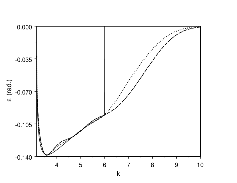
Figure 3: The mixing parameter $\varepsilon$. See Fig. 1 for details.

The “bound” parameters $\left\{\lambda_{1},\,Z_{N,1},\,Z_{\mathcal{N},1}\right\}$ and the “external” ones $\left\{\lambda_{j},\,Z_{N,j},\,Z_{\mathcal{N},j}\right\}$, $j=9,\,10$ are found by solving the system that consists of (42), (43), (48), (50). In the calculations of $a^{(1)}_{N-1}$, $a^{(2)}_{N-1}$, $u_{N-1}$ in Eq. (43) the approximations (44), (47) have been applied. The resulting parameters $\left\{\lambda_{j},\,Z_{N,j},\,Z_{\mathcal{N},j}\right\}$ are presented in Table I (a). Table III(a) lists the corresponding Hamiltonian matrix (8). In Figs. 1-3 are shown the eigenphase shifts $\delta_{1}$, $\delta_{2}$ and the mixing parameter $\varepsilon$ corresponding to the matrix ${\bf S}(k)$ in the integrands on the right-hand side of (56) (thin solid line) and the resulting matrix ${\bf S}^{(0)}(k)$ (dashed line).

In order to evaluate the effect of the closed channel the iteration procedure described in the previous section is applied. The convergence of $a^{(1)}_{N-1}$, $a^{(2)}_{N-1}$, $u_{N-1}$ on the left-hand side of (43) depending on the number of iterations is displayed in Table II. The resulting parameters $\left\{\lambda_{j},\,Z_{N,j},\,Z_{\mathcal{N},j}\right\}$, ($j=1,\,9,\,10$) and the Hamiltonian matrix (8) after 5 steps are listed in Tables I(b) and Table III(b), respectively. The eigenphase shifts $\delta_{1}$, $\delta_{2}$ and the mixing parameter $\varepsilon$ corresponding to the matrix ${\bf S}^{(5)}(k)$ are plotted in Figs. 1-3 (dotted line).

A comparison of (a) and (b) results shows that, as we might expect, the off-diagonal part $V^{(12)}=V^{(21)}$ of the interaction (1), (2) is most sensitive to the used approximations. The mixing parameter $\varepsilon$ behavior (see Figs. 3) reflects this dependence. Notice that the difference in the mixing parameters (in the interval $[0,\,k_{0}]$) is within the accuracy of the method.

V Conclusion

A generalization of the $J$-matrix inverse scattering approach to the case of two coupled channels with different threshold energies has been discussed. All the modification introduced in the inverse scheme TMP ; PRCJ (employed in the case of a two-channel system without threshold) appear to be plane and relatively obvious. An inverse procedure is proposed which focuss on reproducing the scattering data in a given energy interval. On the other hand, the procedure allows us to evaluate the contribution from the closed channel to the sought-for potential.

Appendix A The $J$-matrix version of the Marchenko equations

$f_{n}^{(\alpha\,\beta)}$ (as well as $\mathcal{C}_{n\,\ell_{\alpha}}^{(\pm)}$) satisfies the three-term recursion relations (12). It follows herefrom, in view of the boundary conditions (10), (14) and the Hamiltonian matrix quasitridiagonal form (8), that the coefficients $c_{n}^{(\alpha\beta)}(k)$, $c_{n}^{(\alpha\beta)}(\nu)$ can be expressed as

$$c_{n}^{(\alpha\,\beta)}=\sum\limits_{\begin{subarray}{c}m=n\\ \gamma=1,2\end{subarray}}^{2N-n-2}K_{n\,m}^{(\alpha\,\gamma)}f_{m}^{(\gamma\,\beta)}.$$ (51)

Besides, (10), (14) imply that $K_{N-1,N-1}^{(\alpha\,\beta)}=\delta_{\alpha\,\beta}$. Further, from the expansion (51) and the completeness relations (16) it follows that ${\bf c}_{n}$ is orthogonal to every ${\bf f}_{m}$ for $n<m$, i. e.

$$\frac{2}{\pi}\int\limits_{0}^{\infty}dk\,{\bf c}_{n}(k)\,{\bf P}\,{{\bf f}_{m}(k)}^{{\dagger}}+\sum\limits_{\nu}{\bf c}_{n}^{(\nu)}{\bf A}_{\nu}{{\bf f}_{m}^{(\nu)}}^{{\dagger}}={\bf 0},\qquad m>n,$$ (52)

where

$${\bf f}_{n}(k)=\left(\begin{array}[]{cc}f_{n}^{(11)}(k)&f_{n}^{(12)}(k)\\ f_{n}^{(21)}(k)&f_{n}^{(22)}(k)\\ \end{array}\right),\qquad{\bf f}_{n}^{(\nu)}=\left(\begin{array}[]{cc}f_{n}^{(1)}(\nu)&0\\ 0&f_{n}^{(2)}(\nu)\\ \end{array}\right).$$ (53)

Inserting the expansion (51) into (52) and (16) then yields

$$\sum\limits_{n^{\prime}=n}^{2N-n-2}{\bf K}_{n\,n^{\prime}}{\bf Q}_{n^{\prime}\,m}={\bf 0},\quad m>n,$$ (54)

$$\sum\limits_{m=n}^{2N-n-2}{\bf K}_{n\,m}{\bf Q}_{m\,n}\widetilde{\bf K}_{n\,n}={\bf I},$$ (55)

where

$${\bf Q}_{n\,m}=\frac{2}{\pi}\int\limits_{0}^{\infty}dk\,{\bf f}_{n}(k)\,{\bf P}\,{{\bf f}_{m}(k)}^{{\dagger}}+\sum\limits_{\nu}{\bf f}_{n}^{(\nu)}{\bf A}_{\nu}{{\bf f}_{m}^{(\nu)}}^{{\dagger}},$$ (56)

$${\bf K}_{n\,m}=\left(\begin{array}[]{cc}K^{(11)}_{n\,m}&K^{(12)}_{n\,m}\\ K^{(21)}_{n\,m}&K^{(22)}_{n\,m}\\ \end{array}\right).$$ (57)

Setting

$${\bf K}_{n\,m}={\bf K}_{n\,n}{\bf M}_{n\,m},\quad m>n,$$ (58)

we can rewrite (54) in the form

$$\sum\limits_{n^{\prime}=n+1}^{2N-n-2}{\bf M}_{n\,n^{\prime}}{\bf Q}_{n^{\prime}\,m}=-{\bf Q}_{n\,m},\quad m>n.$$ (59)

Inserting (58) in (55) gives

$$\widetilde{\bf K}_{n\,n}{\bf K}_{n\,n}=\left[{\bf Q}_{n\,n}+\sum\limits_{m=n+1}^{2N-n-2}{\bf M}_{n\,m}{\bf Q}_{m\,n}\right]^{-1}.$$ (60)

Once ${\bf M}_{n\,m}$ have been found by solving (59), ${\bf K}_{n\,n}$ can be evaluated from (60). Notice that in this case the Hamiltonian matrix quasitridiagonal form (8) implies that $K_{n\,n}^{(21)}=0$.

A knowledge of $K_{n\,m}^{(\alpha\,\beta)}$ finally furnishes the Hamiltonian matrix (8) according to

$$\begin{array}[]{c}a_{n}^{(1)}=T_{n\,n}^{(1)}+\frac{K^{(11)}_{n\,n+1}}{K^{(11)}_{n\,n}}T_{n+1,\,n}^{(1)}-\frac{K^{(12)}_{n,\,n}\,K^{(21)}_{n-1,\,n}}{K^{(11)}_{n,\,n}K^{(22)}_{n-1,\,n-1}}T_{n,\,n-1}^{(2)}-\\[11.38109pt] \qquad\qquad\qquad\qquad\qquad-\left(\frac{K^{(11)}_{n-1,\,n}}{K^{(11)}_{n-1,\,n-1}}-\frac{K^{(12)}_{n-1,\,n-1}K^{(21)}_{n-1,\,n}}{K^{(11)}_{n-1,\,n-1}\,K^{(22)}_{n-1,\,n-1}}\right)T_{n,\,n-1}^{(1)},\end{array}$$ (61)

$$b^{(1)}_{n}=\frac{K^{(11)}_{n,\,n}}{K^{(11)}_{n-1,\,n-1}}T_{n,\,n-1}^{(1)},$$ (62)

$$\begin{array}[]{c}a_{n}^{(2)}=T_{n\,n}^{(2)}+\frac{\rho^{2}}{2}\Delta+\frac{K^{(22)}_{n\,n+1}}{K^{(22)}_{n\,n}}T_{n+1,\,n}^{(2)}-\frac{K^{(12)}_{n,\,n}\,K^{(21)}_{n,\,n+1}}{K^{(11)}_{n,\,n}\,K^{(22)}_{n,\,n}}T_{n+1,\,n}^{(1)}-\\[11.38109pt] \qquad\qquad\qquad\qquad\qquad-\left(\frac{K^{(22)}_{n-1,\,n}}{K^{(22)}_{n-1,\,n-1}}-\frac{K^{(12)}_{n,\,n}\,K^{(21)}_{n-1,\,n}}{K^{(11)}_{n,\,n}\,K^{(22)}_{n-1,\,n-1}}\right)T_{n,\,n-1}^{(2)},\end{array}$$ (63)

$$b^{(2)}_{n}=\frac{K^{(22)}_{n,\,n}}{K^{(22)}_{n-1,\,n-1}}T_{n,\,n-1}^{(2)},$$ (64)

$$u_{n}=\frac{K^{(21)}_{n,\,n+1}}{K^{(11)}_{n,\,n}}T_{n+1,\,n}^{(1)}-\frac{K^{(21)}_{n-1,\,n}\,K^{(22)}_{n,\,n}}{K^{(11)}_{n,\,n}\,K^{(22)}_{n-1,\,n-1}}T_{n,\,n-1}^{(2)},$$ (65)

$$v_{n}=\frac{K^{(12)}_{n,\,n}}{K^{(22)}_{n-1,\,n-1}}T_{n,\,n-1}^{(2)}-\frac{K^{(12)}_{n-1,\,n-1}\,K^{(11)}_{n,\,n}}{K^{(22)}_{n-1,\,n-1}\,K^{(11)}_{n-1,\,n-1}}T_{n,\,n-1}^{(1)}.$$ (66)

Table 1: The eigenvalues and the eigenvector components of the Hamiltonian matrix (8).

$j$		$\lambda_{j}$	$Z_{N,j}$	$Z_{\mathcal{N},j}$
1	(a) (b)	-0.58970264603 -0.58970263847	-0.012333185006 -0.012333362733	0.00018915595025 0.00019663447693
2		0.40533438179	0.18715853083	0
3		0.78492505414	0.090561490976	0
4		1.5244162751	0.32069508364	0.068124022185
5		1.6473065387	0.14429242884	-0.17954224586
6		2.6728511248	0.056915520013	0.34337676573
7		3.2807264076	0.50263953170	-0.052996407816
8		4.3839439596	0.050257472502	0.49798274116
9	(a) (b)	6.3135416565 6.3156804888	0.75676372010 0.75741514694	-0.062001763734 -0.048160786961
10	(a) (b)	7.5694793828 7.5651078745	-0.043006216886 -0.029379475185	-0.76848969549 -0.76948110211

Table 2: Convergence of $a^{(1)}_{N-1}$, $a^{(2)}_{N-1}$, $u_{N-1}$ on the left-hand side of (43). $i$ is the number of iterations.

$i$	$a_{N-1}^{(1)}$	$a_{N-1}^{(2)}$	$u_{N-1}$
0	4.689928491	5.966326902	0.0191266184
1	4.689911469	5.965705556	0.0071475853
2	4.689912701	5.965663226	0.0059643414
3	4.689912839	5.965658934	0.0058474387
4	4.689912852	5.965658510	0.0058359055
5	4.689912854	5.965658464	0.0058347978

Table 3: The elements of the Hamiltonian matrix (8).

$n$	$a_{n}^{(1)}$	$b_{n}^{(1)}$	$a_{n}^{(2)}$	$b_{n}^{(2)}$	$u_{n}$	$v_{n}$
(a)
0	0.1775666649		0.06753394526		0.6517927001
1	1.212316541	-0.3078456533	2.378081035	-0.01876213797	0.03459618331	0.1112824167
2	2.233751540	-0.8637975100	3.353299231	-0.7967451984	0.02226447163	-0.06006980906
3	3.357567064	-1.370400686	4.556450725	-1.319787140	0.04861624566	-0.07835689367
4	4.689928491	-2.007758312	5.966326902	-2.032477517	0.0191266184	-0.06589047115
(b)
0	0.2553490884		-0.01023393318		0.6404835124
1	1.212396865	-0.3006058502	2.378394045	-0.01965488685	0.03937726990	0.1295217295
2	2.233837107	-0.8638658833	3.353460226	-0.7967777718	0.02976290436	-0.06151639336
3	3.357902488	-1.370738931	4.553912267	-1.319081324	0.04174355881	-0.07598084688
4	4.689912854	-2.008020573	5.965658464	-2.031439617	0.0058347978	-0.04479790470

Figure 1: The eigenphase shift $\delta_{1}$ corresponding to the matrix ${\bf S}(k)$ on the right-hand side of (56) (thin solid line) and the resulting matrices: ${\bf S}^{(0)}(k)$ (dashed line) and ${\bf S}^{(5)}(k)$ (dotted line).

Figure 2: The eigenphase shift $\delta_{2}$. See Fig. 1 for details.

References

- (1) H. A. Yamani, L. Fishman, J. Math. Phys. 16, 410 (1975).
- (2) J. T. Broad, W. P. Reinhardt, J. Phys. B 9, 1491 (1976).
- (3) S. A. Zaitsev, Teoret. Math. Phys. 121, 424 (1999).
- (4) S. A. Zaitsev, E. I. Kramar, J. Phys. G, 27, 2037 (2001).
- (5) A. M. Shirokov, A. I. Mazur, S. A. Zaytsev, J. P. Vary, T. A. Weber, Phys. Rev. C 70 (2004) 044005.
- (6) A. I. Baz, Ya. B. Zeldovitch and A. M. Perelomov, Scattering, Reactions and Decays in Non-relativistic Quantum Mechanics (Moscow: Nauka, 1971).
- (7) K. Chadan, P. C. Sabatier, Inverse Problems in Quantum Scattering Theory (New York, Heidelberg, Berlin: Springer-Verlag, 1977).
- (8) S. A. Zaytsev, IP 21 (2005) 1061.
- (9) A. M. Shirokov, Yu. F. Smirnov, and S. A. Zaytsev, Teor. Mat. Fiz. 117, 227 (1998) [Theor. Math. Phys. 117, 1291 (1998)].
- (10) B. F. Samsonov, J.-M. Sparenberg, D. Baye, J. Phys. A 40 (2007) 4225.