Jeans type analysis of chemotactic collapse

Abstract

We perform a linear dynamical stability analysis of a general hydrodynamic model of chemotactic aggregation [Chavanis & Sire, Physica A, 384, 199 (2007)]. Specifically, we study the stability of an infinite and homogeneous distribution of cells against “chemotactic collapse”. We discuss the analogy between the chemotactic collapse of biological populations and the gravitational collapse (Jeans instability) of self-gravitating systems. Our hydrodynamic model involves a pressure force which can take into account several effects like anomalous diffusion or the fact that the organisms cannot interpenetrate. We also take into account the degradation of the chemical which leads to a shielding of the interaction like for a Yukawa potential. Finally, our hydrodynamic model involves a friction force which quantifies the importance of inertial effects. In the strong friction limit, we obtain a generalized Keller-Segel model similar to the generalized Smoluchowski-Poisson system describing self-gravitating Langevin particles. For small frictions, we obtain a hydrodynamic model of chemotaxis similar to the Euler-Poisson system describing a self-gravitating barotropic gas. We show that an infinite and homogeneous distribution of cells is unstable against chemotactic collapse when the “velocity of sound” in the medium is smaller than a critical value. We study in detail the linear development of the instability and determine the range of unstable wavelengths, the growth rate of the unstable modes and the damping rate, or the pulsation frequency, of the stable modes as a function of the friction parameter and shielding length. For specific equations of state, we express the stability criterion in terms of the density of cells.

Key words: Nonlinear mean field Fokker-Planck equations, generalized thermodynamics, chemotaxis, gravity, long-range interactions

1 Introduction

In biology, many microscopic organisms (bacteria, amoebae, endothelial cells,…) or even social insects (like ants) interact through the phenomenon of chemotaxis [1]. These organisms deposit a chemical (pheromone, smell, food,…) that has an attractive effect on the organisms themselves. Therefore, in addition to their diffusive motion, they move preferentially along the gradient of concentration of the chemical they secrete (chemotactic flux). When chemotactic attraction prevails over diffusion, this process can lead to a “chemotactic collapse” (see [2] for a review) resulting in the aggregation of the organisms. In this way, some structures can form like clusters (clumps) or even network patterns (filaments). Therefore, the chemotactic interaction can explain several features of the morphogenesis of biological colonies. The chemotactic aggregation of biological populations is usually described in terms of the Keller-Segel model [3]. This is a parabolic model consisting in two coupled differential equations. The first equation is a drift-diffusion equation describing the evolution of the concentration of cells and the second equation is a reaction-diffusion equation with terms of source and degradation describing the evolution of the concentration of the secreted chemical. This model ignores inertial effects and assumes that the drift velocity of the organisms is directly induced by a chemotactic “force” proportional to the concentration gradient of the chemical. The Keller-Segel model can reproduce the formation of clusters (clumps) by chemotactic collapse [4-19]. This reflects experiments on bacteria like Escherichia coli or amoebae like Dictyostelium discoïdeum exhibiting pointwise concentration [3]. However, parabolic models fail at describing the formation of network patterns (filaments). These filaments are observed in experiments of capillary blood vessels formation [20]. They correspond to the spontaneous self-organization of endothelial cells during vasculogenesis, a process occuring during embryologic development. In order to account for these structures, more general models of chemotaxis have been introduced [21, 22, 23]. They have the form of hydrodynamic (hyperbolic) models taking into account inertial effects. These models can reproduce the formation of filaments that are interpreted as the beginning of a vasculature. This phenomenon is responsible of angiogenesis, a major factor for the growth of tumors [24]. Interestingly, these filaments share some analogies with the large-scale structures in the universe that are described by similar hydrodynamic equations [25, 26].

Recently, we have introduced a general kinetic model of chemotactic aggregation based on generalized stochastic processes, non linear mean field Fokker-Planck equations and generalized thermodynamics [23]. From these kinetic equations, we have derived a hydrodynamic model of the form

(1) $${\partial\rho\over\partial t}+\nabla\cdot(\rho{\bf u})=0,$$

(2) $$\frac{\partial{\bf u}}{\partial t}+({\bf u}\cdot\nabla){\bf u}=-{1\over\rho}\nabla p+\nabla c-\xi{\bf u},$$

(3) $${\partial c\over\partial t}=D_{c}\Delta c-kc+h\rho.$$

It involves a pressure force $-\nabla p$, where $p=p(\rho)$ is a barotropic equation of state that can take into account several effects like anomalous diffusion or the fact that the particles do not interpenetrate. It also involves a friction force $-\xi{\bf u}$ which measures the importance of inertial effects. For $\xi=0$, we recover the hyperbolic model introduced by Gamba et al. [21]. For $\xi\rightarrow+\infty$, we can neglect the inertial term in the momentum equation (2) leading to $\xi{\bf u}\simeq-{1\over\rho}\nabla p+\nabla c$ (overdamped limit). Substituting this relation in the equation of continuity (1), we obtain the generalized Keller-Segel model

(4) $${\partial\rho\over\partial t}=\nabla\cdot\left[\chi\left(\nabla p-\rho\nabla c\right)\right],$$

(5) $${\partial c\over\partial t}=D_{c}\Delta c-kc+h\rho,$$

where $\chi=1/\xi$. Interestingly, this model of chemotaxis is similar to a model of self-gravitating Langevin particles [27] described by the damped Euler-Poisson system

(6) $${\partial\rho\over\partial t}+\nabla\cdot(\rho{\bf u})=0,$$

(7) $$\frac{\partial{\bf u}}{\partial t}+({\bf u}\cdot\nabla){\bf u}=-{1\over\rho}\nabla p-\nabla\Phi-\xi{\bf u},$$

(8) $$\Delta\Phi=S_{d}G\rho.$$

For $\xi=0$, it reduces to the barotropic Euler-Poisson system [28] and for $\xi\rightarrow+\infty$, we obtain the generalized Smoluchowski-Poisson system

(9) $${\partial\rho\over\partial t}=\nabla\cdot\left[\frac{1}{\xi}\left(\nabla p+\rho\nabla\Phi\right)\right],$$

(10) $$\Delta\Phi=S_{d}G\rho.$$

In this analogy, we see that the concentration $-c({\bf r},t)$ of the chemical plays the same role as the gravitational potential $\Phi({\bf r},t)$. In biology, the interaction is mediated by a material substance (the secreted chemical) while the physical interpretation of the gravitational potential in astrophysics is more abstract . The hydrodynamic equations (1)-(5) or (6)-(10) involving a barotropic equation of state, a long-range potential of interaction and a friction force, have been introduced by Chavanis [29, 30] at a general level. It was indicated that they could provide generalized models of chemotaxis and self-gravitating Brownian particles.

The main difference between the chemotactic model (1)-(5) and the gravitational model (6)-(10) concerns the field equations (3) and (8). In astrophysics, the gravitational potential is determined instantaneously from the density of particles through the Poisson equation (8). In biology, the equation (3) determining the evolution of the chemical is more complex and involves memory terms. The chemical diffuses with a diffusion coefficient $D_{c}$, is produced by the organisms at a rate $h$ and is degraded at a rate $k$. Because of the term $\partial c/\partial t$, the concentration of the chemical at time $t$ depends on the concentration of the organisms at earlier times. In this paper, we shall consider simplified models where the term $\partial c/\partial t$ can be neglected. This is valid in a limit of large diffusivity of the chemical $D_{c}\rightarrow+\infty$ [6]. We first consider the case where there is no degradation of the chemical ($k=0$). Then, assuming $h=\lambda D_{c}$ and taking the limit $D_{c}\rightarrow+\infty$ with $\lambda=O(1)$, one gets (see Appendix C of [23])

(11) $$\Delta c=-\lambda(\rho-\overline{\rho}),$$

where $\overline{\rho}=(1/V)\int\rho d{\bf r}=M/V$ is the average value of the density which is a conserved quantity. In that case, the concentration of the chemical is given by a Poisson equation which incorporates a sort of “neutralizing background” (played by $\overline{\rho}$) like in the Jellium model of plasma physics [31]. Note that a similar term also arises in cosmology when we take into account the expansion of the universe and work in a comoving system of coordinates [25]. We shall thus refer to this model as the “Newtonian model”. Then, we consider the case of a finite degradation rate. Assuming $h=\lambda D_{c}$, $k=k_{0}^{2}D_{c}$ and taking the limit $D_{c}\rightarrow+\infty$ with $\lambda=O(1)$ and $k_{0}=O(1)$, one gets (see Appendix C of [23])

(12) $$\Delta c-k_{0}^{2}c=-\lambda\rho.$$

If we take formally $k_{0}=0$, we obtain a Poisson equation similar to Eq. (8) where $-c({\bf r},t)$ plays the role of $\Phi({\bf r},t)$ and $\lambda$ plays the role of the gravitational constant $S_{d}G$ (we recall that the geometrical factor $S_{d}$ is the surface of a unit sphere in $d$ dimensions). However, Eq. (12) has been derived for $k_{0}\neq 0$ (for $k_{0}=0$ we get Eq. (11)). This implies that the interaction is shielded on a typical distance $k_{0}^{-1}$. This is similar to the Debye shielding in plasma physics, to the Rossby shielding in geophysical flows or to the Yukawa shielding in nuclear physics. We shall refer to this model as the “Yukawa model”.

In this paper, we perform a detailed linear dynamical stability analysis of the chemotactic model (1)-(3). Specifically, we study the stability of an infinite and homogeneous distribution of cells against chemotactic collapse. This is similar to the classical Jeans stability analysis for the barotropic Euler-Poisson system [28]. Indeed, the “chemotactic collapse” of biological populations is similar to the “gravitational collapse” in astrophysics (Jeans instability). There are, however, two main differences with the classical Jeans analysis. The first difference is the presence of a friction force $-\xi{\bf u}$ in the Euler equation. As we shall see, this does not change the onset of the instability but this affects the evolution of the perturbation. The second difference arises from the different nature of the field equations (3) and (8). We recall that, in gravitational dynamics, an infinite and homogeneous distribution of matter with $\rho=cst$ and ${\bf u}={\bf 0}$ is not a stationary solution of the barotropic Euler-Poisson system (6)-(8) because we cannot satisfy simultaneously the condition of hydrostatic equilibrium $\nabla p(\rho)+\rho\nabla\Phi={\bf 0}$ reducing to $\nabla\Phi={\bf 0}$ and the Poisson equation $\Delta\Phi=S_{d}G\rho\neq 0$. This leads to an inconsistency in the mathematical analysis when studying the linear dynamical stability of such a distribution: this is called the “Jeans swindle” [28] . By contrast, there is no “Jeans swindle” in the chemotactic problem! Indeed, an infinite and homogeneous distribution of cells is a steady state of the equations of motion (1)-(3) corresponding to the condition $kc=h\rho$. For the “Newtonian model” (11), this condition becomes $\rho=\overline{\rho}$ and for the “Yukawa model” (12), it becomes $k_{0}^{2}c=\lambda\rho$.

In this paper, we study in detail the onset of the “chemotactic instability” and its development in the linear regime. This study was initiated in [34] at a general level, i.e. taking into account the term $\partial c/\partial t$ in Eq. (3) and allowing the coefficients in Eqs. (1)-(3) to depend on the concentration. However, this study focused on the unstable modes and did not analyze in detail the evolution of the stable modes. In the present paper, we make a complete study of both stable and unstable modes but we restrict ourselves to the simplified models (11) and (12). In the “Newtonian model” (11), the only difference with the Jeans analysis is the presence of the friction force $\xi$. In the “Yukawa model” (12), the differences with the Jeans analysis are due to the effects of the friction $\xi$ and of the shielding length $k_{0}^{-1}$ generated by the degradation of the chemical. We show that the system is always stable for

(13) $$c_{s}\geq(c_{s})_{crit}\equiv\left(\frac{\lambda\overline{\rho}}{k_{0}^{2}}\right)^{1/2},$$

where $c_{s}\equiv(dp/d\rho)^{1/2}$ is the “velocity of sound” in the medium (for specific equations of state, discussed in Sec. 4, we can express the stability criterion (13) in terms of the density of cells). Therefore, the system is stable if the velocity of sound is above a certain threshold fixed by the shielding length $k_{0}$. By contrast, for $c_{s}<(c_{s})_{crit}$, the system is unstable for wavenumbers

(14) $$k\leq k_{m}\equiv\sqrt{k_{J}^{2}-k_{0}^{2}},$$

where $k_{J}=(\lambda\overline{\rho}/c_{s}^{2})^{1/2}$ is the Jeans wavenumber. In the Newtonian model, the condition $k_{0}=0$ implies $(c_{s})_{crit}=+\infty$, so that the system is always unstable to perturbations with sufficiently large wavelengths $k<k_{J}$. These results are independent on $\xi$. The friction term only affects the evolution of the perturbation. For $k<k_{m}(k_{0})$, the perturbation grows exponentially rapidly, for $k_{m}(k_{0})<k<k_{c}(\xi,k_{0})$ (where $k_{c}$ is a friction-dependent wavenumber defined in the text) it is damped exponentially rapidly without oscillating and for $k>k_{c}(\xi,k_{0})$ it presents damped oscillations. More precisely, we determine the growth rate of the unstable modes and the damping rate, and oscillation frequency, of the stable modes as a function of $\xi$ and $k_{0}^{-1}$. Owing to the above mentioned analogy between chemotaxis and gravity, our stability analysis also applies to self-gravitating Langevin particles [27] provided that we make the “Jeans swindle”.

2 Jeans-type instability for a Newtonian potential

In this section, we study the linear dynamical stability of an infinite and homogeneous stationary solution of the fluid equations

(15) $$\frac{\partial\rho}{\partial t}+\nabla\cdot(\rho{\bf u})=0,$$

(16) $${\partial{\bf u}\over\partial t}+({\bf u}\cdot\nabla){\bf u}=-{1\over\rho}\nabla p+\nabla c-\xi{\bf u},$$

(17) $$\Delta c=-\lambda(\rho-\overline{\rho}).$$

We consider an infinite and homogeneous distribution of cells $\rho=\overline{\rho}$, with no velocity ${\bf u}={\bf 0}$ and no chemical $c=0$. This is an exact stationary solution of the fluid equations (15)-(17). Linearizing Eqs. (15)-(17) around this steady state and writing the perturbation in the form $\delta f({\bf r},t)\sim e^{i({\bf k}\cdot{\bf r}-\omega t)}$, we readily obtain the dispersion relation [27]:

(18) $$\omega(\omega+i\xi)=c_{s}^{2}k^{2}-\lambda\overline{\rho},$$

where we have introduced the equivalent of the velocity of sound $c_{s}^{2}=p^{\prime}(\overline{\rho})$. Setting $\sigma=-i\omega$, so that $\delta f\propto e^{\sigma t}$, the dispersion relation can be rewritten

(19) $$\sigma^{2}+\xi\sigma+c_{s}^{2}k^{2}-\lambda\overline{\rho}=0.$$

The solutions are $\sigma_{\pm}=(-\xi\pm\sqrt{\Delta})/2$ with $\Delta(k)=\xi^{2}-4(c_{s}^{2}k^{2}-\lambda\overline{\rho})$. If $c_{s}^{2}k^{2}-\lambda\overline{\rho}<0$, then $\Delta>\xi^{2}>0$ and the system is unstable since $\sigma_{+}=(-\xi+\sqrt{\Delta})/2>0$. If $c_{s}^{2}k^{2}-\lambda\overline{\rho}>0$, either (i) $\Delta<0$ implying $R_{e}(\sigma)=-\xi/2$ or (ii) $0<\Delta<\xi^{2}$, implying $\sigma_{\pm}<0$, so the system is stable. Therefore, the system is unstable if

(20) $$k<\left({\lambda\overline{\rho}\over c_{s}^{2}}\right)^{1/2}\equiv k_{J},$$

and stable otherwise. The critical value $k_{J}$ is similar to the Jeans wavenumber in astrophysics. We note that the threshold of instability does not depend on the friction parameter $\xi$. Note also that for negative chemotaxis (chemorepulsion) obtained by replacing $+\nabla c$ by $-\nabla c$ in Eq. (16), an infinite and homogeneous distribution of particles is always stable.

If we consider the case $\xi=0$ (Euler), the fluid equations (15)-(17) are similar to the Euler-Poisson system and the dispersion relation becomes

(21) $$\omega^{2}=c_{s}^{2}k^{2}-\lambda\overline{\rho}.$$

For $k>k_{J}$, the perturbation undergoes undamped oscillations with pulsation $\omega=c_{s}(k^{2}-k_{J}^{2})^{1/2}$. For $k<k_{J}$, the perturbation increases exponentially rapidly with a growth rate $\gamma=c_{s}(k_{J}^{2}-k^{2})^{1/2}$. For $c_{s}=0$, $k_{J}\rightarrow+\infty$ and the system is unstable for all wavenumbers. The growth rate of the perturbation is $\gamma=\sqrt{\lambda\overline{\rho}}$ independent on $k$. For $c_{s}\rightarrow+\infty$, $k_{J}\rightarrow 0$ and the system is stable for all wavenumbers. The pulsation is $\omega=c_{s}k$. If we now consider the case $\xi\rightarrow+\infty$ (Smoluchowski), the fluid equations (15)-(17) reduce to the generalized Smoluchowski-Poisson system

(22) $$\frac{\partial\rho}{\partial t}=\nabla\cdot\left[\frac{1}{\xi}(\nabla p-\rho\nabla c)\right],$$

(23) $$\Delta c=-\lambda(\rho-\overline{\rho}),$$

and the dispersion relation becomes

(24) $$i\xi\omega=c_{s}^{2}k^{2}-\lambda\overline{\rho}.$$

For $k>k_{J}$, the perturbation decays exponentially rapidly with a damping rate $\gamma=-{c_{s}^{2}}(k^{2}-k_{J}^{2})/\xi$. For $k<k_{J}$, the perturbation increases exponentially rapidly with a growth rate $\gamma={c_{s}^{2}}(k_{J}^{2}-k^{2})/\xi$. For $c_{s}=0$, $k_{J}\rightarrow+\infty$ and the system is unstable for all wavenumbers. The growth rate of the perturbation is $\gamma=\lambda\overline{\rho}/\xi$ independent on $k$. For $c_{s}\rightarrow+\infty$, $k_{J}\rightarrow 0$ and the system is stable for all wavenumbers. The damping rate is $\gamma=-c_{s}^{2}k^{2}/\xi$.

Let us now consider the general case of an arbitrary friction. There are two relevant wavenumbers in the problem: the Jeans wavenumber (20) and the wavenumber

(25) $$k_{c}\equiv\left(k_{J}^{2}+k_{d}^{2}\right)^{1/2},$$

where

(26) $$k_{d}\equiv{\xi\over 2c_{s}},$$

is a wavenumber constructed with the friction coefficient and the velocity of sound. We can define a dimensionless number

(27) $$F=\left(\frac{k_{d}}{k_{J}}\right)^{2}=\frac{\xi^{2}}{4\lambda\overline{\rho}},$$

which measures the strength of the friction force (a similar parameter was introduced in [27] for inhomogeneous distributions). It is independent on the equation of state $p(\rho)$ and it can be written $F\sim(\xi t_{D})^{2}$ where $t_{D}\sim 1/\sqrt{\overline{\rho}\lambda}$ is a typical dynamical time. Thus, $\sqrt{F}$ is the ratio of the dynamical time on the friction time $\tau\sim 1/\xi$. In terms of this parameter, the wavenumber (25) can be written $k_{c}=k_{J}\sqrt{1+F}$. The behaviour of the perturbation can be analyzed in terms of these wavenumbers: (i) If $\Delta<0$, the perturbation undergoes damped oscillations with pulsation $\omega=c_{s}(k^{2}-k_{c}^{2})^{1/2}$ and decay rate $\gamma=-\xi/2$. This stable regime corresponds to wavenumbers $k>k_{c}$. (ii) If $0<\Delta<\xi^{2}$, the perturbation decays exponentially rapidly with a damping rate $\gamma=-\xi/2+c_{s}(k_{c}^{2}-k^{2})^{1/2}$ without oscillating. This stable regime corresponds to wavenumbers $k_{J}<k<k_{c}$. For $k=k_{J}$, we have $\gamma=0$ and for $k=k_{c}$, we have $\gamma=-\xi/2$. (iii) If $\Delta>\xi^{2}$, the perturbation increases exponentially rapidly with a growth rate $\gamma=-\xi/2+c_{s}(k_{c}^{2}-k^{2})^{1/2}$. This unstable regime corresponds to wavenumbers $k<k_{J}$. The growth rate is maximum for $k_{*}=0$ and its value is $\gamma_{*}=-\xi/2+c_{s}k_{c}$. These results are summarized in Fig. 1.

Figure 1: In summary, a homogeneous distribution is unstable for $k<k_{J}$ and stable for $k>k_{J}$. For $k<k_{J}$, the perturbation grows exponentially rapidly. For $k_{J}<k<k_{c}$, the perturbation is damped exponentially rapidly without oscillating. For $k>k_{c}$, the perturbation undergoes damped oscillations. We have taken $F=1$, $k_{J}=1$ and $\xi=2$.

It is interesting to determine how the results depend on the friction parameter and on the velocity of sound. To simplify the notations, we define $T\equiv c_{s}^{2}$. Then, we obtain

(28) $$k_{J}(T)=\left({\lambda\overline{\rho}\over T}\right)^{1/2},$$

(29) $$k_{c}(T,\xi)=k_{J}(T)\sqrt{1+F},$$

(30) $$k_{*}=0,\qquad{2\over\xi}\gamma_{*}(\xi)=-1+\sqrt{1+{1\over F}}$$

(31) $${2\over\xi}\gamma(k,T,\xi)=-1+\sqrt{1+{1\over F}}\left[1-\left({k\over k_{c}}\right)^{2}\right]^{1/2},\qquad(k<k_{c}).$$

(32) $${2\over\xi}\omega(k,T,\xi)=\sqrt{1+{1\over F}}\left[\left({k\over k_{c}}\right)^{2}-1\right]^{1/2},\qquad\gamma=-\xi/2,\qquad(k>k_{c}).$$

For $T=0$, we find that $k_{J}\rightarrow+\infty$ so that the system is unstable for all wavenumbers. The growth rate of the perturbation is

(33) $${2\gamma\over\xi}=-1+\sqrt{1+{1\over F}},$$

independent on $k$. For $T\rightarrow+\infty$, if $\xi$ is finite, we get $k_{J}=k_{c}=0$ so that the system is stable for all wavenumbers. The pulsation is $\omega=\sqrt{T}k$ and the damping rate $\gamma=-\xi/2$.

For $\xi=0$, we find that $k_{c}=k_{J}$ and

(34) $$\gamma(k,T)=\sqrt{\lambda\overline{\rho}}\left[1-\left({k\over k_{J}}\right)^{2}\right]^{1/2},\qquad(k<k_{J})$$

(35) $$\omega(k,T)=\sqrt{\lambda\overline{\rho}}\left[\left({k\over k_{J}}\right)^{2}-1\right]^{1/2},\qquad\gamma=0,\qquad(k>k_{J}).$$

These results are summarized in Fig. 2. For $T=0$, we find that $k_{J}\rightarrow+\infty$ so that the system is unstable for all wavenumbers. The growth rate of the perturbation is $\gamma=\sqrt{\lambda\overline{\rho}}$. For $T\rightarrow+\infty$, we get $k_{J}=0$ so that the system is stable for all wavenumbers. The pulsation is $\omega=\sqrt{T}k$.

Figure 2: The limit $\xi=0$. We have taken $k_{J}=1$ and $\lambda\overline{\rho}=1$.

For $\xi\rightarrow+\infty$, we find that $k_{c}\rightarrow+\infty$ and

(36) $$\gamma(k,T)={\lambda\overline{\rho}\over\xi}\left(1-{k^{2}\over k_{J}^{2}}\right).$$

These results are summarized in Fig. 3. For $T=0$, we find that $k_{J}\rightarrow+\infty$ so that the system is unstable for all wavenumbers. The growth rate of the perturbation is $\gamma={\lambda\overline{\rho}/\xi}$. For $T\rightarrow+\infty$, we get $k_{J}=0$ so that the system is stable for all wavenumbers. The damping rate is $\gamma=-{T}k^{2}/\xi$.

Figure 3: The limit $\xi\rightarrow+\infty$. We have taken $k_{J}=1$ and $\lambda\overline{\rho}=1$

If we now consider the stability problem of Eqs. (15)-(17) in a two-dimensional periodic domain of size $L$, the wavenumbers can be written ${\bf k}={2\pi\over L}(m,n)$ where $m$, $n$ are positive integers with $(m,n)\neq(0,0)$. In that case, the condition of instability (20) becomes

(37) $$m^{2}+n^{2}<{\lambda\overline{\rho}L^{2}\over 4\pi^{2}c_{s}^{2}}.$$

A necessary condition of instability is therefore $\lambda\overline{\rho}L^{2}/(4\pi^{2}c_{s}^{2})>1$. For an equation of state of the form $p(\rho)=\rho T$, where $T$ plays the role of a temperature, the velocity of sound is $c_{s}^{2}=T$ and the necessary condition of instability can be written

(38) $$T<T_{c}={\lambda\overline{\rho}L^{2}\over 4\pi^{2}},$$

where $T_{c}$ is a critical temperature. For $T>T_{c}$, there is no chemotactic collapse: the “gas” of cells remains spatially uniform and diffuse. For $T<T_{c}$, the distribution of cells is unstable and the number of unstable modes increases as $T$ decreases yielding more and more clusters. This instability has been illustrated numerically in [23] by solving the $N$-body equations of motion in a two-dimensional periodic domain.

3 Jeans-type instability criterion for a Yukawa potential

We now consider the linear dynamical stability of an infinite and homogeneous stationary solution of the fluid equations

(39) $$\frac{\partial\rho}{\partial t}+\nabla\cdot(\rho{\bf u})=0,$$

(40) $${\partial{\bf u}\over\partial t}+({\bf u}\cdot\nabla){\bf u}=-{1\over\rho}\nabla p+\nabla c-\xi{\bf u},$$

(41) $$\Delta c-k_{0}^{2}c=-\lambda\rho.$$

Comparing with Eq. (17), we see that the Laplacian is replaced by the operator $\Delta-k_{0}^{2}$. This implies that the interaction, mediated by the concentration $c$ of the chemical, is screened on a distance $k_{0}^{-1}$ where $k_{0}=(k/D_{c})^{1/2}$ [$k$ should not be confused here with the wavenumber]. A uniform distribution of cells and secreted chemicals whose concentrations satisfy the relation $k_{0}^{2}c=\lambda\overline{\rho}$ is an exact stationary solution of Eqs. (39)-(41). Considering a small perturbation around this steady state, we find that the dispersion relation replacing Eq. (19) is [27]:

(42) $$\sigma^{2}+\xi\sigma+k^{2}\left(c_{s}^{2}-{\lambda\overline{\rho}\over k^{2}+k_{0}^{2}}\right)=0.$$

The solutions are $\sigma_{\pm}=(-\xi\pm\sqrt{\Delta})/2$ with

(43) $$\Delta(k)=\xi^{2}-4k^{2}\left(c_{s}^{2}-{\lambda\overline{\rho}\over k^{2}+k_{0}^{2}}\right).$$

Repeating the arguments following Eq. (19), we find that the system is unstable if

(44) $$c_{s}^{2}<{\lambda\overline{\rho}\over k^{2}+k_{0}^{2}},$$

and stable otherwise. A necessary condition for instability is that

(45) $$c_{s}^{2}<(c_{s}^{2})_{crit}\equiv{\lambda\overline{\rho}\over k_{0}^{2}}.$$

When this condition is fulfilled, the range of unstable wavelengths is

(46) $$k\leq k_{m}\equiv\sqrt{k_{J}^{2}-k_{0}^{2}}.$$

We see that for $k_{0}\neq 0$, the instability is shifted to larger wavelengths than the Jeans length.

If we consider the case $\xi=0$ (Euler), the dispersion relation becomes

(47) $$\sigma^{2}=c_{s}^{2}k^{2}{k_{m}^{2}-k^{2}\over k_{0}^{2}+k^{2}}.$$

For $k>k_{m}$, the perturbation undergoes undamped oscillations with pulsation $\omega=\sqrt{-\sigma^{2}}$. For $k<k_{m}$, the perturbation increases exponentially rapidly with a growth rate $\gamma=\sqrt{\sigma^{2}}$. If we consider the case $\xi\rightarrow+\infty$ (Smoluchowski), the dispersion relation becomes

(48) $$\xi\sigma=c_{s}^{2}k^{2}{k_{m}^{2}-k^{2}\over k_{0}^{2}+k^{2}}.$$

For $k>k_{m}$, the perturbation decays exponentially rapidly with a damping rate $\gamma=\sigma<0$. For $k<k_{m}$, the perturbation increases exponentially rapidly with a growth rate $\gamma=\sigma>0$.

Figure 4: Growth rate and pulsation as a function of the wavenumber. We have taken $T/T_{c}=1/2$, $F=0.05$, $k_{0}=1$ and $\xi=2$

Let us now consider the general case of an arbitrary friction. We introduce a critical wavenumber $k_{c}$ defined by

(49) $$2k_{c}^{2}=k_{m}^{2}+k_{d}^{2}+\sqrt{(k_{m}^{2}+k_{d}^{2})^{2}+4k_{0}^{2}k_{d}^{2}}.$$

This expression generalizes Eq. (25) to the case $k_{0}\neq 0$. We also introduce the wavenumber $k_{s}$ defined by

(50) $$2k_{s}^{2}=-(k_{m}^{2}+k_{d}^{2})+\sqrt{(k_{m}^{2}+k_{d}^{2})^{2}+4k_{0}^{2}k_{d}^{2}}.$$

The behaviour of the perturbation can be analyzed in terms of these wavenumbers: (i) If $\Delta<0$, the perturbation undergoes damped oscillations with pulsation

(51) $$\omega={\xi\over 2}\sqrt{{k^{2}(k^{2}-k_{m}^{2})\over k_{d}^{2}(k^{2}+k_{0}^{2})}-1},$$

or equivalently

(52) $$\omega=c_{s}\left[\frac{(k^{2}-k_{c}^{2})(k^{2}+k_{s}^{2})}{k^{2}+k_{0}^{2}}\right]^{1/2},$$

and decay rate $\gamma=-\xi/2$. This stable regime corresponds to wavenumbers $k>k_{c}$. (ii) If $0<\Delta<\xi^{2}$, the perturbation decays exponentially rapidly with a damping rate

(53) $$\gamma=-{\xi\over 2}+{\xi\over 2}\sqrt{1-{k^{2}(k^{2}-k_{m}^{2})\over k_{d}^{2}(k^{2}+k_{0}^{2})}},$$

or equivalently

(54) $$\gamma=-{\xi\over 2}+c_{s}\left[{(k_{c}^{2}-k^{2})(k_{s}^{2}+k^{2})\over k^{2}+k_{0}^{2}}\right]^{1/2},$$

without oscillating. This stable regime corresponds to wavenumbers $k_{m}<k<k_{c}$. For $k=k_{c}$, we have $\gamma=-\xi/2$ and for $k=k_{m}$ we have $\gamma=0$. (iii) If $\Delta>\xi^{2}$, the perturbation increases exponentially rapidly with a growth rate $\gamma$ given by Eq. (53). This unstable regime corresponds to wavenumbers $k<k_{m}$. The growth rate is maximum for

(55) $$k_{*}=\sqrt{k_{0}(k_{J}-k_{0})},$$

and its value is

(56) $$\gamma_{*}=-{\xi\over 2}+c_{s}\sqrt{k_{d}^{2}+(k_{J}-k_{0})^{2}}.$$

In summary, a homogeneous distribution is unstable for $k<k_{m}$ and stable for $k>k_{m}$. For $k<k_{m}$, the perturbation grows exponentially rapidly. For $k_{m}<k<k_{c}$, the perturbation is damped exponentially rapidly without oscillating. For $k>k_{c}$, the perturbation undergoes damped oscillations. These results are summarized in Fig. 4.

It is interesting to determine how the results depend on the friction parameter and on the velocity of sound (see Figs. 5 and 6). To simplify the notations, we define $T\equiv c_{s}^{2}$. Then, we obtain

(57) $$k_{J}(T)/k_{0}=\left({T_{c}\over T}\right)^{1/2},\quad k_{m}(T)/k_{0}=\left({T_{c}\over T}-1\right)^{1/2},\quad k_{d}(\xi,T)/k_{0}=\sqrt{F}\left({T_{c}\over T}\right)^{1/2},$$

(58) $$2k_{c}^{2}(\xi,T)/k_{0}^{2}=(1+F){T_{c}\over T}-1+\sqrt{\left[(1+F){T_{c}\over T}-1\right]^{2}+4F{T_{c}\over T}},$$

(59) $$2k_{s}^{2}(\xi,T)/k_{0}^{2}=1-(1+F){T_{c}\over T}+\sqrt{\left[(1+F){T_{c}\over T}-1\right]^{2}+4F{T_{c}\over T}},$$

(60) $$k_{*}(T)/k_{0}=\left[\left({T_{c}\over T}\right)^{1/2}-1\right]^{1/2},$$

(61) $${2\over\xi}\gamma_{*}(\xi,T)=-1+\sqrt{1+{1\over F}\left[1-\left({T\over T_{c}}\right)^{1/2}\right]^{2}},$$

(62) $${2\over\xi}\omega(k,\xi,T)=\sqrt{{k^{2}[k^{2}-k_{0}^{2}(T_{c}/T-1)]\over k_{0}^{2}F(T_{c}/T)(k^{2}+k_{0}^{2})}-1},\quad\gamma=-{\xi\over 2},\quad(k>k_{c}),$$

(63) $${2\over\xi}\gamma(k,\xi,T)=-1+\sqrt{1-{k^{2}[k^{2}-k_{0}^{2}(T_{c}/T-1)]\over k_{0}^{2}F(T_{c}/T)(k^{2}+k_{0}^{2})}},\quad(k<k_{c}).$$

Figure 5: Dependence of the characteristic scales with the temperature. The growth rate is maximum for $k=k_{*}(T)$ and the system is stable for $k>k_{m}(T)$. Oscillations appear for $k>k_{c}(T,F)$. For $T\rightarrow 0$, we have $k_{c}^{2}/k_{0}^{2}\sim(1+F)T_{c}/T$ and for $T\rightarrow+\infty$, we have $k_{c}^{2}/k_{0}^{2}\sim FT_{c}/T$. Note that for $F=0$, $k_{c}=k_{m}$ for $T<T_{c}$ and $k_{c}=0$ for $T>T_{c}$.

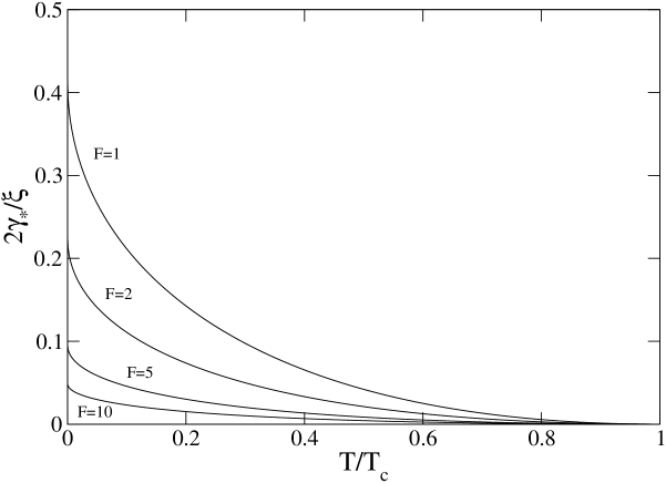
Figure 6: Maximum growth rate as a function of the temperature for different values of the friction parameter $F$.

For $T=T_{c}$, we have

(64) $$k_{J}=k_{0},\qquad k_{m}=0,\qquad k_{d}=k_{0}\sqrt{F},$$

(65) $$2k_{c}^{2}/k_{0}^{2}=F+\sqrt{F^{2}+4F},\qquad 2k_{s}^{2}/k_{0}^{2}=-F+\sqrt{F^{2}+4F},$$

(66) $${2\over\xi}\omega=\sqrt{{k^{4}\over k_{0}^{2}F(k^{2}+k_{0}^{2})}-1},\quad\gamma=-{\xi\over 2},\quad(k>k_{c}),$$

(67) $${2\over\xi}\gamma=-1+\sqrt{1-{k^{4}\over k_{0}^{2}F(k^{2}+k_{0}^{2})}},\quad(k<k_{c}).$$

The system is stable for all wavelengths. The wavenumber marking the appearance of oscillations is $k_{c}(F)$. It behaves like $k_{c}/k_{0}\sim F^{1/4}$ for $F\rightarrow 0$ and $k_{c}/k_{0}\sim F^{1/2}$ for $F\rightarrow+\infty$.

For $T=0$, we find that $k_{m}\rightarrow+\infty$ so that the system is always unstable. The growth rate of the perturbation is given by

(68) $${2\gamma\over\xi}=-1+\sqrt{1+{k^{2}\over F(k_{0}^{2}+k^{2})}}.$$

It increases and tends asymptotically to its maximum value

(69) $${2\gamma_{*}\over\xi}=-1+\sqrt{1+{1\over F}}.$$

For $T>T_{c}$, the system is always stable ($k_{m}^{2}<0$). For $k>k_{c}$, the perturbation undergoes damped oscillations with pulsation (51) and decay rate $\gamma=-{\xi}/{2}$. For $k<k_{c}$, the perturbation decays exponentially with rate (53) tending to $\gamma=0$ for $k=0$. For $T\rightarrow+\infty$ and $F$ finite,

(70) $$k_{J}=0,\qquad k_{m}^{2}/k_{0}^{2}=-1,\qquad k_{d}=0,\qquad k_{c}=0,\qquad k_{s}=k_{0}.$$

The perturbation oscillates with a pulsation $\omega=\sqrt{T}k$, and is damped with a rate $\gamma=-\xi/2$. The case $F\rightarrow+\infty$ is treated in Sec. 3.2.

3.1 The case $\xi=0$

For $\xi=0$ (Euler) and $T\leq T_{c}$, we have

(71) $$k_{m}(T)=k_{c}(T)=k_{0}\left({T_{c}\over T}-1\right)^{1/2},\qquad k_{d}=k_{s}=0.$$

For $k<k_{m}$, the system is unstable and the growth rate is

(72) $$\gamma=\sqrt{T}\left[{k^{2}(k_{m}^{2}-k^{2})\over k^{2}+k_{0}^{2}}\right]^{1/2}.$$

It is maximum for

(73) $$k_{*}(T)/k_{0}=\left[\left({T_{c}\over T}\right)^{1/2}-1\right]^{1/2},$$

with value

(74) $$\gamma_{*}(T)=k_{0}\sqrt{T_{c}}\left[1-\left({T\over T_{c}}\right)^{1/2}\right].$$

For $k>k_{m}$, the system is stable and the perturbation undergoes oscillations with pulsation

(75) $$\omega=\sqrt{T}\left[{k^{2}(k^{2}-k_{m}^{2})\over k^{2}+k_{0}^{2}}\right]^{1/2}.$$

These results are summarized in Fig. 7. For $T=T_{c}$, $k_{m}=0$. The system is always stable and the pulsation is

(76) $$\omega=\sqrt{T_{c}}{k^{2}\over\sqrt{k^{2}+k_{0}^{2}}}.$$

For $T=0$, $k_{m}\sim k_{0}(T_{c}/T)^{1/2}\rightarrow+\infty$. The system is always unstable and the growth rate is

(77) $$\gamma=\sqrt{T_{c}}{k_{0}k\over\sqrt{k^{2}+k_{0}^{2}}}.$$

It increases and tends, for $k\rightarrow+\infty$, to its maximum value $\gamma_{*}=\sqrt{T_{c}}k_{0}=\sqrt{\lambda\overline{\rho}}$. For $\xi=0$ and $T>T_{c}$, we have

(78) $$k_{s}^{2}=-k_{m}^{2}=k_{0}^{2}\left(1-{T_{c}\over T}\right),\qquad k_{d}=k_{c}=0.$$

The system is always stable and the pulsation is

(79) $$\omega=\sqrt{T}\left[{k^{2}(k^{2}+k_{s}^{2})\over k^{2}+k_{0}^{2}}\right]^{1/2}.$$

For $T\rightarrow+\infty$, $k_{s}\rightarrow k_{0}$ and $\omega\sim\sqrt{T}k$.

Figure 7: Growth rate and pulsation as a function of the wavenumber for $\xi=0$. We have taken $T/T_{c}=1/2$, $\lambda\overline{\rho}=1$, $k_{0}=1$.

3.2 The case $\xi\rightarrow+\infty$

For $\xi\rightarrow+\infty$ (Smoluchowski) and $T\leq T_{c}$, we have

(80) $$k_{m}(T)=k_{0}\left({T_{c}\over T}-1\right)^{1/2},\qquad k_{c}\sim k_{d}\rightarrow+\infty,\qquad k_{s}=0.$$

The rate of the exponential evolution is

(81) $$\gamma={T\over\xi}{k^{2}(k_{m}^{2}-k^{2})\over k^{2}+k_{0}^{2}}.$$

For $k>k_{m}$, the perturbation is damped (stable) and the decay rate behaves like $\gamma\sim-(T/\xi)k^{2}$ for $k\rightarrow+\infty$. For $k<k_{m}$ the perturbation increases (unstable). The growth rate is maximum for

(82) $$k_{*}(T)/k_{0}=\left[\left({T_{c}\over T}\right)^{1/2}-1\right]^{1/2},$$

with value

(83) $$\gamma_{*}(T)={k_{0}^{2}T_{c}\over\xi}\left[1-\left({T\over T_{c}}\right)^{1/2}\right]^{2}.$$

These results are summarized in Fig. 8.

Figure 8: Growth rate as a function of the wavenumber for $\xi\rightarrow+\infty$. We have taken $T/T_{c}=1/2$, $\lambda\overline{\rho}=1$, $k_{0}=1$.

For $T=T_{c}$, $k_{m}=0$. The system is always stable and the perturbation decreases with a decay rate

(84) $$\gamma=-{T_{c}\over\xi}{k^{4}\over k^{2}+k_{0}^{2}}.$$

For $T=0$, $k_{m}\rightarrow+\infty$. The system is always unstable and the growth rate is

(85) $$\gamma={k_{0}^{2}T_{c}\over\xi}{k^{2}\over{k^{2}+k_{0}^{2}}}.$$

It increases and tends, for $k\rightarrow+\infty$, to its maximum value $\gamma_{*}={k_{0}^{2}T_{c}/\xi}={\lambda\overline{\rho}/\xi}$. For $\xi\rightarrow+\infty$ and $T>T_{c}$, we have

(86) $$k_{m}^{2}=k_{0}^{2}\left({T_{c}\over T}-1\right)<0,\qquad k_{c}\sim k_{d}\rightarrow+\infty,\qquad k_{s}=0.$$

The system is always stable and the decay rate is

(87) $$\gamma={T\over\xi}{k^{2}(k_{m}^{2}-k^{2})\over k^{2}+k_{0}^{2}}<0.$$

For $T\rightarrow+\infty$, $k_{m}^{2}\rightarrow-k_{0}^{2}$ and $\gamma=-{T\over\xi}k^{2}$.

4 Particular equations of state

The hydrodynamic equations (1)-(3) or the generalized Keller-Segel model (4)-(5) incorporate a pressure force $-\nabla p(\rho)$ associated with a barotropic equation of state $p(\rho)$. At equilibrium, the system satisfies a relation of the form

(88) $$\nabla p=\rho\nabla c.$$

This corresponds to a condition of hydrostatic balance between the pressure force and the chemotactic attraction. For inhomogeneous systems at equilibrium, the density is a function $\rho=\rho(c)$ of the concentration of the chemical obtained by integrating Eq. (88). We have the identities

(89) $$\int^{\rho}\frac{p^{\prime}(x)}{x}dx=c,\qquad\frac{p^{\prime}(\rho)}{\rho}=\frac{1}{\rho^{\prime}(c)},\qquad p^{\prime}(c)=\rho.$$

Since $p^{\prime}(\rho)>0$ in ordinary circumstances, this implies that the density is an increasing function of the concentration of the chemical, i.e. $\rho^{\prime}(c)>0$. On the other hand, for homogeneous systems, the condition of stability (13) can be written

(90) $$\frac{p^{\prime}(\overline{\rho})}{\overline{\rho}}\geq\frac{\lambda}{k_{0}^{2}}.$$

This relation determines the range of densities $\overline{\rho}$ for which the system is stable, depending on the form of the equation of state $p(\rho)$. In particular, the system is stable whatever the value of the density if $\min_{\rho}[{p^{\prime}(\rho)}/{\rho}]\geq\lambda/k_{0}^{2}$ and unstable (for sufficiently large wavelengths) whatever the value of the density if $\max_{\rho}[{p^{\prime}(\rho)}/{\rho}]\leq\lambda/k_{0}^{2}$. The pressure force in Eq. (2) can take into account different effects such as anomalous diffusion or close packing effects. Typically, three kinds of pressure law $p(\rho)$ have been considered in the chemotactic literature:

(i) In the standard case, the pressure is a linear function of the density

(91) $$p=\rho T.$$

This is similar to an isothermal equation of state where $T$ is an effective temperature [14]. When this law is substituted in the drift-diffusion equation (4) we recover the standard Keller-Segel model [3]:

(92) $${\partial\rho\over\partial t}=\nabla\cdot\left(D\nabla\rho-\chi\rho\nabla c\right),$$

where we have introduced the diffusion coefficient $D$ through the Einstein relation $D=\chi T$. The equilibrium state is the Boltzmann distribution $\rho=Ae^{\beta c}$. For the pressure law (91), the velocity of sound has the constant value $c_{s}^{2}=T$. Therefore, the stability criterion (13) can be rewritten in the form

(93) $$T\geq T_{c}\equiv\frac{\lambda\overline{\rho}}{k_{0}^{2}}.$$

For a fixed density $\overline{\rho}$, it defines a critical temperature $T_{c}$ below which the system is unstable. Alternatively, for a fixed temperature $T$, the stability criterion (13) can be rewritten in the form

(94) $$\overline{\rho}\leq\overline{\rho}_{crit}\equiv\frac{k_{0}^{2}T}{\lambda}.$$

The system becomes unstable above a certain critical density ${\rho}_{crit}$.

(ii) In [15, 35], we have proposed to take into account anomalous diffusion by using an equation of state of the form

(95) $$p=K\rho^{\gamma}.$$

This is similar to a polytropic equation of state where $K$ plays the role of a polytropic temperature. When this law is substituted in the drift-diffusion equation (4) we obtain the generalized Keller-Segel model studied in [15, 35]:

(96) $${\partial\rho\over\partial t}=\nabla\cdot\left[\chi\left(K\nabla\rho^{\gamma}-\rho\nabla c\right)\right].$$

The equilibrium state is the Tsallis distribution $\rho=[\lambda+(\gamma-1)/(K\gamma)c]^{1/(\gamma-1)}$ [36]. For the pressure law (95), the velocity of sound has the value $c_{s}^{2}=K\gamma\rho^{\gamma-1}$. Therefore, the stability criterion (13) can be rewritten in the form

(97) $$K\geq K_{c}\equiv\frac{\lambda{{\rho}}^{2-\gamma}}{\gamma k_{0}^{2}}.$$

For a fixed density $\overline{\rho}$, it defines a critical polytropic temperature $K_{c}$ below which the system is unstable. Alternatively, for a fixed polytropic temperature $K$, we can express the stability criterion (13) as a function of the density. We need to distinguish three cases (see Figs. 9 and 10): (a) For $\gamma<2$, the stability criterion can be written in the form

(98) $$\overline{\rho}\leq\overline{\rho}_{crit}\equiv\left(\frac{K\gamma k_{0}^{2}}{\lambda}\right)^{\frac{1}{2-\gamma}}.$$

The system becomes unstable above a critical density. (b) For $\gamma>2$, the stability criterion can be written in the form

(99) $$\overline{\rho}\geq\overline{\rho}_{crit}\equiv\left(\frac{\lambda}{K\gamma k_{0}^{2}}\right)^{\frac{1}{\gamma-2}}.$$

The system becomes unstable below a critical density. (c) For $\gamma=2$, the stability criterion can be written in the form

(100) $$K\geq K_{c}\equiv\frac{\lambda}{2k_{0}^{2}}.$$

The instability threshold is independent on the density.

Figure 9: Graphical construction determining the instability threshold (expressed in terms of the density) for a polytropic equation of state with index $\gamma$. The system is stable if $c_{s}^{2}=K\gamma{\rho}^{\gamma-1}\geq\lambda{\rho}/k_{0}^{2}$ and unstable to sufficiently large wavelengths otherwise. We have taken $K=1$ and $\lambda/k_{0}^{2}=1$.

Figure 10: Stability diagram of a spatially uniform polytropic gas with an attractive Yukawa potential of interaction. The curves represent $K_{c}(\rho)$ or $\rho_{crit}(K)$ and separate the stable region (upper region) from the unstable one (lower region). For $\gamma=1$, we recover the isothermal case with $K=T$. We have taken $\lambda/k_{0}^{2}=1$.

Figure 11: Graphical construction determining the instability threshold (expressed in terms of the density) for an equation of state of the form (101) with temperature $T$. The system is stable if $c_{s}^{2}=T/(1-\rho/\sigma_{0})\geq\lambda{\rho}/k_{0}^{2}$ and unstable to sufficiently large wavelengths otherwise. We have taken $\sigma_{0}=1$ and $\lambda/k_{0}^{2}=1$ leading to a critical temperature $T_{*}=1/4$.

Figure 12: Stability diagram of a spatially uniform gas described by the pressure law (101) with an attractive Yukawa potential of interaction. The curve represents $T_{c}(\rho)$ or $\rho_{\pm}(T)$ and separates the stable region from the unstable one. There exists a critical point $T_{*}$ above which the homogeneous phase is always stable whatever the density. Below $T_{*}$, the homogenous phase is stable for $\rho<\rho_{-}$, unstable for $\rho_{-}<\rho<\rho_{+}$ and stable again for $\rho>\rho_{+}$. This corresponds to a reentrant phase. We have taken $\sigma_{0}=1$ and $\lambda/k_{0}^{2}=1$ leading to a critical temperature $T_{*}=1/4$.

(iii) As a result of chemotactic collapse, the standard Keller-Segel model can lead to finite time singularities and Dirac peaks [2, 14, 16]. In reality, these singularities are unphysical because the cells have a finite size and cannot be compressed indefinitely. Therefore, in more realistic models, we expect that the pressure $p(\rho)$ tends to zero for low densities $\rho\rightarrow 0$ and rapidly increases for large densities. This takes into account the fact that cells do not interpenetrate due to their finite size and this prevents overcrowding. In [37], one of us has proposed to take into account volume filling and finite size effects by using an equation of state of the form

(101) $$p=-T\sigma_{0}\ln(1-\rho/\sigma_{0}).$$

For low densities $\rho\rightarrow 0$, we recover the linear equation of state $p=\rho T$ and for high densities, close to the maximum allowable density $\sigma_{0}$, the pressure rapidly increases and diverges when $\rho\rightarrow\sigma_{0}$. If $a$ represents the typical size of the cells, we have $\sigma_{0}\sim 1/a^{d}$ where $d$ is the dimension of space. When this law is substituted in the drift-diffusion equation (4) we obtain the generalized Keller-Segel model studied in [37]:

(102) $${\partial\rho\over\partial t}=\nabla\cdot\left[\chi\left(\frac{T}{1-\rho/\sigma_{0}}\nabla\rho-\rho\nabla c\right)\right].$$

The steady state of this equation is a Fermi-Dirac distribution in physical space $\rho=\sigma_{0}/(1+\lambda e^{-\beta c})$ putting an upper bound on the density: $\rho\leq\sigma_{0}$ . For the pressure law (101), the velocity of sound is $c_{s}^{2}=T/(1-{\rho}/\sigma_{0})$. Therefore, the stability criterion (13) can be rewritten in the form

(103) $$T\geq T_{c}\equiv\frac{\lambda\overline{\rho}(1-\overline{\rho}/\sigma_{0})}{k_{0}^{2}}.$$

For a fixed density $\overline{\rho}$, it defines a critical temperature $T_{c}$ below which the system is unstable. Alternatively, for a fixed temperature $T$, we can express the stability criterion (13) as a function of the density. The system is stable if

(104) $$\overline{\rho}^{2}-\sigma_{0}\overline{\rho}+\frac{T\sigma_{0}k_{0}^{2}}{\lambda}\geq 0,$$

and unstable to large wavelengths otherwise. The discriminant of this equation is $\Delta=\sigma_{0}^{2}-4T\sigma_{0}k_{0}^{2}/\lambda$. If $\Delta<0$, corresponding to

(105) $$T>T_{*}\equiv\frac{\lambda\sigma_{0}}{4k_{0}^{2}},$$

the system is stable whatever the value of the density (see Figs. 11 and 12). Alternatively, if $T<T_{*}$, the system is stable for $\overline{\rho}<\overline{\rho}_{-}$ and $\overline{\rho}_{+}<\overline{\rho}<\sigma_{0}$ and unstable for $\overline{\rho}_{-}<\overline{\rho}<\overline{\rho}_{+}$ where

(106) $$\overline{\rho}_{\pm}=\frac{\sigma_{0}}{2}\left(1\pm\sqrt{1-\frac{T}{T_{*}}}\right).$$

For low densities ($\rho\ll\sigma_{0}$), the homogenous phase is stable because the chemotactic attraction is not strong enough to overcome diffusive effects (like for a low density isothermal gas (i)) and for high densities ($\rho\rightarrow\sigma_{0}$), the homogeneous phase is stabilized by pressure effects due to close packing. Other generalized Keller-Segel models of chemotaxis are discussed in [39] in relation with nonlinear mean field Fokker-Planck equations.

5 Conclusion

In this paper, we have studied the chemotactic instability of an infinite and homogeneous distribution of cells whose dynamics is described by the hydrodynamic equations (1)-(3). We have shown the analogy with the classical Jeans instability in astrophysics. This close analogy between two systems of a very different nature (stars and bacteria) is very intriguing and deserves to be developed and emphasized. As is well-known, an infinite and homogeneous distribution of stars is not a stationary state of the gravitational Euler-Poisson system [28]. However, if we make the Jeans swindle (which is made in any textbook of astrophysics), the equations for the linear perturbations are the same as in the biological problem (1)-(3) when $\xi=k_{0}=0$. Therefore, the two systems are really analogous. The main differences between the chemotactic problem and the Jeans problem are due to the presence of (i) a friction force $-\xi{\bf u}$ in the Euler equation (2) and (ii) a shielding length $k_{0}^{-1}$ in the equation (3) determining the potential of interaction (played here by the concentration of the secreted chemical). We have studied the effect of these terms in detail. This leads to a generalization of the Jeans instability analysis. The shielding length determines a critical velocity of sound $(c_{s})_{crit}=({\lambda\overline{\rho}}/{k_{0}^{2}})^{1/2}$, so that the system is always stable if $c_{s}>(c_{s})_{crit}$ and becomes unstable to large wavelengths if $c_{s}<(c_{s})_{crit}$. Therefore, the system experiences a phase transition from a homogeneous distribution to an inhomogeneous distribution when the velocity of sound passes below a critical value $(c_{s})_{crit}$. In the usual Jeans problem, the system is always unstable to large wavelengths since $(c_{s})_{crit}=+\infty$. The condition of instability corresponds to $k\leq k_{J}$ where $k_{J}=(\lambda\overline{\rho}/c_{s}^{2})^{1/2}$ is the Jeans wavenumber. For $k_{0}\neq 0$ and $c_{s}<(c_{s})_{crit}$, the condition of instability is $k\leq k_{m}\equiv\sqrt{k_{J}^{2}-k_{0}^{2}}$. Therefore, the effect of the shielding is to shift the instability to larger wavelengths with respect to the Jeans length. In order to measure the influence of the friction parameter $\xi$, we have introduced a wavenumber $k_{d}=\xi/(2c_{s})$ and a dimensionless number $F=(k_{d}/k_{J})^{2}$. The square root of this number $F^{1/2}\sim\xi t_{D}$ corresponds to the ratio between the dynamical time $t_{D}\sim 1/\sqrt{\overline{\rho}\lambda}$ and the friction time $\xi^{-1}$. For $F=0$, Eq. (2) reduces to the Euler equation describing a purely inertial evolution ($t_{D}\ll\xi^{-1}$) and for $F\rightarrow+\infty$, Eqs. (1)- (2) lead to the generalized Smoluchowski equation (4) describing an overdamped evolution ($\xi^{-1}\ll t_{D}$). We have introduced a wavenumber $k_{c}(F)$ which separates, in the zone of stable wavenumbers ($k>k_{m}$), the case of purely exponential decay ($k_{m}<k<k_{c}$) from the case of damped oscillations ($k>k_{c}$). We have also determined, in the unstable zone ($k<k_{m}$), the wavenumber $k_{*}$ corresponding to the maximum growth rate. In the Newtonian model (no shielding) it is equal to $k_{*}=0$ corresponding to infinite wavelengths. In the Yukawa model, it corresponds to a finite wavelength given by Eq. (60), independent on the friction parameter $\xi$. For $c_{s}\rightarrow(c_{s})_{crit}$, $k_{*}\rightarrow 0$ and for $c_{s}\rightarrow 0$, $k_{*}\rightarrow+\infty$ corresponding to small wavelengths. We have found that the shielding length present in the chemotactic model solves many problems inherent to the Jeans analysis. Indeed, there is no Jeans swindle in the chemotactic problem and the maximum growth rate occurs for a finite wavelength (when $k_{0}\neq 0$) instead of an infinite wavelength (when $k_{0}=0$). Therefore, the mathematical problem of linear dynamical stability is better posed in biology than in astrophysics since it avoids the Jeans swindle.

The linear stability analysis performed in this paper gives the condition of instability (in Sec. 4, we have expressed this condition of instability in terms of the density for different equations of state $p(\rho)$ used in the literature) and describes the early development of the instability. When the condition of instability (14) is fulfilled, the perturbation grows until the system can no longer be described by equilibrium or near equilibrium equations. Therefore, the next step is to study the chemotactic collapse in the nonlinear regime to see the formation of patterns like clusters and filaments. A large number of studies in applied mathematics (see the extensive list of references given in the review [2]) and physics [14, 15, 16, 37] have considered the overdamped limit of the model (1)-(3) leading to the Keller-Segel model (4)-(5), similar to the Smoluchowski-Poisson system (9)-(10). For this parabolic model, chemotactic collapse leads to the formation of round clusters. The evolution of an individual cluster in the nonlinear regime can be studied by considering spherically symmetric solutions of the Keller-Segel model. The standard Keller-Segel model (92) leads to the formation of Dirac peaks (for $d\geq 2$) [2, 14, 16]. In the regularized model (102), the Dirac peaks are replaced by smooth aggregates [38, 37]. These aggregates interact with each other and lead to a coarsening process where the number of clusters $N(t)$ decays with time as they collapse to each other. This process may share some analogies with the aggregation of vortices in two-dimensional turbulence [40]. We expect that the decay of the number of clusters depends on the effective range of interaction mediated by the chemical $k_{0}^{-1}$ (shielding length). If the shielding length is small the clusters do not “see” each other and the decay of $N(t)$ should be slowed down or even stopped. In that case, we obtain a quasi stationary state made of clusters separated from each other by a distance of the order of the shielding length $k_{0}^{-1}$. If we take into account inertial effects, using the hyperbolic model (1)-(3) instead of the parabolic model (4)-(5), the collection of isolated clusters is replaced by a network pattern with nodes (clusters) separated by chords [21, 22, 23]. The filaments between two nodes have a length of the order of $k_{0}^{-1}$. Again, the number of nodes should decay with time. However, if the shielding length $k_{0}^{-1}$ is small, the evolution is slowed down and we get a quasi equilibrium state with a filamentary structure corresponding to the initiation of a vasculature [21].

References

- [1] J.D. Murray, Mathematical Biology (Springer, Berlin, 1991).
- [2] D. Horstmann, From 1970 until present: the Keller-Segel model in chemotaxis and its consequences, Jahresber. Deutsch. Math. Verein. 106, 51 (2004).
- [3] E. Keller, L.A. Segel J. theor. Biol. 26, 399 (1970).
- [4] V. Nanjundiah, J. Theoret. Biol. 42, 63 (1973).
- [5] S. Childress, J.K. Percus, Math. Biosci. 56, 217 (1981).
- [6] W. Jäger, S. Luckhaus, Trans. Amer. Math. Soc. 329, 819 (1992).
- [7] T. Nagai, Adv. Math. Sci. Appl. 5, 581 (1995).
- [8] M.A. Herrero, J.L. Velazquez, Math. Ann. 306, 583 (1996).
- [9] H.G. Othmer, A. Stevens, SIAM J. Appl. Math. 57, 1044 (1997).
- [10] M.A. Herrero, E. Medina, J.L. Velazquez, Nonlinearity 10, 1739 (1997).
- [11] M.A. Herrero, E. Medina, J.L. Velazquez, J. Comput. Appl. Math. 97, 99 (1998).
- [12] P. Biler, Adv. Math. Sci. Appl. 8, 715 (1998).
- [13] M.P. Brenner, P. Constantin, L.P. Kadanoff, A. Schenkel, S.C. Venkataramani, Nonlinearity 12, 1071 (1999).
- [14] C. Sire, P.H. Chavanis, Phys. Rev. E 66, 046133 (2002).
- [15] P.H. Chavanis, C. Sire, Phys. Rev. E 69, 016116 (2004).
- [16] C. Sire, P.H. Chavanis, Phys. Rev. E 69, 066109 (2004).
- [17] J. Dolbeault, B. Perthame, C. R. Acad. Sci. Paris, Ser. I 339, 611 (2004).
- [18] P. Biler, G. Karch, P. Laurençot, T. Nadzieja, Topol. Methods Nonlinear Anal. 27, 133 (2006).
- [19] P. Biler, G. Karch, P. Laurençot, T. Nadzieja, Math. Methods Appl. Sci. 29, 1563 (2006).
- [20] P. Carmeliet, Nature Medicine 6, 389 (2000).
- [21] A. Gamba, D. Ambrosi, A. Coniglio, A. de Candia, S. di Talia, E. Giraudo, G. Serini, L. Preziosi, F.A. Bussolino, Phys. Rev. Lett. 90, 118101 (2003).
- [22] F. Filbet, P. Laurençot, B. Perthame, J. Math. Biol. 50, 189 (2005).
- [23] P.H. Chavanis, C. Sire, Physica A 384, 199 (2007) .
- [24] A.J. Chaplain, Math. Comput. Modelling 23, 47 (1996).
- [25] J. Peebles, Large-Scale Structures of the Universe (Princeton University Press, 1980).
- [26] M. Vergassola, B. Dubrulle, U. Frisch, A. Noullez, Astron. Astrophys. 289, 325 (1994).
- [27] P.H. Chavanis, C. Sire, Phys. Rev. E 73, 066104 (2006).
- [28] J. Binney, S. Tremaine, Galactic Dynamics (Princeton Series in Astrophysics, 1987).
- [29] P.H. Chavanis, Phys. Rev. E 68, 036108 (2003).
- [30] P.H. Chavanis, Banach Center Publ. 66, 79 (2004).
- [31] A. Alastuey, Ann. Phys. Fr. 11, 653 (1986).
- [32] P.H. Chavanis, Astron. Astrophys. 381, 340 (2002).
- [33] A. Pais, “Subtle is the Lord…” The Science and the Life of Albert Einstein (Oxford University Press, 1982).
- [34] P.H. Chavanis, Eur. Phys. J. B 52, 433 (2006).
- [35] P.H. Chavanis, C. Sire, Physica A 387, 1999 (2008).
- [36] C. Tsallis, J. Stat. Phys. 52, 479 (1988).
- [37] P.H. Chavanis, Eur. Phys. J. B 54, 525 (2006).
- [38] T. Hillen, K. Painter, Adv. Appl. Math. 26, 280 (2001).
- [39] P.H. Chavanis, [arXiv:0709.1829]
- [40] C. Sire, P.H. Chavanis, Phys. Rev. E 61, 6644 (2000).