Power-law expansion cosmology in Schrödinger-type formulation

Abstract

We investigate non-linear Schrödinger-type formulation of cosmology of which our cosmological system is a general relativistic FRLW universe containing canonical scalar field under arbitrary potential and a barotropic fluid with arbitrary spatial curvatures. We extend the formulation to include phantom field case and we have found that Schrödinger wave function in this formulation is generally non-normalizable. Assuming power-law expansion, $a\sim t^{q}$, we obtain scalar field potential as function of time. The corresponding quantities in Schrödinger-type formulation such as Schrödinger total energy, Schrödinger potential and wave function are also presented.

I Introduction

Canonical scalar field plays important role in inflationary phase in the early universe as well as acceleration in the late universe observed and confirmed by cosmic microwave background Masi:2002hp , large scale structure surveys Scranton:2003in and supernovae type Ia Riess:1998cb . The scalar field is considered as inflaton field in inflationary models inflation . It could also be considered as dark energy that drives the late acceleration described in review literatures Padmanabhan:2004av and references therein. In standard cosmology with Friedmann-Lemaître-Robertson-Walker (FLRW) background, major components of the late universe are mixture of dark matter which is a type of barotropic fliud and dark energy in form of scalar field. When assuming pure scalar fluid in flat universe, one can obtain analytical solutions otherwise the problem can also be solved numerically. However, considering arbitrary types of barotropic fluid and a non-flat universe, it is not always possible to solve the system analytically.

Apart from standard cosmological equations, there are few alternative mathematical formulations which are also equivalent to the scalar field cosmology with barotropic fluid. One is in form of non-linear Ermakov-attemping equation Hawkins:2001zx and another idea proposed recently is in form of non-Ermakov-Milne-Pinney (non-EMP) equation. Cosmological equations in the latter proposal can be written in form of a non-linear Schrödinger-type equation when imposing relations between quantities in standard cosmological equations and Schrödinger-type equation D'Ambroise:2006kg . In case of Bianchi I scalar field cosmology, recent work shows that it is possible to construct a corresponding linear Schrödinger-type equation by redefining cosmological quantities D'Ambroise:2007gm . With the new representation, scalar field cosmology is reinterpreted in new way which might be able to give new methods of approaching mathematical problems in scalar field cosmology.

There are various observations allowing scalar field equation of state coefficient, $w_{\phi}$ to be less than -1 Melchiorri:2002ux . Recent data such as a combined WMAP, LSS and SN type Ia without assuming flat universe, puts a strong constraint, $w_{\phi}=-1.06^{+0.13}_{-0.08}$ Spergel:2006hy . Also the first result from ESSENCE Supernova Survey Ia combined with SuperNova Legacy Survey Ia assuming flat universe, gives a constraint of $w_{\phi}=-1.07\pm 0.09$ Wood-Vasey:2007jb . Therefore it is possible that the scalar field dark energy could be phantom, i.e $w_{\phi}<-1$ Caldwell:1999ew . The phantom behavior, $w_{\phi}<-1$ can be attained by negative kinetic energy term of the scalar field density and pressure. In FLRW standard cosmology, the field can yield big rip singularity, i.e. $a,\rho,|p|\rightarrow\infty$ at finite time Caldwell:2003vq with attempts of singularity avoidance in several ways Sami:2005zc .

In this work, we investigate connection between standard cosmological equations and non-linear Schrödinger-type equation with a comment on normalization of the wave function. We modify the work of D'Ambroise:2006kg to include phantom field case. A case of power-law expansion with scalar field and dark matter is considered as a toy model. We begin from Sec. II where we introduce our cosmological system. Afterward in Sec. III, we discuss how non-linear Schrödinger-type formulation quantities are related to quantities in standard scalar field cosmology. In non-linear Schrödinger-type equation, one important quantity is wave function. We comment on normalization properties of the wave function in Sec. IV. We consider a case of power-law expansion in Sec. V before deriving scalar field potential, Schrödinger potential and Schrödinger wave function. At last we conclude this work in Sec. VI.

II Cosmological equations

In a Friedmann-Lemaître-Robertson-Walker universe, the Einstein field equations are

$$H^{2} = \frac{\kappa^{2}\rho_{\rm t}}{3}-\frac{k}{a^{2}}\,,$$ (1)

$$\frac{\ddot{a}}{a} = -\frac{\kappa^{2}}{6}(\rho_{\rm t}+3p_{\rm t})\,,$$ (2)

where $\kappa^{2}\equiv 8\pi G=1/M_{\rm P}^{2}$, $G$ is Newton’s gravitational constant, $M_{\rm P}$ is reduced Planck mass, $k$ is spatial curvature, $\rho_{\rm t}$ and $p_{\rm t}$ are total density and total pressure, i.e. $\rho_{\rm t}=\rho_{\gamma}+\rho_{\phi}$ and $p_{\rm t}=p_{\gamma}+p_{\phi}$. The barotropic component is denoted by $\gamma$, while for scalar field, by $\phi$. Equations of state for barotropic fluid and scalar field are $p_{\gamma}=w_{\gamma}\rho_{\gamma}$ and $p_{\phi}=w_{\phi}\rho_{\phi}$. We consider minimally couple scalar field with Lagrangian density,

$$\mathcal{L}=\frac{1}{2}\epsilon\dot{\phi}^{2}-V(\phi)\,,$$ (3)

where $\epsilon=1$ for non-phantom case and $-1$ for phantom case. Density and pressure of the field are given as

$$\rho_{\phi} = \frac{1}{2}\epsilon\dot{\phi}^{2}+V(\phi)\,,$$ (4)

$$p_{\phi} = \frac{1}{2}\epsilon\dot{\phi}^{2}-V(\phi)\,,$$ (5)

therefore

$$w_{\phi}=\frac{\epsilon\dot{\phi}^{2}-2V(\phi)}{\epsilon\dot{\phi}^{2}+2V(\phi)}\,.$$ (6)

The field obeys conservation equation

$$\epsilon\left[\ddot{\phi}+3H\dot{\phi}\right]+\frac{{\rm d}V}{{\rm d}\phi}=0\,.$$ (7)

For the barotropic fluid, we set $w_{\gamma}\equiv(n-3)/3$ so that $n=3(1+w_{\gamma})$. Hence for cosmological constant $n=0$, for fluid at acceleration bound ($w_{\gamma}=-1/3$) $n=2$, for dust $n=3$, for radiation $n=4$, and for stiff fluid $n=6$. Solution of conservation equation for a barotropic fluid can be obtained directly by solving the conservation equation. The solution is

$$\rho_{\gamma}=\frac{D}{a^{3(1+w_{\gamma})}}=\frac{D}{a^{n}}\,,$$ (8)

then

$$p_{\gamma}=w_{\gamma}\frac{D}{a^{n}}=\frac{(n-3)}{3}\frac{D}{a^{n}}\,,$$ (9)

where a proportional constant $D\geq 0$. Using Eqs. (1), (4), (5), (7) and (8), it is straightforward to show that

$$\epsilon\dot{\phi}(t)^{2} = -\frac{2}{\kappa^{2}}\left[\dot{H}-\frac{k}{a^{2}}\right]-\frac{nD}{3a^{n}}\,,$$ (10)

$$V(\phi) = \frac{3}{\kappa^{2}}\left[H^{2}+\frac{\dot{H}}{3}+\frac{2k}{3a^{2}}\right]+\left(\frac{n-6}{6}\right)\frac{D}{a^{n}}\,.$$ (11)

Therefore if one knows how the scale factor evolves with time, the scalar field velocity and potential can always be expressed as a function of time explicitly.

III Non-linear Schrödinger-type equation

Non-linear Schrödinger-type equation corresponding to canonical scalar field cosmology with barotropic fluid is given by D'Ambroise:2006kg

$$\frac{{\rm d}^{2}}{{\rm d}x^{2}}u(x)+\left[E-P(x)\right]u(x)=-\frac{nk}{2}u(x)^{(4-n)/n}\,.$$ (12)

Quantities in the Schrödinger-type equation above, e.g. wave function $u(x)$, total energy $E$ and Schrödinger potential $P(x)$ are related to the standard cosmology quantities as

$$u(x) \equiv a(t)^{-n/2}\,,$$ (13)

$$E \equiv -\frac{\kappa^{2}n^{2}}{12}D\,,$$ (14)

$$P(x) \equiv \frac{\kappa^{2}n}{4}a(t)^{n}\epsilon\dot{\phi}(t)^{2}\,.$$ (15)

The mapping from cosmic time $t$ to the variable $x$ is via

$$x=\sigma(t),$$ (16)

such that

$$\dot{\sigma}(t) = u(x)\,,$$ (17)

$$\phi(t) = \psi(x)\,.$$ (18)

We notice that relation

$$\psi^{\prime}(x)^{2}=\frac{4}{\kappa^{2}n}P(x)$$ (19)

in Ref. D'Ambroise:2006kg which gives $\psi(x)=\pm({2}/{\kappa\sqrt{n}})\int{\sqrt{P(x)}}\,{\rm d}x\,$ does not include phantom field case. In order to include the phantom field case, we modify relation $\dot{\phi}(t)=\dot{x}\,\psi^{\prime}(x)$ in D'Ambroise:2006kg to $\epsilon\dot{\phi}(t)^{2}=\dot{x}^{2}\,\epsilon\,\psi^{\prime}(x)^{2}$ of which the field kinetic term ($\dot{\phi}^{2}$) is considered instead of the field velocity ($\dot{\phi}$) so that the parameter $\epsilon$ can be included. Therefore, to include the phantom field case, corrected relation to Eq. (19) is

$$\epsilon\,\psi^{\prime}(x)^{2}=\frac{4}{\kappa^{2}n}\,P(x)\,,$$ (20)

and $\psi(x)$ should read

$$\psi(x)=\pm\frac{2}{\kappa\sqrt{n}}\int{\sqrt{\frac{P(x)}{\epsilon}}}\,{\rm d}x\,\,.$$ (21)

Inverse function of $\psi(x)$ exists if $P(x)\neq 0$ and $n\neq 0$. It is important for $\psi^{-1}(x)$ to exist as a function since existence of the relation $x=\sigma(t)$ (Eq. (16)) needs a condition,

$$x=\psi^{-1}\circ\phi(t)=\sigma(t)\,.$$ (22)

In case that $P(x)=0$ and $n\neq 0$, then $\psi=C$, hence inverse of $\psi$ is not a function since one $x$ gives infinite values of $\psi^{-1}$. In this case the relation (22) is invalid. If the inverse function, $\psi^{-1}$ exists (i.e. $P(x)\neq 0$ and $n\neq 0$), then the scalar field potential, $V\circ\sigma^{-1}(x)$ can be expressed as a function of time,

$$V(t)=\frac{12}{\kappa^{2}n^{2}}\left(\frac{{\rm d}u}{{\rm d}x}\right)^{2}-\frac{2u^{2}}{\kappa^{2}n}P(x)+\frac{12u^{2}}{\kappa^{2}n^{2}}E+\frac{3ku^{4/n}}{\kappa^{2}}\,.$$ (23)

Although the potential obtained is not expressed as function of $\phi$, however if one can integrate Eq. (10) to obtain $\phi(t)$, the obtained solution can be inserted into a known function $V(\phi)$ motivated from fundamental physics. Then one can check which fundamental theories give a matched potential to $V(t)$. The Eqs. (11) and (23) are indeed equivalent. Both require only the knowledge of $a(t)$, $D$ and $k$ which can be constrained by observation. Therefore $V(t)$ in both Eqs. (11) and (23) can be constructed if knowing these observed parameters. To construct $V(t)$ in Eq. (23), one needs to know $a(t)$ as a function of time in order to find $u(x)$ and $P(x)$. However, in constructing $V(t)$ in Eq. (11), if knowing $a(t),D$ and $k$, one can directly use these quantities without employing Schrödinger-type quantities.

IV Normalization condition of wave function

Normalization condition for a wave function $u(x)$ in quantum mechanics is

$$\int_{-\infty}^{\infty}|u(x)|^{2}{\rm d}x=1\,.$$ (24)

The wave function here expressed as $u(x)\equiv a^{-n/2}=\dot{x}(t)$, when applying to the normalization condition, reads

$$\int_{-\infty}^{\infty}\dot{x}^{2}{\rm d}x=1\,.$$ (25)

In order to satisfy the condition, $x$ must be constant and so is $t$. Since the form of the wave function must be $u(x)=\dot{x}(t)$ in order to connect equations of cosmology to the Schrödinger-type formulation, therefore $u(x)$ as defined is, in general, non-normalizable.

V Power-law expansion

Here in this section, we apply the method above to the power-law expansion in scalar field cosmology with barotropic fluid in a non-flat universe. The power-law expansion of the universe during inflation era,

$$a(t)=t^{q}\,,$$ (26)

with $q>1$ was proposed by Lucchin and Matarrese Lucchin to give exponential potential

$$V(\phi)=\left[\frac{q(3q-1)}{\kappa^{2}t_{0}^{2}}\right]\exp\left\{-\kappa\sqrt{\frac{2}{q}}\left[\phi(t)-\phi(t_{0})\right]\right\}\,,$$ (27)

assuming domination of scalar field, negligible radiation density and negligible spatial curvature. Recent results from X-Ray gas of galaxy clusters put a constraint of $q\sim 2.3$ for $k=0$, $q\sim 1.14$ for $k=-1$ and $q\sim 0.95$ for $k=1$ Zhu:2007tm . Considering mixture of both fluids, we use effective equation of state, $w_{\rm eff}=({\rho_{\phi}w_{\phi}+\rho_{\gamma}w_{\gamma}})/{\rho_{\rm t}}.$ For a flat universe, the power law expansion, $a=t^{q}$, is attained when $-1<w_{\rm eff}<-1/3$ where $q=2/[3(1+w_{\rm eff})]$. If using $q=2.3$ as mentioned above, it gives $w_{\rm eff}=-0.71$.

V.1 Relating Schrödinger quantities to standard cosmological quantities

Assuming power-law expansion and using Eqs. (13) and (17), Schrödinger wave function is related to standard cosmological quantity as

$$u(x)=\dot{\sigma}(t)=t^{-qn/2}\,.$$ (28)

We can integrate the equation above so that the Schrödinger scale, $x$ is related to cosmic time scale, $t$ as

$$x=\sigma(t)=-\frac{t^{-\beta}}{\beta}+\tau\,,$$ (29)

where $\beta\equiv(qn-2)/2$ and $\tau$ is an integrating constant. The parameters $x$ and $t$ have the same dimension since $\beta$ is only a number. Using Eq. (26), we can find $\epsilon\dot{\phi}(t)^{2}$ from Eq. (10):

$$\epsilon\dot{\phi}(t)^{2}=\frac{2q}{\kappa^{2}t^{2}}+\frac{2k}{\kappa^{2}t^{2q}}-\frac{nD}{3t^{qn}}\,.$$ (30)

We use Eqs. (26) and (30) in Eq. (15), therefore the Schrödinger potential is found to be

$$P(x)=\frac{qn}{2}t^{qn-2}+\frac{kn}{2}t^{q(n-2)}-\frac{\kappa^{2}n^{2}D}{12}\,.$$ (31)

With $E=-\kappa^{2}n^{2}D/12$, the Schrödinger kinetic energy is

$$T=-\frac{qn}{2}t^{qn-2}-\frac{kn}{2}t^{q(n-2)}\,.$$ (32)

V.2 Scalar field potential $V(t)$

In order to obtain $V(t)$ in Eq. (23), we need to know derivative of $u(x)$:

$$\frac{{\rm d}}{{\rm d}x}\,u(x) = -\frac{qn}{2t}\,.$$ (33)

At this step, using Eqs. (13), (14), (15) and (33) in Eq. (23), we finally obtain

$$V(t)=\frac{q(3q-1)}{\kappa^{2}t^{2}}+\frac{2k}{\kappa^{2}t^{2q}}+\left(\frac{n-6}{6}\right)\frac{D}{t^{qn}}\,.$$ (34)

Assuming flat universe ($k=0$) and $q=2.3$, we show $V(t)$ in Fig. 1. Thickest line on top is of the case scalar field without barotropic fluid. The middle line is the case when the dust is presented with scalar field ($D\neq 0,n=3$). The bottom line is the case of radiation ($D\neq 0,n=4$). The $V(t)$ plots from the Schrödinger-type formulation matches the plots from standard cosmological equations. The result is independent of $\epsilon$ values. The solution $\phi(t)$ of Eq. (30) can not be integrated if $\epsilon=-1$ or if the integrand of Eq. (30) is imaginary. When $\epsilon=1$ with dust ($D\neq 0,n=3$) and $q=2.3$, the integrand is imaginary. We therefore assume $q=2$ to show numerical integrations in Fig. 2 for the case $D=0,k=0$ and the case $D\neq 0,n=3,k=0$. In the pure scalar field case $D=0,k=0$, numerical solution matches the analytical solution $\phi(t)=(\sqrt{2q}/\kappa)\ln(t)$. This solution can be substituted into Eq. (34) to obtain Eq. (27) as in Lucchin (setting $t_{0}=1$ and $\phi(t_{0})=0$). When considering cases of closed, flat and open universe containing dust matter, $V(t)$ of each case is presented in Fig. 3 where $q=2$ is assumed in all cases so that we can see how the plots change their shapes when $k$ is varied. It is worth noting that reconstruction of scalar field potential assuming scaling solution was considered before in Rubano:2001 .

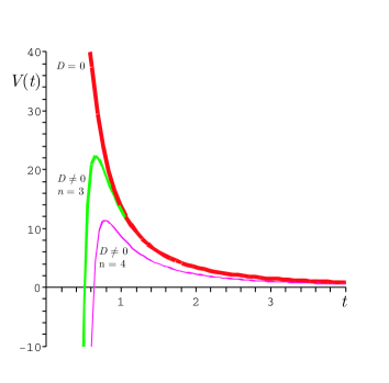
Figure 1: Potential $V(t)$ plots from non-linear Schrödinger-type formulation assuming $a\sim t^{q}$, $q=2.3$ in flat universe ($k=0$). The thickest line is when there is no barotropic fluid $D=0$. The middle line is when there is dust fluid together with scalar field, i.e. $D\neq 0$ and $n=3$. The small line is when the universe has scalar field with radiation fluid, i.e. $D\neq 0$ and $n=4$. We set $\kappa=1$ and in the last two plots, we set $D=1$. All plots match results obtained from standard cosmological equations.

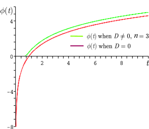
Figure 2: $\phi(t)$ for power-law expansion $a\sim t^{q}$, $q=2$ in flat universe ($k=0$). The red line is of the when the barotropic fluid density is negligible. The green line is in the presence of scalar field with dust ($D\neq 0$ and $n=3$). In the figure, $\kappa=1$ and $D=1$.

V.3 Schrödinger potential $P(x)$

We can find Schrödinger potential $P(x)$ from Eqs. (29) and (31) where time is expressed as a function of $x$ as

$$t(x)=\frac{1}{\left[-\beta(x-\tau)\right]^{1/\beta}}\,.$$ (35)

Therefore

$$P(x) = \frac{2qn}{(qn-2)^{2}}\frac{1}{(x-\tau)^{2}}+\>\frac{kn}{2}\left[\frac{-2}{(qn-2)(x-\tau)}\right]^{2q(n-2)/(qn-2)}-\>\frac{\kappa^{2}n^{2}D}{12}\,.$$ (36)

As in Eq. (32), the Schrödinger kinetic energy is

$$T(x) = -\>\frac{2qn}{(qn-2)^{2}}\frac{1}{(x-\tau)^{2}}-\>\frac{kn}{2}\left[\frac{-2}{(qn-2)(x-\tau)}\right]^{2q(n-2)/(qn-2)}.$$ (37)

The kinetic term has contribution only from the power $q$ and spatial curvature $k$. A disadvantage of Eq. (36) is that we can not use it in the case of scalar field domination as in inflationary era. Dropping $D$ term in Eq. (36) can not be considered as scalar field domination case since the barotropic fluid coefficient $n$ still appears in the other terms. The non-linear Schrödinger-type formulation is therefore suitable when there are both scalar field and a barotropic fluid together such as the situation when dark matter and scalar field dark energy live together in the late universe. The Schrödinger potentials $P(x)$ plotted with $x$ for power-law expansion with $q=2$ in closed, flat and open universe are shown in Fig. 4. In the figure, the dust cases are shown on the right and radiation cases are on the left. We set $\kappa=1,D=1$ and $\tau=0$.

V.4 Schrödinger wave function $u(x)$

The quantity analogous to Schrödinger wave function can be directly found from Eqs. (28) and (35) as

$$u(x)=\left[\left(-\frac{1}{2}qn+1\right)(x-\tau)\right]^{qn/(qn-2)}\,,$$ (38)

which is independent of the spatial curvature $k$ or the initial density $D$. However, coefficient $n$ of the barotropic fluid equation of state and $q$ must be expressed. Wave functions for a range of barotropic fluids are presented in Fig. 5. The result is confirmed by substituting Eq. (38) into Eq. (12).

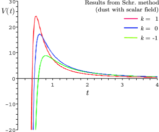
Figure 3: $V(t)$ obtained from non-linear Schrödinger-type formulation for closed, flat and open universe in presence of dust and scalar field.

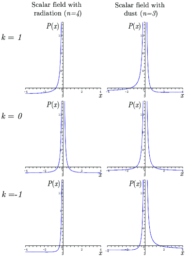
Figure 4: $P(x)$ plotted versus $x$ for power-law expansion. We set $q=2,\kappa=1,D=1$ and $\tau=0$. The scalar field dominant case can not be plotted because even tough we set a condition $D=0$, the coefficient $n$ of the barotropic fluid equation of state still appears in the first and second terms of the Eq. (36). There is only a real-value $P(x)$ for the cases $k=\pm 1$ with $n=4$ because, when $x>0$, $P(x)$ becomes imaginary in these cases.

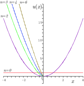
Figure 5: $u(x)$ plotted versus $x$ for power-law expansion with $q=2$. We set $\tau=0$. The wave function is plotted for $n=0$ (cosmological constant), $n=2$, $n=3$ (dust), $n=4$ (radiation) and $n=6$ (stiff fluid). There is no real-value wave function for $n=3$, $n=4$ and $n=6$ unless $x<0$.

VI Conclusions and Comments

We consider Schrödinger-type formulation for a system of canonical scalar field and a barotropic fluid in standard FLRW cosmology with zero or non-zero spatial curvature. In the Schrödinger-type formulation, all quantities in cosmology are represented in Schrödinger-like quantities and the equation relating these Schrödinger-like quantities is written as a non-linear Schrödinger-type equation. If $a(t)$ is known as an exact function of time, a connection of two scale quantities, $x$ and $t$ can be found and then other Schrödinger-like quantities can be determined. We modified the formulation to include the phantom field case. The equation can be simplified to linear type if we consider the flat universe case $k=0$ or the cases $n=2$ or $n=4$ D'Ambroise:2006kg . However, even if the equation is linear, it can not be considered as an analog to non-relativistic time-independent quantum mechanics because in this work, the wave function of Schrödinger-type formulation is found to be, in general, non-normalizable. Afterward, we consider a particular case of power-law expansion of scale factor. We show relations between cosmological quantities in conventional form and in Schrödinger-like form for power-law expansion. We obtain scalar field potential $V(t)$, Schrödinger potential $P(x)$ and wave function $u(x)$. In the case of a scalar field dominant in flat universe, our analytical results $V(\phi)$ and $\dot{\phi}$ agree well with the well-known results in Lucchin . A range of plots in various cases of closed, flat or open geometries is presented. Wave functions for the power-law expansion case (seen in the Fig. 5) are found to be all non-normalizable as conjectured.

Without knowledge of $a(t)$, one might wonder if we could start the calculation procedure from solving the Schrödinger-type equation (12) for example, the linear case as done in basic quantum mechanics. However, in order to do this, we must know the Schrödinger potential $P(x)$ (Eq. (15)) which depends explicitly on $a(t)$ and $\dot{\phi}$. Nevertheless, $\dot{\phi}$ (Eq. (10)) also depends on $a(t)$. Therefore we need to know the law of expansion $a(t)$ before proceeding the calculation. Knowing $a(t)$ enables us to know $u(x)$ directly (see Eq. (28)). Hence in Schrödinger-type formulation, we do not work as in basic quantum mechanics in which major task is to solve the Schrödinger equation for $u(x)$. There could be many solutions of a Schrödinger-type equation. In quantum mechanics valid solutions $u(x)$ must be only normalizable type. Here, unlike in quantum mechanics, our $u(x)$ must be non-normalizable.

At late time the scalar field dark energy and cold dark matter (dust) are two major components of the universe while the others are negligible. For power-law expansion, the procedure is suitable for studying the system of scalar field dark energy and dark matter because it gives all real-value of $P(x)$ for any $k$. We need to know $a(t)$, $k$ and $D$ which are observable in order to find $V(t)$. Information of $V(\phi)$ is important because it is a link to fundamental physics. If one starts from fundamental physics with a particular potential $V(\phi)$ and if also knowing how $\phi$ evolves with $t$, then $V$ could be expressed as function of $t$. Finally, the potential $V(t)$ obtained from observation and another $V(t)$ proposed by fundamental physics can be compared. The non-linear Schrödinger-type formulation might provide an alternative mathematical approach to problem solving in scalar field cosmology.

References

- (1) S. Masi et al., Prog. Part. Nucl. Phys. 48, 243 (2002) [arXiv: astro-ph/0201137]; C. L. Bennett et al., Astrophys. J. Suppl. 148, 1 (2003) [arXiv: astro-ph/0302207]; D. N. Spergel et al. [WMAP Collaboration], Astrophys. J. Suppl. 148 (2003) 175 [arXiv: astro-ph/0302209].
- (2) R. Scranton et al. [SDSS Collaboration], [arXiv: astro-ph/0307335].
- (3) A. G. Riess et al. [Supernova Search Team Collaboration], Astron. J. 116, 1009 (1998) [arXiv: astro-ph/9805201]; S. Perlmutter et al. [Supernova Cosmology Project Collaboration], Astrophys. J. 517, 565 (1999) [arXiv: astro-ph/9812133]; A. G. Riess, arXiv: astro-ph/9908237; G. Goldhaber et al. [The Supernova Cosmology Project Collaboration], arXiv: astro-ph/0104382; J. L. Tonry et al. [Supernova Search Team Collaboration], Astrophys. J. 594, 1 (2003) [arXiv: astro-ph/0305008].
- (4) D. Kazanas, Astrophys. J. 241 L59 (1980); A. A. Starobinsky, Phys. Lett. B 91, 99 (1980); A. H. Guth, Phys. Rev. D 23, 347 (1981); K. Sato, Mon. Not. Roy. Astro. Soc. 195, 467 (1981); A. Albrecht and P. J. Steinhardt, Phys. Rev. Lett. 48, 1220 (1982); A. D. Linde, Phys. Lett. B 108, 389 (1982).
- (5) T. Padmanabhan, Curr. Sci. 88, 1057 (2005) [arXiv: astro-ph/0411044]; E. J. Copeland, M. Sami and S. Tsujikawa, Int. J. Mod. Phys. D 15, 1753 (2006) [arXiv: hep-th/0603057]; T. Padmanabhan, AIP Conf. Proc. 861, 179 (2006) [arXiv: astro-ph/0603114].
- (6) R. M. Hawkins and J. E. Lidsey, Phys. Rev. D 66, 023523 (2002) [arXiv: astro-ph/0112139]; F. L. Williams and P. G. Kevrekidis, Class. Quant. Grav. 20, L177 (2003); J. E. Lidsey, Class. Quant. Grav. 21, 777 (2004) [arXiv: gr-qc/0307037]; F. L. Williams, P. G. Kevrekidis, T. Christodoulakis, C. Helias, G. O. Papadopoulos and T. Grammenos, Trends in Gen. Rel. and Quant. Cosmol., Nova Science Pub. 37-48 (2006) [arXiv: gr-qc/0408056]; F. L. Williams, Int. J. Mod. Phys. A 20 (2005) 2481; A. Kamenshchik, M. Luzzi and G. Venturi, arXiv: math-ph/0506017.
- (7) J. D’Ambroise and F. L. Williams, Int. J. Pure Appl. Maths. 34, 117 (2007) [arXiv: hep-th/0609125].
- (8) J. D’Ambroise, Int. J. Pure Appl. Maths. 3, 417 (2008), arXiv:0711.3916 [hep-th].
- (9) A. Melchiorri, L. Mersini-Houghton, C. J. Odman and M. Trodden, Phys. Rev. D 68, 043509 (2003) [arXiv:astro-ph/0211522]; P. S. Corasaniti, M. Kunz, D. Parkinson, E. J. Copeland and B. A. Bassett, Phys. Rev. D 70, 083006 (2004) [arXiv:astro-ph/0406608]; U. Alam, V. Sahni, T. D. Saini and A. A. Starobinsky, Mon. Not. Roy. Astron. Soc. 354, 275 (2004) [arXiv:astro-ph/0311364].
- (10) D. N. Spergel et al., arXiv:astro-ph/0603449.
- (11) W. M. Wood-Vasey et al., arXiv:astro-ph/0701041.
- (12) R. R. Caldwell, Phys. Lett. B 545, 23 (2002) [arXiv:astro-ph/9908168]; G. W. Gibbons, arXiv:hep-th/0302199; S. Nojiri and S. D. Odintsov, Phys. Lett. B 562 (2003) 147 [arXiv:hep-th/0303117].
- (13) R. R. Caldwell, M. Kamionkowski and N. N. Weinberg, Phys. Rev. Lett. 91, 071301 (2003) [arXiv:astro-ph/0302506]; S. Nesseris and L. Perivolaropoulos, Phys. Rev. D 70, 123529 (2004) [arXiv:astro-ph/0410309]; J. g. Hao and X. z. Li, Phys. Rev. D 67, 107303 (2003) [arXiv:gr-qc/0302100]; X. z. Li and J. g. Hao, Phys. Rev. D 69, 107303 (2004) [arXiv:hep-th/0303093]; P. Singh, M. Sami and N. Dadhich, Phys. Rev. D 68, 023522 (2003) [arXiv:hep-th/0305110]; J. G. Hao and X. z. Li, Phys. Rev. D 70, 043529 (2004) [arXiv:astro-ph/0309746]; M. Sami and A. Toporensky, Mod. Phys. Lett. A 19, 1509 (2004) [arXiv:gr-qc/0312009]; S. Nojiri, S. D. Odintsov and S. Tsujikawa, Phys. Rev. D 71 063004 (2005); B. Gumjudpai, T. Naskar, M. Sami and S. Tsujikawa, JCAP 0506, 007 (2005) [arXiv:hep-th/0502191]; L. A. Urena-Lopez, JCAP 0509, 013 (2005) [arXiv:astro-ph/0507350].
- (14) S. Nojiri, S. D. Odintsov and M. Sasaki, Phys. Rev. D 71, 123509 (2005) [arXiv:hep-th/0504052]; M. Sami, A. Toporensky, P. V. Tretjakov and S. Tsujikawa, Phys. Lett. B 619, 193 (2005) [arXiv:hep-th/0504154]; G. Calcagni, S. Tsujikawa and M. Sami, Class. Quant. Grav. 22, 3977 (2005) [arXiv:hep-th/0505193]; H. Wei and R. G. Cai, Phys. Rev. D 72, 123507 (2005) [arXiv:astro-ph/0509328]; B. M. Leith and I. P. Neupane, arXiv:hep-th/0702002; D. Samart and B. Gumjudpai, Phys. Rev. D 76, 043514 (2007) arXiv:0704.3414 [gr-qc]; T. Naskar and J. Ward, Phys. Rev. D 76, 063514 (2007) [arXiv:0704.3606[gr-qc]]; B. Gumjudpai, Thai J. Phys. Series 3: Proc. of the SIAM Phys. Cong. 2007 [arXiv:0706.3467 [gr-qc]].
- (15) F. Lucchin and S. Matarrese, Phys. Rev. D 32, 1316 (1985).
- (16) Z. H. Zhu, M. Hu, J. S. Alcaniz and Y. X. Liu, Astron. and Astrophys. 483, 15 (2008)
- (17) C. Rubano and J. D. Barrow, Phys. Rev. D 64, 127301 (2001).