A large population of mid-infrared selected, obscured
active galaxies in the Boötes field

Abstract

We identify a population of 640 obscured and 839 unobscured AGNs at redshifts $0.7<z\lesssim 3$ using multiwavelength observations of the 9 deg² NOAO Deep Wide-Field Survey (NDWFS) region in Boötes. We select AGNs on the basis of Spitzer IRAC colors obtained by the IRAC Shallow Survey. Redshifts are obtained from optical spectroscopy or photometric redshift estimators. We classify the IR-selected AGNs as IRAGN 1 (unobscured) and IRAGN 2 (obscured) using a simple criterion based on the observed optical to mid-IR color, with a selection boundary of $R-[4.5]=6.1$, where $R$ and [4.5] are the Vega magnitudes in the $R$ and IRAC 4.5 $\mu$m bands, respectively. We verify this selection using X-ray stacking analyses with data from the Chandra XBoötes survey, as well as optical photometry from NDWFS and spectroscopy from MMT/AGES. We show that (1) these sources are indeed AGNs, and (2) the optical/IR color selection separates obscured sources (with average $N_{\rm H}\sim 3\times 10^{22}$ cm^-2 obtained from X-ray hardness ratios, and optical colors and morphologies typical of galaxies) and unobscured sources (with no X-ray absorption, and quasar colors and morphologies), with a reliability of $\gtrsim 80\%$. The observed numbers of IRAGNs are comparable to predictions from previous X-ray, optical, and IR luminosity functions, for the given redshifts and IRAC flux limits. We observe a bimodal distribution in $R-[4.5]$ color, suggesting that luminous IR-selected AGNs have either low or significant dust extinction, which may have implications for models of AGN obscuration.

1. Introduction

In unified models of active galactic nuclei (AGNs), a significant number of objects are expected to be obscured by a torus of gas and dust that surrounds the central engine and blocks the optical emission along some lines of sight (see reviews by Urry & Padovani, 1995; Antonucci, 1993). In addition, some models of merger-driven quasar activity predict a prolonged phase in which the central engine is entirely obscured, followed by a “blowout” of the absorbing material and a relatively short unobscured phase (e.g., Silk & Rees, 1998; Springel et al., 2005; Hopkins et al., 2006a). While some obscured AGNs have been identified, the existence of a large absorbed population ($N_{\rm H}>10^{22}$ cm^-2) has been invoked to explain the slope of the cosmic X-ray background (CXB) at $E>2$ keV, which is believed to be integrated emission from active galaxies (e.g., Setti & Woltjer, 1989; Comastri et al., 1995; Brandt & Hasinger, 2005).

1.1. Obscured AGNs in the optical, X-ray, and radio

There are three well-established methods for identifying obscured AGNs. The first is the existence of narrow, high-excitation emission lines in the optical spectrum, along with the absence of a power-law continuum and broad emission lines that are characteristic of unobscured sources. The lack of broad lines and continuum is attributed to dust that obscures the broad-line region around the central engine, but leaves visible the larger narrow-line region (Urry & Padovani, 1995; Antonucci, 1993).

In the standard nomenclature, AGNs with a power-law optical continuum and broad emission lines are referred to as type 1 objects, and those with only narrow lines as type 2 (Seyfert, 1943; Khachikian & Weedman, 1974). In the Seyfert galaxies, the optical luminosity of the nucleus is comparable to that of the host galaxy, while in the quasars, the nuclear luminosity dominates that of the host galaxy. Many type 2 Seyfert galaxies are known, and the ratio in number density between type 2 and type 1 Seyferts in the local Universe has been estimated to be $\gtrsim$3:1 (e.g., Osterbrock & Shaw, 1988; Maiolino & Rieke, 1995), although there is evidence from the X-rays (e.g., Ueda et al., 2003; Barger et al., 2005; Gilli et al., 2007) and optical (e.g., Lawrence, 1991; Hao et al., 2005), that the ratio of type 2 to type 1 AGNs decreases with increasing luminosity, and may also change with redshift (La Franca et al., 2005; Ballantyne et al., 2006). While type 2 quasars have been challenging to detect in the optical, $\approx$300 type 2 quasars at redshifts $0.3<z<0.83$ have recently been identified in the Sloan Digital Sky Survey (SDSS, Zakamska et al., 2003, 2004, 2005).

X-ray observations also can identify obscured AGNs, by the presence of absorption in the spectrum due to intervening neutral gas that preferentially absorbs soft X-rays (e.g., Awaki et al., 1991; Caccianiga et al., 2004; Guainazzi et al., 2005; Alexander et al., 2005). X-ray detection of obscuration is complementary to that in the optical, because it is caused by absorbing neutral gas rather than dust. Some authors have classified X-ray AGNs similarly to optical AGNs, based on the absence (type 1) or presence (type 2) of X-ray absorption (e.g., Stern et al., 2002; Ueda et al., 2003; Zheng et al., 2004). Typically, an X-ray AGN is defined to be absorbed (type 2) if its spectrum implies a neutral hydrogen column density $N_{\rm H}\gtrsim 10^{22}$ cm^-2 (e.g., Ueda et al., 2003).

Finally, radio observations can detect the population of obscured AGNs that are radio-loud. Such radio galaxies were some of the first objects detected at high redshifts (for a review see McCarthy, 1993), and have been identified out to $z=5.19$ (van Breugel et al., 1999). Radio-loud AGNs make up $\sim$10% of the total AGN population, and many are known to be obscured (e.g., Webster et al., 1995), however they may represent a different mode of accretion from the radio-quiet AGNs (Best et al., 2005). For this study we concentrate on an infrared-selected sample that is mostly radio-quiet.

Identification of obscured AGNs from their optical and X-ray properties is complicated by the fact that these two classifications do not always agree. Some type 2 optical AGNs, which show no broad emission lines, also show no absorption in their X-ray spectra and so would be classified as type 1 X-ray AGNs (e.g., Mateos et al., 2005). Conversely, some type 1 optical AGNs show X-ray absorption (e.g., Matt, 2002). The observations of these anomalous objects are quite robust and are not simply due to measurement errors. We do not expect a perfect correlation between dust extinction and gas attenuation, but geometric or physical explanations for these observed properties are not yet clear.

However, for $\gtrsim$70%–80% of AGNs, the optical and X-ray classifications correspond (Tozzi et al., 2006; Caccianiga et al., 2004), suggesting that in most cases the absorption of X-rays emitted close to the central engine is related to larger-scale obscuration of the broad-line region. In this paper, our classifications of IR-selected AGNs as type 1 and type 2 are initially based on optical and IR colors but are verified by measuring absorption in the X-rays. We will generally use the term “obscuration” to refer to dust extinction observed in the ultraviolet (UV), optical, and IR, and “absorption” to refer to neutral gas absorption in the X-rays.

1.2. Obscured AGNs in the infrared

The optical and X-ray selection techniques described above generally require bright sources or long integrations to observe optical narrow lines or X-ray absorption. With the launch of the Spitzer Space Telescope, the IR provides a new, highly sensitive window to identify obscured AGNs, using new techniques to select AGNs based on mid-IR colors (e.g., Lacy et al., 2004; Stern et al., 2005, hereafter S05). IR emission is produced by the reprocessing of nuclear luminosity by surrounding dust, and is not as strongly affected as optical or UV light by dust extinction. Therefore IR criteria can identify many AGNs that are not detected in the optical or X-rays, because the optical lines are highly extincted, or the X-ray emission is too faint to observe without long exposures.

Recent works have identified populations of obscured AGNs among IR-selected samples. Using near-IR data from the Two Micron All Sky Survey, Cutri et al. (2002) identified 210 red AGNs at $z<0.7$, and Wilkes et al. (2002) showed that most of these objects have X-ray properties consistent with absorption of $N_{\rm H}=$(0.1–1)$\times 10^{23}$ cm^-2. In the mid-infrared, Lacy et al. (2004) used the ${\it Spitzer}$ First Look Survey to select $\sim$2000 candidate AGNs based on their Spitzer Infrared Array Camera (IRAC) colors. Of these, Lacy et al. (2004) identified 16 objects from their optical and mid-IR properties that are likely to be luminous obscured AGNs at $z\lesssim 0.7$. Lacy et al. (2007) obtained optical spectra for a sample of 77 IR-selected AGNs and found that 47% had broad emission lines and 44% had high-ionization narrow emission lines, while 9% had no AGN spectral signatures. Similarly, Martínez-Sansigre et al. (2006) used the Multiband Imaging Photometer (MIPS) for Spitzer 24 $\mu$m and radio data to select 21 luminous, obscured quasars at $z\sim 2$, for which follow-up optical spectroscopy showed that 10 of these objects had narrow emission lines characteristic of type 2 optical AGNs, while the remainder had no emission lines. These optical spectra are consistent with obscuration of the nucleus, although it is important to note that such objects may still have broad lines in the rest-frame optical that are redshifted out of the observed spectrum. Alonso-Herrero et al. (2006) used mid-IR colors to select 55 candidate obscured AGNs in the extremely deep Great Observatories Origins Deep Survey (GOODS) fields. Also using GOODS data, Daddi et al. (2007) identified $\sim$100 AGNs based on excess 24 µm emission above that expected for star formation, and used X-ray stacking to infer the presence of a significant population in the sample of highly obscured ($N_{\rm H}>10^{24}$ cm^-2) AGNs . A large IR-selected sample of obscured AGNs comes from Polletta et al. (2006), who used IRAC observations from the SWIRE survey in the 0.6 deg² Lockman Hole to select 120 obscured AGN candidates based on their optical to IR spectral energy distributions (SEDs). In the Boötes field, Brown et al. (2006) identified several hundred candidate $z>1$ type 2 quasars, by selecting 24 $\mu$m MIPS sources with faint, extended optical counterparts.

In the X-rays, a few hundred type 2 AGNs have been found in the extremely deep, pencil-beam Chandra Deep Fields (CDFs) (e.g., Treister et al., 2004; Zheng et al., 2004; Treister & Urry, 2005; Dwelly et al., 2005; Dwelly & Page, 2006; Tozzi et al., 2006), and some have been identified with AGN counterparts selected in the IR (Alonso-Herrero et al., 2006) or submillimeter (Alexander et al., 2005). However, these narrow fields miss rarer, more luminous objects. Wide-field surveys offer the best opportunity to select a large sample of AGNs with moderate to high luminosity ($10^{45}\lesssim L_{\rm bol}\lesssim 10^{47}$ ergs s^-1), moderate obscuration ($10^{22}<N_{\rm H}<10^{23}$ cm^-2), and high redshifts ($0.7<z<3$), which is the goal of the present study.

The 9 deg² multiwavelength survey in the NOAO Deep Wide-Field Survey region in Boötes is uniquely suited for identifying large numbers of such obscured AGNs. In this study, we develop IRAC and optical selection criteria for finding obscured AGNs, and then use the available multiwavelength data, principally X-rays, to confirm the selection and to measure properties such as accretion luminosity and absorbing column density. To this end, we analyze a sample of 1479 IR-selected AGNs at $0.7<z\lesssim 3$ for which we have spectroscopic and/or photometric redshift estimates, and we select 640 candidate luminous, obscured AGNs.

This paper is organized as follows. In § 2 we describe the Boötes multiwavelength observations, and in § 3 we discuss the sample of IR-selected AGNs. In § 4 we develop criteria based on optical-IR colors for selecting obscured AGNs. In § 5 we confirm these selection criteria using the X-ray and optical properties of these objects, and measure X-ray luminosities and absorbing column densities. In § 6 we verify the photometric redshift estimates, and in § 7 we discuss contamination and incompleteness in the IR-selected AGN samples. In § 8 we place the population of IR-selected AGNs in the context of the known and expected populations of obscured and unobscured objects, and in § 9 we summarize our results. Throughout this paper we use a cosmology with $\Omega_{\rm m}=0.3$, $\Omega_{\Lambda}=0.7$, and $H_{0}=70$ km^-1 s^-1 Mpc^-1. Unless otherwise noted, we use the Vega system for optical and infrared magnitudes.

2. Boötes data set

The 9 deg² survey region in Boötes of the NOAO Deep Wide-Field Survey (NDWFS; Jannuzi & Dey, 1999) is unique among extragalactic multiwavelength surveys, in its wide field and uniform coverage using space- and ground-based observatories, including the Chandra X-Ray Observatory and Spitzer. Extensive optical spectroscopy makes this field especially well suited for studying the statistical properties of a large number of AGNs (C.S. Kochanek et. al. 2008, in preparation).

The Boötes field was observed by the Spitzer IRAC Shallow Survey (Eisenhardt et al., 2004). Three or more 30 s exposures were taken per position, in all four IRAC bands (3.6, 4.5, 5.8, and 8 $\mu$m), with $5\sigma$ flux limits of 6.4, 8.8, 51, and 50 $\mu$Jy, respectively. The sample includes $\approx$370,000 sources detected at 3.6 $\mu$m, including $>80\%$ of the X-ray sources. We limit our IRAC sample to $\approx$15,500 objects that have 5$\sigma$ detections in all four bands and at least three good exposures (for reliable rejection of cosmic rays), which cover an area of 8.5 deg².

X-ray data are taken from the XBoötes survey, which is a mosaic comprised of 126 5 ks Chandra ACIS-I exposures and is the largest contiguous field observed to date with Chandra (Murray et al., 2005). Due to the shallow exposures and low background in the ACIS CCDs, X-ray sources can be detected to high significance with as few as four counts. In this field, 3293 X-ray point sources with four or more counts are detected (Kenter et al., 2005), of which 2960 lie within the area covered by IRAC. Optical identifications for the X-ray sources are presented in Brand et al. (2006). We also use radio data from the Very Large Array (VLA) FIRST 20 cm radio survey (Becker et al., 1995), which detects 930 sources in the area covered by the IRAC, to a limiting flux of $\approx$1 mJy.

Optical photometry in the Boötes field comes from the NDWFS, which used the Mosaic-1 camera on the 4-m Mayall Telescope at Kitt Peak National Observatory. Deep optical imaging was performed over the entire 9.3 deg² in the $B_{W}$, $R$, and $I$ bands with 50% completeness limits of 26.7, 25.5, and 24.9 mag, respectively (Jannuzi & Dey, 1999). Optical spectroscopy in the Boötes field comes from the AGN and Galaxy Evolution Survey (AGES), which uses the Hectospec multifiber spectrograph on the MMT. We use AGES Data Release 1 (DR 1) and Internal Release 2 (IR 2), which consist of all the AGES spectra taken in 2004–2005. In AGES DR 1, targets include (1) all extended sources with $R\leq 19.2$ (2) a randomly selected sample of 20% of all extended sources with $19<R\leq 20$, and (3) all extended sources with $R\leq 20$ and IRAC 3.6, 4.5, 5.8, and 8.0 $\mu$m magnitudes $\leq$15.2, 15.2, 14.7, and 13.2, respectively. In addition, (4) fainter sources were observed, selected mainly from objects with counterparts of Chandra X-ray sources (Murray et al., 2005; Brand et al., 2006; Kenter et al., 2005), radio sources from the VLA FIRST survey, and objects selected from 24 $\mu$m observations with MIPS (E. Le Floc’h et al. 2008, in preparation). AGES IR 2 contains $I$-selected targets with $I\leq 21.5$ for point sources and $I\leq 20.5$ for extended sources. Because X-ray sources were preferentially targeted, the survey contains a large number of spectral identifications for distant AGNs. Galaxy spectra are classified by template fits into three categories: optically normal galaxies, broad-line AGNs (BLAGNs), and narrow-line AGNs (NLAGNs).

We use the optical and IRAC photometry described in Brodwin et al. (2006), for which optical and IRAC sources are matched using a 1″ radius. We then match the Chandra X-ray sources, AGES optical spectra, and VLA FIRST 20 cm sources to the IRAC sources, using radii of 3.5″, 2″, and 2″, respectively. There were 1298 matches to X-ray sources, 6450 matches to AGES spectra, and 196 matches to radio sources. There were no sources with multiple matches (owing to the $\sim$2″ point-spread function [PSF] of the IRAC images, no two sources in the $5\sigma$ catalog are closer than 3″).

To estimate the number of spurious matches, we offset the positions of the IRAC sources by 16″ and re-perform the source matching. This places the IRAC sources at “random” positions away from the X-ray or AGES sources but retains their surface density distribution on larger scales. We re-perform the matching with offsets in eight directions and derive the median number of matches from these eight trials. For the full sample of $\approx$15,500 IRAC sources detected at $5\sigma$ in all four bands, we expect spurious matches to 20 X-ray sources, 45 AGES spectra, and 3 radio sources. In this paper we focus on a sample of 1479 IR-selected AGNs (§ 3), for which we expect spurious matches to only 2 X-ray sources, 4 AGES spectra, and no radio sources. Details of the IRAC $5\sigma$ sample and matches to the optical and X-ray catalogs are given in Table 1.

To calculate luminosities and to fit models to SEDs for the objects in our sample, we require estimates of redshift. For all objects with AGES spectra, which have $17.5<R<22$, we have reliable spectroscopic redshifts with uncertainties of $\sigma_{z}<0.001$. However, 51% of our IR-selected AGNs (as defined in § 3) do not have optical spectra, either because they were not spectroscopically targeted, or because they are fainter than the AGES spectroscopic limits. For these, we use photometric redshifts from the catalog of Brodwin et al. (2006), who use fluxes from the four IRAC bands, as well as $B_{W}$, $R$, and $I$ in the optical. photo-$z$’s are obtained through a hybrid technique; for objects with strong spectral features such as most optically normal galaxies, redshifts are estimated using template fitting. For objects (such as AGNs) that have more featureless SEDs, an artificial neural net is used. Uncertainties in the photo-$z$ are $\sigma_{z}=0.06(1+z)$ for galaxies at $z<1$ and $\sigma_{z}=0.12(1+z)$ for optically bright AGNs. Photo-$z$ uncertainties increase for fainter sources due to larger photometric errors. In § 6 we address possible systematic errors in the photo-$z$’s and show that there are no large biases in the photo-$z$ estimates that would significantly affect our conclusions. However, because of the limited accuracy of the photo-$z$’s, in this paper we do not use them to measure precise quantities such as the evolution of the obscured AGN fraction with luminosity or redshift.

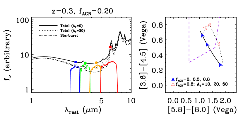
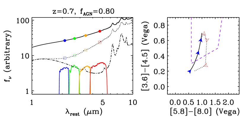
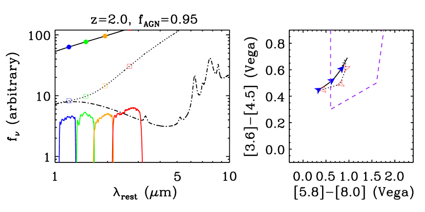
Figure 1.— Illustration of mid-IR AGN color selection. On the left, the solid lines show the rest-frame spectrum consisting of the sum of a starburst (Siebenmorgen & Krügel, 2007, dot-dashed lines) plus AGN power-law ($\alpha_{\nu}=-1$) templates. The three panels are for objects at $z=0.3$, 0.7, and 2, and AGN contribution to the rest-frame mid-IR (3–8 µm) emission $f_{\rm AGN}=0.2$, 0.8, and 0.95, respectively. Fluxes (shown by the filled circles) are determined by convolving the spectra with the responses of the four IRAC bands (shown). The dotted spectra and open squares in the left panels show the same model with the AGN power law extincted for $A_{V}=20$, with a Galactic extinction curve. The panels at right show corresponding locations on the color-color diagram for these models along with the S05 AGN color selection region. The solid lines in the color-color diagrams represent the colors as a function of increasing $f_{\rm AGN}$ from 0 to 0.95 for each redshift (the blue arrows show $f_{\rm AGN}=0$, 0.5 and 0.8). Note how increasing the contribution of the red AGN power law brings the objects into the S05 color selection region for all three redshifts, with the objects entering the selection region at $f_{\rm AGN}=0.3-0.5$. The dotted line in the right panel shows the effects of obscuration of the nuclear component (for $A_{V}=0-100$), for the spectrum with $f_{\rm AGN}=0.8$, with the open arrows representing $A_{V}=10$, 20, and 50. Very high dust extinction $A_{V}\sim 30$–50 will move the object out of the S05 selection region.

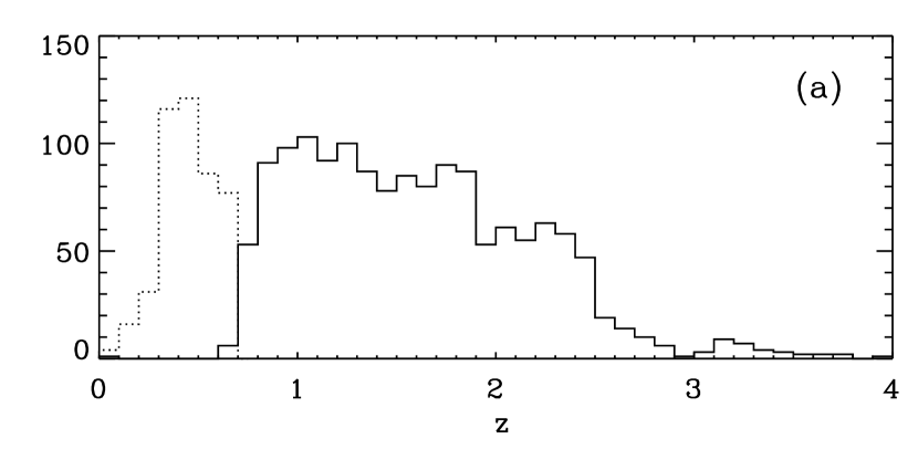
Figure 2.— Distributions of (a) redshift, (b) $L_{\rm 4.5\mu m}$, and (c) $L_{R}$ for the 1929 infrared-selected AGNs in the sample. $L_{\rm 4.5\mu m}$ and $L_{R}$ are $\nu L_{\nu}$ in the observed $R$ and IRAC 4.5 $\mu$m bands, respectively (see § 4.1). Many of the objects at $z<0.7$ (dotted line) are not AGNs but “normal” galaxies; above this redshift these objects are typically too faint to be detected in all four bands of the IRAC Shallow Survey. We restrict our analysis to the 1479 objects with $z>0.7$, shown by the solid line.

3. Infrared-selected AGN sample

The AGN sample used in this paper is selected in the mid-IR, which is less affected by obscuration than optical or soft X-ray emission. In the (rest-frame) near- to mid-IR from 1 to 10 $\mu$m, AGNs have markedly different SEDs from normal or starburst galaxies. AGNs typically have a roughly power law continuum in the near- to mid-IR, $S_{\nu}\propto\nu^{\alpha_{\nu}}$, where $\alpha_{\nu}\simeq-1$ (e.g., S05; Glikman et al., 2006). In contrast, normal and starburst galaxies have bluer continua in the rest-frame mid-IR, due to the fact that the spectrum from the stellar population of the galaxy peaks at $\simeq$1.6 $\mu$m, and falls at longer wavelengths. In addition, star-forming galaxies have prominent emission features at 3–10 $\mu$m due mainly to lines from polycyclic aromatic hydrocarbons (PAHs) in dust (Puget & Leger, 1989). This difference in SEDs allows us to effectively distinguish AGN-dominated objects from normal and starburst galaxies using observed colors in the mid-IR.

S05 developed a set of IRAC color-color selection criteria based on the IRAC Shallow Survey photometry and AGES spectra, described in § 2. In this paper we use those criteria to select AGNs. To illustrate the S05 color-color selection, we show in Fig. 1 the IRAC $[3.6]-[4.5]$ and $[5.8]-[8.0]$ colors for a two-component template spectrum consisting of a starburst galaxy (Siebenmorgen & Krügel, 2007) plus AGN power law with $\alpha_{\nu}=-1$. We show these colors for three redshifts and for various values of the fraction $f_{\rm AGN}$ of the rest-frame 3-10 $\mu$m luminosity that is emitted by the AGN. Because the colors of the power law AGN spectrum are constant with redshift, increasing $f_{\rm AGN}$ moves the colors into the S05 AGN selection region, regardless of the redshift of the source. Fig. 1 also shows the effect of dust extinction of the nuclear component, for a Galactic extinction curve (Pei, 1992). For $A_{V}\gtrsim 30$–50 (depending on redshift), extinction can cause the IRAC colors to move out of the S05 selection region, even for $f_{\rm AGN}$ as high as 0.8.

Table 1Matches of IRAC sources to AGES spectra and X-ray sources

	All IRAC		IRAGN ($z>0.7$)
AGES spectral type	All sources	X-ray	All sources	X-ray
Total	15492	1298	1479	654
BLAGN	941	592	697	457
NLAGN	108	43	4	2
Galaxies	5401	244	27	13
No spectrum	9042	419	751	182

We stress that this color-color technique does not select all AGNs. In the Boötes data (Gorjian et al., 2007), as well as the extended Groth strip (EGS; Barmby et al., 2006), only half of X-ray detected AGNs were identified using the S05 IRAC color-color criteria. This is likely due to the fact that some X-ray sources are too faint to be detected in all four IRAC bands, while others might not have red power-law mid-IR spectra. Recent mid-IR spectroscopy of type 2 quasars with the Infrared Spectrograph on Spitzer has shown that most luminous ($L_{\rm X}>10^{44}$ ergs s^-1) X-ray selected type 2 quasars have relatively featureless mid-IR spectra (Sturm et al., 2006; Weedman et al., 2006). Still, many AGNs in ultraluminous infrared galaxies (ULIRGs) show a variety of spectral shapes including PAH emission and deep silicate absorption features (Spoon et al., 2005; Buchanan et al., 2006; Brand et al., 2007), which may indicate deep obscuration of the nuclear IR emission. Therefore, the completeness of AGN color-color selection is still unclear. The key point for this study is that while color-color selection may miss many AGNs, there should be little contamination in the AGN color-color region from starburst-powered objects, particularly for objects with $z>0.7$ (see § 4.1). Sample completeness and contamination are discussed in more detail in § 7.

Our sample of IR-selected AGNs contains objects that have: (1) $5\sigma$ detections in all four IRAC bands as well as the $R$ band of the NOAO DWFS catalog, which we use to calculate optical luminosities; (2) IRAC colors that fall in the S05 AGN selection region; and (3) spectroscopic redshifts from AGES or photometric redshifts from the Brodwin et al. (2006) catalog, with $z_{\rm phot}>0$. These criteria select 1929 objects. Only 13 additional objects are not detected in the $R$ band but meet all the other criteria, so this requirement has little effect on our results. Excluding all objects with $z<0.7$ to minimize contamination by normal galaxies (see § 4.1) leaves a sample of 1479 IR-selected AGNs, of which 1469 have detections in all three NDWFS optical bands. Details of AGES spectra and X-ray matches to the objects are shown in Table 1.

4. Optical/IR SEDs and obscured AGN selection

In this section we calculate optical and IR luminosities for the IR-selected AGNs, and perform template fits to the optical and IR SEDs that provide evidence that roughly half of the sample has significant nuclear extinction. We then develop a simple optical-IR color criterion for selecting obscured AGNs. We show that the obscured AGN candidates display absorption in their average X-ray spectra and have the optical characteristics of normal galaxies, while the unobscured candidates are on average X-ray unabsorbed and have optical colors and morphologies typical of unobscured AGNs.

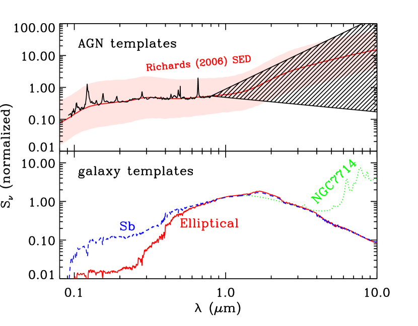
Figure 3.— Template spectra used for SED fits, normalized at 0.8 µm. The top panel shows the unabsorbed AGN template, with the mean SED and dispersion from Richards et al. (2006) for comparison. The hatched region at right shows the allowed values of $\alpha_{\nu}$. The bottom panel shows elliptical (red solid line), Sb (blue dashed line) and starburst (green dotted line) galaxy templates. See § 4.1 for details of the models.

4.1. Luminosities and model fits

For each of the 1479 AGNs in our sample, we calculate the observed mid-IR and optical luminosity densities using

$$L_{\nu}(\nu_{\rm rest})=\frac{4\pi d_{\rm L}^{2}}{1+z}S_{\nu}(\nu_{\rm obs}),$$ (1)

where $d_{\rm L}$ is the luminosity distance for a given redshift in our adopted cosmology (Hogg, 1999), $S_{\nu}$ is the flux density in ergs cm^-2 s^-1 Hz^-1, and $\nu_{\rm obs}$ and $\nu_{\rm rest}$ are the observed and rest-frame frequencies, respectively, where $\nu_{\rm rest}=(1+z)\nu_{\rm obs}$. Throughout the paper we present optical and IR luminosities in terms of the bolometric luminosity of the Sun, $L_{\sun}=3.83\times 10^{33}$ ergs s^-1.

We generally define luminosities and colors in terms of the observed (rather than rest-frame) photometric bands; the relationship between rest-frame luminosity density $L_{\nu}(\nu_{\rm rest})$ and the observed-frame luminosity density $L_{\nu}(\nu_{\rm obs})$ is

$$L_{\nu}(\nu_{\rm obs})=\frac{L_{\nu}(\nu_{\rm rest})}{(1+z)^{\alpha_{\nu}}},$$ (2)

where $\alpha_{\nu}$ is the power-law index ($S_{\nu}\propto\nu^{\alpha_{\nu}}$) for the spectrum between $\nu_{\rm obs}$ and $\nu_{\rm rest}$. Redshift estimates and detailed spectral shapes are uncertain for many of the AGNs in our sample, so framing the selection in terms of observed luminosities and colors makes our results less subject to the details of $K$-corrections.

We define luminosities in each photometric band in terms of $\nu L_{\nu}$, which unlike the luminosity density $L_{\nu}$, is not strongly affected by corrections for redshift, at least for unobscured quasars. Eqn. 2 shows that for a typical broadband quasar SED with IR power law with $\alpha_{\nu}=-1$, $\nu L_{\nu}$ remains constant with redshift. For a typical optical continuum (which is not exactly a power law, as described below), in the redshift range we consider ($0.7<z<3$), the observed $\nu L_{\nu}$ varies by at most 0.25 dex. In § 4.3, we estimate $K$-corrections and show that they have no significant effect on our selection criteria.

For the mid-IR luminosity we use $L_{\rm 4.5\mu m}$, defined to be $\nu L_{\nu}$ in the observed 4.5 $\mu$m IRAC band. Because the color-selected AGNs in our sample have similar IRAC SEDs, the $L_{\rm 4.5\mu m}$ is a simple and sufficiently accurate proxy for the total luminosity in the IRAC bands. In the optical, we use $L_{R}$, defined as $\nu L_{\nu}$ observed in the $R$ band centered on 6514 Å. The distributions of the 1929 IR-selected AGNs in redshift, $L_{\rm 4.5\mu m}$, and $L_{R}$ are shown in Fig. 2.

We restrict our sample to AGNs at $z>0.7$. At lower redshifts the IRAC source counts are dominated by normal or star-forming galaxies with relatively low luminosities ($L_{\rm 4.5\mu m}<10^{11}$ $L_{\sun}$). Some of these objects may have red IRAC SEDs, for example, due to heavy dust obscuration. The model SED from Siebenmorgen & Krügel (2007) for the heavily extincted starburst Arp 220 has IRAC colors that lie within the S05 AGN region, and less obscured sources can lie close to this region. Combined with photometric errors, this results in a significant number of $z<0.7$ objects selected with the S05 criterion being either normal or starforming galaxies. By cutting our sample at $z>0.7$, however, we exclude most of these “normal” galaxies as they are generally fainter than the flux density limits in the 5.8 µm, 8.0 $\mu$m, or $R$ bands (heavily extincted starbursts, for example, are very faint in the optical). In addition, limiting the sample to $z>0.7$ allows for more straightforward color selection of obscured AGNs, as shown in § 4.2. Our final IR-selected AGN sample includes only the 1479 IR-selected AGNs with $z>0.7$.

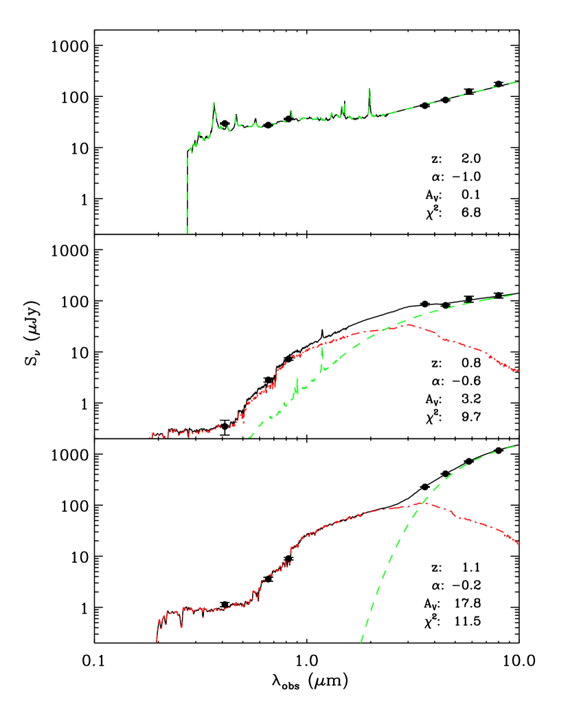
Figure 4.— Examples of fits to optical and IRAC photometry, for galaxy (red dot-dashed lines) and AGN (green dashed lines) spectral templates (see § 4.1 for a description of the models). These three example objects show a range of best-fit values to the AGN power-law slope $\alpha_{\nu}$ (where $S_{\nu}\propto\nu^{\alpha_{\nu}}$) and AGN template extinction $A_{V}$.

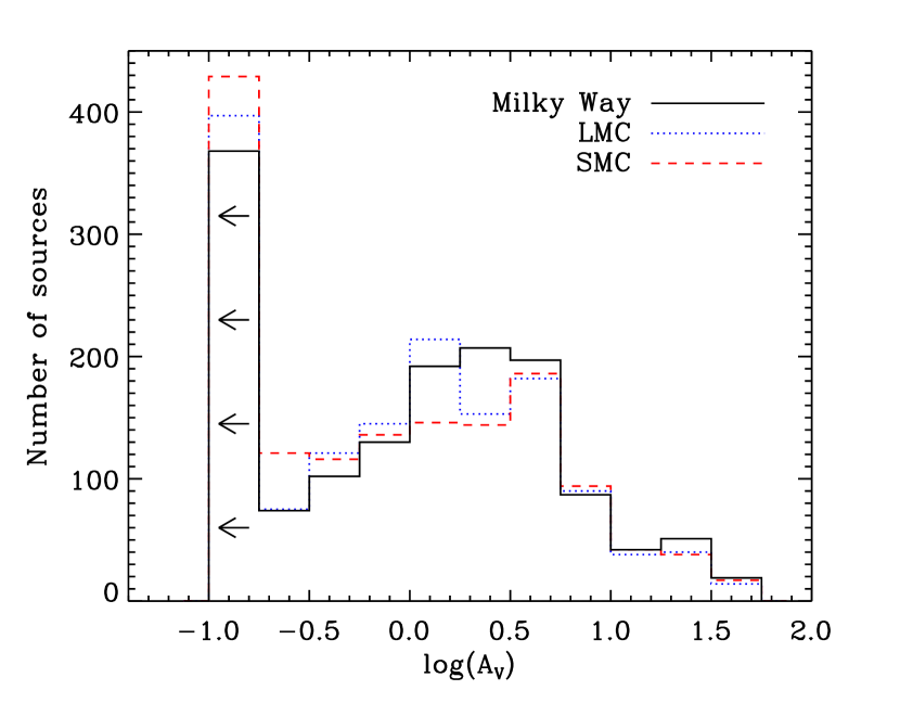
Figure 5.— Distribution of best-fit $A_{V}$ for the IR-selected AGNs. The far left bin corresponds to objects with $A_{V}\leq 0.2$. The three lines are for Galactic, LMC, and SMC extinction curves.

To model the SEDs of the IR-selected AGNs, we fit the optical and IRAC photometry of each source with spectral templates including AGN and host galaxy components. For the nuclear emission in the rest-frame optical/UV, we use the AGN template of Hopkins et al. (2007), which consists of the composite SED of Richards et al. (2006), with optical lines taken from the SDSS composite quasar template (Vanden Berk et al., 2001). For $\lambda>0.8$ $\mu$m, we use a power law component. Our grid of models includes 14 values of the slope from $-2.2\leq\alpha_{\nu}\leq 0.4$. We also include extinction of the nuclear component, with a Galactic extinction curve (Pei, 1992), and $E_{B-V}/A_{V}=3.1$ for 12 logarithmically spaced values of $0<A_{V}<32$. This corresponds to a total of 168 separate AGN models.

For the host galaxy emission, we use two model galaxy templates calculated using the PEGASE population synthesis code (Fioc & Rocca-Volmerange, 1997). The models are chosen so that at age 13 Gyr, they correspond to observed low-redshift ellipticals and spirals. The models differ in their initial specific star formation rates ($5\times 10^{-3}$ vs. $3.5\times 10^{-4}$ $M_{\sun}$ Myr^-1 per unit gas mass in $M_{\sun}$, for elliptical and Sb, respectively), the fraction of stellar ejecta available for new star formation (0.5 vs. 1), and extinction (none for the elliptical galaxy, disk extinction for the Sb). For simplicity, we use non-evolving spectra corresponding to an age of 3 Gyr after formation. Assuming that massive galaxies form at $z>6$, this age roughly corresponds to the age of such a galaxy at $z\sim 1$–2 for our adopted cosmology. At $\lambda>0.8$ $\mu$m, the models include either the quiescent galaxy spectrum, or the spectrum of the starburst galaxy NGC 7714 (Siebenmorgen & Krügel, 2007). This gives a total of four separate host galaxy models (E, Sb, E plus starburst, and Sb plus starburst). The quasar and galaxy template spectra are shown in Fig. 3.

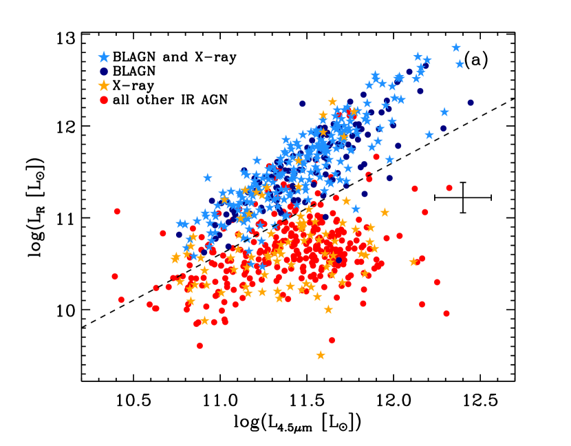
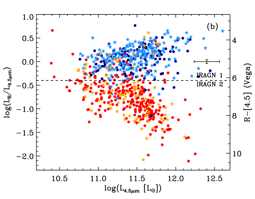
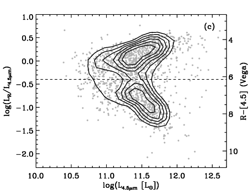
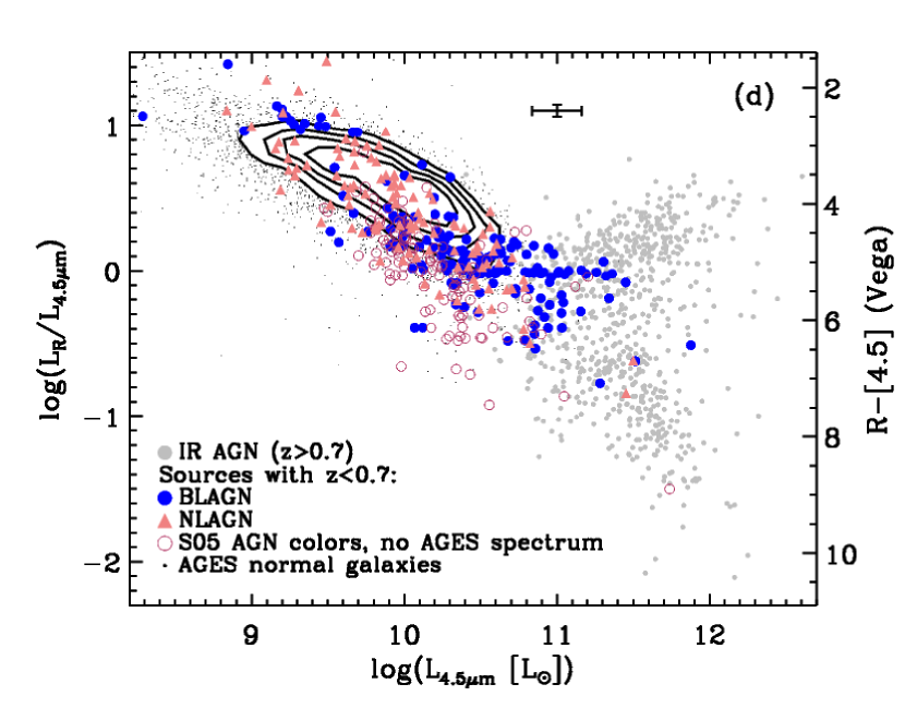
Figure 6.— (a) $L_{R}$ vs. $L_{\rm 4.5\mu m}$ and (b) $L_{R}/L_{\rm 4.5\mu m}$ vs. $L_{\rm 4.5\mu m}$ for IR-selected AGNs. Objects with optical spectroscopic classifications as BLAGNs are shown in blue, and X-ray sources are shown as stars. For clarity, only one out of every two objects is shown. Empirical selection criteria to separate IRAGN 1s and IRAGN 2s are shown by the dashed line. Error bars show the median uncertainties for objects lacking spectroscopic redshifts (objects with spectroscopic redshifts have much smaller uncertainties in luminosity). Luminosity uncertainties include both redshift and flux uncertainties; note that the error bars in (a) are not independent as the luminosity errors are dominated by uncertainty in $z$. (c) shows the same points as (b), but includes contours of source density that clearly show the bimodal distribution in $L_{R}/L_{\rm 4.5\mu m}$. (d) show the same distribution as (b), but includes sources at $z<0.7$ with various optical spectroscopic classifications.

For all AGN and galaxy models, we account for neutral hydrogen absorption in the intergalactic medium by setting the templates equal to zero blueward of the Lyman limit (912 Å), which is probed by the shortest-wavelength ($B_{W}$) band only for redshifts $z>2.7$. Additional absorption by Ly$\alpha$ becomes significant at $z\gtrsim 3$ and depends strongly on redshift; this absorption can be as strong as 50% at $\lesssim 4$. (e.g., Becker et al., 2007). However, only 42 (3%) of the objects in our sample lie at $z>3$, so for simplicity we ignore redshift-dependent Ly$\alpha$ absorption in our templates.

For each IR-selected AGN in our sample, we perform $\chi^{2}$ fits to the optical and IRAC photometry with the redshifted sum for each combination of starburst template and AGN power law (for this analysis we omit the 10 sources that do not have detections in all three NDWFS bands). We leave the normalizations of the AGN and galaxy components as free parameters, and we convolve the template spectra with the appropriate Mosaic-1 and IRAC response functions. From the template with the lowest $\chi^{2}$, we derive the best fit $\alpha_{\nu}$ and $A_{V}$ for the AGN. Example fits are shown in Fig. 4. From the best-fit template, we also calculate $K$-corrected luminosities $L_{2500\;\AA}$ and $L_{2\mu m}$, corresponding to the rest-frame $\nu L_{\nu}$ at 2500 Å, and 2 $\mu$m, respectively. These wavelengths are probed by the optical and IRAC photometry for all sources with $0.7<z<2.7$. The effects of $K$-corrections are discussed in § 4.3.

There is some evidence that the extinction in AGNs is best described by curves observed for the LMC and SMC, which have greater extinction in the UV than is observed in the Galaxy. To check the dependence of the fit parameters on the choice of extinction curve, we re-perform the SED fits using LMC and SMC curves (Pei, 1992). These do not significantly alter the quality of the fits, although the SMC curve gives somewhat lower $A_{V}$ estimates for some objects with $A_{V}\sim 1$.

4.2. Color selection of obscured AGNs

The distribution in the best-fit $A_{V}$ from the optical/IR SED fits is shown in Fig. 5. The AGN extinctions are bimodal, with a large fraction of sources having $A_{V}\gtrsim 1$, suggesting that the IRAC selection includes many obscured AGNs. We do not expect moderate extinction to strongly affect the IRAC color-color selection because the (rest-frame) near- and mid-IR emission that is probed with IRAC suffers relatively little obscuration by gas or dust compared to the optical, UV, or soft X-ray bands (although the near-IR can be extincted for sufficiently large $A_{V}$). As shown by the models in the lower two panels of Fig. 4, nuclear emission with significant extinction in the optical can still dominate over emission from the host galaxy in the IRAC bands. Because the extinction curve for the mid-IR is relatively flat (e.g., Pei, 1992; Indebetouw et al., 2005), extinction does not significantly affect the shape of the observed IRAC spectrum. Therefore, IRAC color-color selection can identify AGNs even for $A_{V}\sim 30$, as shown in Fig. 1.

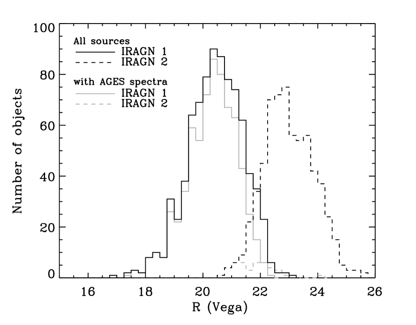
Figure 7.— Distribution in $R$ for the IRAGN 1 and IRAGN 2 subsets. Gray lines show the distribution for sources with AGES spectroscopy.

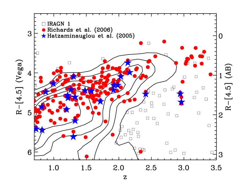
Figure 8.— Optical/mid-IR color ($R-[4.5]$) vs. redshift of IRAGN 1s, compared to type 1 AGN selected from other works. Note that blue colors are the top and red at the bottom, to correspond to the plots in Fig. 6. Squares and density contours are for IRAGN 1s. Red circles and blue stars show type 1 AGN from Richards et al. (2006) and Hatziminaoglou et al. (2005), respectively. The figure shows that most the color-selected IRAGN 1s show a similar distribution in color versus redshift as other samples, although our sample includes more moderately reddened AGNs (with $R-[4.5]>5.5$).

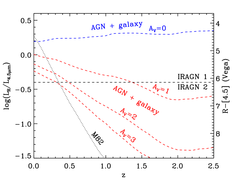
Figure 9.— $L_{R}/L_{\rm 4.5\mu m}$ vs. redshift for a template of AGN plus host galaxy (as described in § 4.1), with different values of the extinction on the AGN template. Because at higher $z$ the optical observations probe shorter wavelengths, where the extinction curve is steeper, $L_{R}/L_{\rm 4.5\mu m}$ varies more strongly with $A_{V}$. Therefore candidate obscured AGN can be more easily selected on the basis of optical-IR color at $z>0.7$, to which we restrict our sample. We also show, for comparison, the colors of a template for the starburst M82 (Siebenmorgen & Krügel, 2007), and the obscured AGN selection cut shown in Fig. 6.

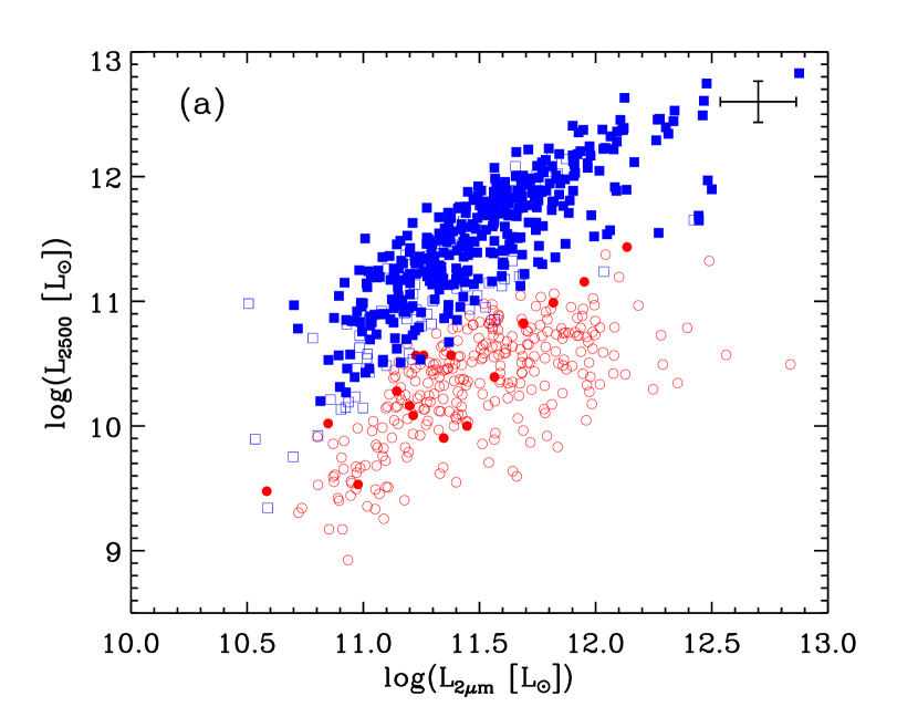
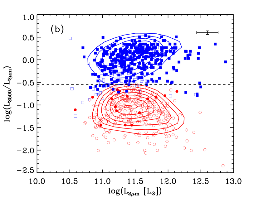
Figure 10.— Similar to Fig. 6, with $K$-corrected luminosities $L_{\rm 2500\;\rm\AA}$ and $L_{\rm 2\mu m}$ calculated from template fits (§ 4.1). IRAGN 1s (blue squares) and IRAGN 2s (red circles) are classified as defined in § 4.2 and shown in Fig. 6. For clarity, only one out of every two objects is shown. Filled symbols show objects with optical spectroscopic redshifts, while empty symbols have only photo-$z$’s. Errors are as in Fig. 6.

Since extinction by dust is much stronger in the optical than the IR, simple optical and IR color criteria (rather than detailed SED fits) can be used to select obscured objects. In Fig. 6 (a) we plot $L_{R}$ versus $L_{\rm 4.5\mu m}$ for the IR-selected AGNs. This plot shows two separate distributions of sources. The first has $L_{R}$ values that rise along with the $L_{\rm 4.5\mu m}$ and contains nearly all (96%) of the IR-selected AGNs that have optical spectra of BLAGNs. A total of 79% of these objects have relatively low extinction $(A_{V}<1)$ from the SED fits, so we associate them with candidate unobscured AGNs and classify them as type 1 IR-selected AGNs (IRAGN 1s). The second population has lower values of $L_{R}/L_{\rm 4.5\mu m}$, and 98% with $A_{V}\geq 1$, so we associate these with candidate obscured AGNs (IRAGN 2s). Unfortunately, spectroscopic classification is of little help with the IRAGN 2s, since most of them are fainter than the spectroscopic limits of AGES (Fig. 7). The 4% of the BLAGNs that lie in this “obscured” region have red colors in the optical, with $R-I\sim 0.7$–1.2, compared to $R-I\sim 0.3$ for a typical unreddened BLAGN.

We elucidate the distinction between the subsets by plotting the quantity $L_{R}/L_{\rm 4.5\mu m}$ (or equivalently in magnitudes, $R-[4.5]$) versus $L_{\rm 4.5\mu m}$ in Fig. 6 (b) and (c). The contours in Fig. 6(c) show that the distribution in $L_{R}/L_{\rm 4.5\mu m}$ is bimodal, so that there are two distinct populations. We empirically define the boundary between these two populations to be $\log{(L_{R}/L_{\rm 4.5\mu m})}=-0.4$, corresponding to $R-[4.5]=6.1$ (Vega) or $R-[4.5]=3.1$ (AB), as shown in all four plots in Fig. 6. We select this boundary (1) to divide the region populated by AGES BLAGNs from the region with few BLAGNs, and (2) to bisect the bimodal distribution in $L_{R}/L_{\rm 4.5\mu m}$ shown in Fig. 6(c). Because this boundary is based in part on the AGES spectral classifications, it is possible that our selection may be biased by the fact that AGES did not target optically fainter sources. However, as we show in § 5.1.3, X-ray analysis independently confirms the division at $\log{(L_{R}/L_{\rm 4.5\mu m})}=-0.4$. This criterion selects 839 IRAGN 1s and 640 IRAGN 2s.

The IRAGN 1s have mid-IR/optical colors similar to those found for other samples of type 1 AGNs. Fig. 8 shows the distribution in $R-[4.5]$ for the IRAGN 1s, with comparisons to samples from Richards et al. (2006) and Hatziminaoglou et al. (2005). Most of the IRAGN 1s show the same trend in redshift and color as these previous samples, although the IRAGN 1s include more moderately reddened AGNs (with $R-[4.5]>5.5$), which make up 24% of the total number of IRAGN 1s.

The color distribution in Fig. 6 can be interpreted in terms of how the observed $R$ and IRAC fluxes for AGNs change with extinction and redshift. In Fig. 9 we show $L_{R}/L_{\rm 4.5\mu m}$ versus $z$ for a template including an elliptical host galaxy plus AGN (with $\alpha_{\nu}=-1$ and various $A_{V}$) as described in § 4.1. The model AGN has an unabsorbed, rest-frame $R$-band luminosity 5 times that of the host galaxy. Fig. 9 shows that extinction of the AGN component decreases the observed $L_{R}/L_{\rm 4.5\mu m}$. This decrease becomes larger at higher $z$ because the $R$ band probes shorter wavelengths in the rest-frame UV, where dust extinction is greater. Because obscured AGNs at higher redshift tend to have higher $L_{\rm 4.5\mu m}$ (owing to the flux limits of the survey), more luminous objects appear redder in the observed $L_{R}/L_{\rm 4.5\mu m}$ for the same $A_{V}$. This explains the decrease in $L_{R}/L_{\rm 4.5\mu m}$ with $L_{\rm 4.5\mu m}$ observed in Figs. 6(b) and (c).

For starburst galaxies (shown by the M82 template), $L_{R}/L_{\rm 4.5\mu m}$ changes even more strongly with redshift; at low $z$, starbursts, obscured AGNs, and unobscured AGNs can have similar values of $L_{R}/L_{\rm 4.5\mu m}$. However, for most redshifts, all but the most extincted starbursts are not selected by the S05 IRAC color-color criteria; the colors for M82 and NGC 7714 fall in the S05 region only at $z\gtrsim 3$. We discuss possible contamination from these objects in § 7.3.

4.3. $K$-corrected colors

In Fig. 10 we include the $K$-corrections to the IR-selected AGN luminosities and plot $L_{2500\;\rm\AA}$ versus $L_{\rm 2\mu m}$. The $K$-corrections have negligible effect on the color classification; if we apply an equivalent empirical boundary to separate IRAGN 1s and 2s using the $K$-corrected luminosities [$\log{(L_{\rm 2500\;\AA}/L_{\rm 2\mu m})}=-0.55$, shown by the dashed line in Fig. 10], only 90 of the 1479 objects (6%) change their classification. Therefore, almost all the IRAGNs can be empirically classified by their observed colors, independent of $K$-corrections, which allows this criterion to be used for samples that do not include accurate redshifts.

4.4. Dependence of color selection on luminosity and redshift

The template used in Fig. 9 represents a luminous AGN that dominates the optical emission from the host galaxy. For lower-luminosity AGNs, whose unobscured optical flux is smaller than that of their hosts, extinction of the nucleus will have a relatively small effect on $L_{R}/L_{\rm 4.5\mu m}$. Therefore, our selection criterion is not applicable for samples of sources at lower luminosities and redshifts. In Fig. 6(d), we show $L_{R}/L_{\rm 4.5\mu m}$ versus $L_{\rm 4.5\mu m}$ for subsets of objects at $z<0.7$, for comparison to the $z\geq 0.7$ IRAGN sample. At low $L_{\rm 4.5\mu m}$, optical BLAGNs and NLAGNs have $L_{R}/L_{\rm 4.5\mu m}$ typical of normal galaxies, indicating that their total emission is dominated by the hosts, and this simple color criterion cannot distinguish obscured sources.

By cutting our IRAGN sample at $z=0.7$, we include only sources with $L_{\rm 4.5\mu m}\gtrsim 10^{11}$ $L_{\sun}$ (owing to the flux limits of the IRAC Shallow Survey). These AGNs are luminous enough that if unobscured, their nuclear optical luminosity is comparable to all but the most luminous host galaxies. Therefore, our redshift cut at $z\geq 0.7$ enables obscured AGN color selection, (1) by probing shorter rest-frame wavelengths in the optical and (2) by selecting luminous AGNs for which the intrinsic optical luminosity is larger than the host.

4.5. Are the IRAGN 2s intrinsically optically faint?

We consider the possibility that the IRAGN 2s are not obscured, but intrinsically faint in the observed optical band. For example, there exist modes of accretion that lack a luminous accretion disk and therefore do not radiate strongly in the optical and UV; these are known as radiatively inefficient accretion flows (e.g., Narayan & Yi, 1995). However, in such a scenario it is difficult to explain the observed properties of IRAGN 2s in the mid-IR. The red IRAC colors and high mid-IR luminosities of these objects are characteristic of dust that has been heated to high temperatures by high UV fluxes, and so imply some luminous UV emission from the nucleus. Such emission would not be present in radiatively inefficient flows. Therefore, we hypothesize that all the IRAGN 2s are intrinsically luminous enough in the UV to power the observed mid-IR emission, but they are optically faint because the nuclear emission is obscured.

4.6. Bolometric luminosities

A fundamental property of AGNs is the bolometric accretion luminosity $L_{\rm bol}$. For the IRAGN 2s, the nuclear optical light is extincted, and most objects are not individually detected in X-rays, so we cannot use optical or X-ray luminosities to estimate $L_{\rm bol}$. Instead, we derive $L_{\rm bol}$ by scaling from the $K$-corrected luminosity of the AGN at 2 µm, $L_{\rm 2\mu m}^{\rm AGN}$, taken from the SED fits (§ 4.1). $L_{\rm bol}$ is given by $L_{\rm bol}=BC_{2\rm\mu m}L_{\rm 2\mu m}^{\rm AGN}$, where $BC_{2\rm\mu m}$ is the bolometric correction. We derive $BC_{2\rm\mu m}$ from the luminosity-dependent quasar SED model of Hopkins et al. (2007), for which the correction is in the range $BC_{2\rm\mu m}=10$–15 for the luminosities of the sample (we note that the luminosity-independent model of Richards et al. (2006) gives a similar $BC_{2\rm\mu m}=12$).

The distributions in $L_{\rm bol}$ are shown in Fig. 11. The $L_{\rm bol}$ values of (0.1–10)$\times 10^{46}$ ergs s^-1 are similar for IRAGN 1s and 2s and are typical of the accretion luminosities of bright Seyferts and quasars. We see no systematic difference between the distributions for the two types of IRAGNs, indicating that at these high luminosities, the fraction of obscured to unobscured sources is relatively constant with luminosity. However, these results give only approximate distributions in $L_{\rm bol}$ because of uncertainties in the photo-$z$’s for individual objects, particularly IRAGN 2s (see § 6). While it would be very interesting to use this sample to study quantities such as the evolution of the obscured AGN fraction with $z$ or $L_{\rm bol}$, to confidently perform such measurements requires better calibration of the IRAGN 2 redshifts.

Figure 11.— Distribution in bolometric luminosity $L_{\rm bol}$ estimated as described in § 4.6, for the two types of IR-selected AGN.

5. Multiwavelength tests of obscured AGN selection

Our classification of candidate AGNs as unobscured (IRAGN 1) or obscured (IRAGN 2) is based solely on the ratio of their observed optical to IR color. This classification makes several predictions for the observed emission from these sources at X-ray, optical, and infrared wavelengths:

1. The average X-ray properties of the two populations should be consistent with unabsorbed and absorbed AGNs, respectively. Both types should have high X-ray luminosities typical of Seyferts and quasars. The IRAGN 1s should have X-ray spectral shapes consistent with unabsorbed AGNs, while $>$70%–80% of the IRAGN 2s should have harder X-ray spectra due to absorption by neutral gas (e.g., Tozzi et al., 2006).

2. For IRAGN 2s, the observed X-ray absorption should be consistent with the extinction derived from the optical/UV colors, for a reasonable gas-to-dust ratio.

3. The IRAGN 1s and 2s should have optical morphologies and optical colors characteristic of BLAGNs and galaxies, respectively.

In §§ 5.1–5.3 we test each of these predictions using the available data from Chandra, Spitzer, and optical photometry and spectroscopy. In each case we show that the data are consistent with the above classification of IR-selected AGNs as unobscured (IRAGN 1) and obscured (IRAGN 2).

5.1. X-ray properties

Table 2Average X-ray fluxes from stacking

	Number	0.5–2 keV		2–7 keV
Subset	of sources	Counts source-1	Flux source-1	Counts source-1	Flux source-1	$HR$
All sources
IRAGN 1s	346	$7.64\pm 0.15$	$9.90\pm 0.19$	$2.76\pm 0.09$	$10.9\pm 0.4$0	$-0.47\pm 0.02$
IRAGN 2s	267	$2.48\pm 0.10$	$3.21\pm 0.12$	$1.65\pm 0.08$	$6.50\pm 0.31$	$-0.20\pm 0.03$
Normal galaxies	2107	$0.49\pm 0.02$	$0.63\pm 0.02$	$0.33\pm 0.01$	$1.30\pm 0.05$	$-0.19\pm 0.03$
Non X-ray detected sources
IRAGN 1s	122	$0.92\pm 0.09$	$1.20\pm 0.11$	$0.47\pm 0.06$	$1.86\pm 0.25$	$-0.32\pm 0.08$
IRAGN 2s	179	$0.41\pm 0.05$	$0.53\pm 0.06$	$0.46\pm 0.05$	$1.83\pm 0.20$	0$0.06\pm 0.09$
Normal galaxies	2011	$0.12\pm 0.01$	$0.15\pm 0.01$	$0.08\pm 0.01$	$0.33\pm 0.03$	$-0.17\pm 0.05$

X-ray emission is an efficient and largely unbiased way of detecting AGN activity for objects with $N_{\rm H}\lesssim 10^{24}$ cm^-2 (for reviews see Mushotzky, 2004; Brandt & Hasinger, 2005). Thus, the contiguous Chandra coverage of the Boötes field provides a useful diagnostic for confirming our classifications of IR-selected AGNs (S05; Gorjian et al., 2007), allowing us to estimate both the X-ray luminosity $L_{\rm X}$ and the absorbing neutral hydrogen column density $N_{\rm H}$.

The main limitation of the wide-field XBoötes observations is that they are shallow, with exposures of only 5 ks yielding a 0.5–7 keV source flux limit of $(4-8)\times 10^{-15}$ ergs cm^-2 s^-1. Most IR-selected AGNs do not have firm X-ray detections, and most detected sources have fewer than 10 counts, so we do not have X-ray spectral information for most individual sources. We therefore perform a stacking analysis, which compensates for the shallowness of the X-ray observations by averaging over the large number of IR-selected AGNs in the field. By summing X-ray images around the known IR positions, we determine the average X-ray fluxes, luminosities and spectral shapes of various subsets of these sources.

5.1.1 X-ray stacking

Around the position of each object in a given sample, we extract $40\times 40$-pixel (19.7″) X-ray images in the soft band (0.5–2 keV) and hard band (2–7 keV). Because the Chandra telescope PSF varies with angle $\theta$ from the optical axis, the aperture from which we extract source photons varies from source to source. We take this aperture to be the 90% energy encircled radius at 1.5 keV:

$$r_{90}\simeq 1\arcsec+10\arcsec(\theta/10\arcmin)^{2}.$$ (3)

We include in the stacking analysis only objects that lie within 6′ of the optical axis of a Chandra pointing, for which $r_{90}<4\farcs 6$. This excludes over half the available sources but minimizes source confusion and maximizes signal-to-noise ratio. Using a model of the Chandra PSF (from the Chandra CALDB) and sources with random positions inside the 6′ radius, an aperture of $r_{90}$ includes 90%–92% of the source counts in both the 0.5–2 keV and 2–7 keV bands. Accordingly, in our stacking analysis, we multiply the observed source counts by 1.1 to obtain the total counts from the source.

Of the 126 pointings in the XBoötes data set, there are eleven that have significantly higher background intensities, due to background flares (for a detailed discussion of ACIS backgrounds see Hickox & Markevitch, 2006). In our stacking analysis, we do not include any source positions that lie within these eleven “bad” exposures. The total area over which we perform the stacking, which consists of the region covered by IRAC that lies within the central 6′ radii of these 115 pointings, is 2.9 deg².

An accurate measure of the stacked source flux requires subtraction of the background, which we estimate by stacking X-ray images on random positions around the Boötes field, at least 20″ away from any X-ray sources included in the XBoötes catalog (Kenter et al., 2005). We performed 20 trials, stacking $\sim$30,000 positions in each trial. As a check, we also calculate the surface brightness using the ACIS blank-sky data sets, which are obtained using deep exposures at high Galactic latitude and removing all detected sources.

Both estimates of the diffuse background give identical surface brightnesses of 3.0 counts s^-1 deg^-2 in the 0.5–2 keV band and 5.0 counts s^-1 deg^-2 in the 2–7 keV band. We use these values to calculate the expected background counts within a circle of radius $r_{90}$ for each source position. For a typical $r_{90}=3$″ and an exposure time of 4686 s (see below), this corresponds to 0.03 and 0.05 background counts for each IRAC source in the 0.5–2 keV (soft) and 2–7 keV (hard) bands, respectively.

Subtracting this background, we obtain the average X-ray flux in counts source^-1. We assume that all source positions have an X-ray exposure time of 4686 s, which is the mean for all the XBoötes observations excluding the “bad” exposures. For simplicity we ignore variations in exposure time between pointings, as well as variations in effective exposure time within each single ACIS-I field of view due to mirror vignetting. These variations are at most $\sim$10% and do not significantly affect our results. We convert count rates (in counts s^-1) to flux (in ergs cm^-2 s^-1) using the conversion factors $6.0\times 10^{-12}$ ergs cm^-2 count^-1 in the 0.5–2 keV band and $1.9\times 10^{-11}$ ergs cm^-2 count^-1 in the 2–7 keV band. In addition to fluxes, we obtain rough X-ray spectral information by calculating the hardness ratio, defined as

$${\rm HR}=\frac{H-S}{H+S},$$ (4)

where $H$ and $S$ are the count rates in the hard and soft bands, respectively. Errors in count rates are calculated using the approximation $\sigma_{X}=\sqrt{X+0.75}+1$, where $X$ is the number of counts in a given band (Gehrels, 1986). Uncertainties in HR are derived by propagating these count rate errors. In the following analysis, we use these hardness ratios and fluxes to determine the typical absorption and X-ray luminosities from the stacking analysis.

Figure 12.— Verification of IRAGN 2 selection using X-ray data. Shown is the average hardness ratio from X-ray stacking analysis, for objects with $L_{\rm 4.5\mu m}<3\times 10^{11}$ $L_{\sun}$, in bins of $\log{(L_{R}/L_{\rm 4.5\mu m})}$. The dashed line shows the boundary between IRAGN 1 and 2 as defined in Fig. 6.

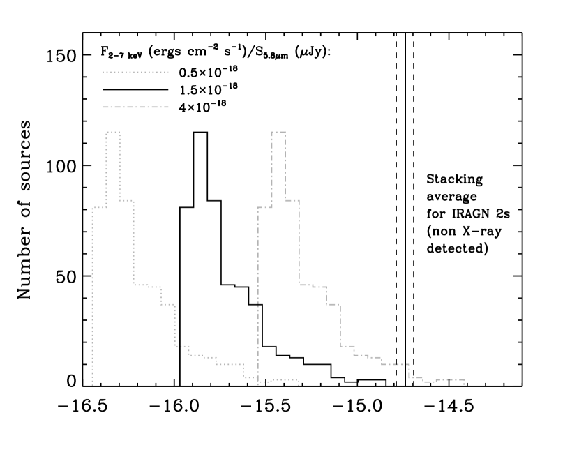
Figure 13.— Comparison of average 2–7 keV flux for X-ray undetected IRAGN 2s, versus X-ray fluxes expected for star formation. Vertical lines show observed average 2–7 keV X-ray flux from stacking analysis of $\langle F_{\rm 2-7\;keV}\rangle=(1.83\pm 0.20)\times 10^{-15}$ ergs cm^-2 s^-1 (Table 2). Histograms show the distribution of predicted X-ray fluxes for star formation, given the measured $S_{\rm 5.8\mu m}$ for each object and the ratio $F_{\rm 2-7\;keV}/S_{\rm 5.8\mu m}$ for star formation (see Eqn. 6), derived from the $F_{\rm 2-10\;keV}/F_{\rm FIR}$ relation of Ranalli et al. (2003), and typical starburst SEDs. The three histograms represent $F_{\rm 2-7\;keV}/S_{\rm 5.8\mu m}=(0.5-4)\times 10^{18}$ ergs cm^-2 s^-1 $\mu$Jy^-1, for which the average values of $F_{\rm 2-7\;keV}$ are $(0.8-6)\times 10^{-16}$ ergs cm^-2 s^-1. Even for the largest typical ratio of X-ray to 5.8 $\mu$m flux, the observed average flux is $>3$ times larger than that expected for star formation. This indicates that the X-ray emission from these objects is dominated by nuclear accretion.

Table 3X-ray properties of IR-selected AGNs versus redshift

	Number	${\rm rms}(d_{\rm L})$	0.5–2 keV	$\langle L_{\rm 0.5-2\;keV}\rangle$	2–7 keV	$\langle L_{\rm 2-7\;keV}\rangle$
$z$	of sources	(Gpc)	(counts src-1)	($10^{43}$ ergs s-1)	(counts src-1)	($10^{43}$ ergs s-1)	$HR$
IRAGN 1 (all sources)
0.7–1.0	65	0$5.52\pm 0.03$	$11.9\pm 0.4$0	$5.3\pm 0.2$	$4.4\pm 0.3$	$6.5\pm 0.4$	$-0.46\pm 0.03$
1.0–1.5	125	0$8.76\pm 0.03$	$7.6\pm 0.3$	$8.2\pm 0.3$	$2.5\pm 0.2$	$9.1\pm 0.5$	$-0.50\pm 0.03$
1.5–2.0	86	$13.1\pm 0.1$	$4.4\pm 0.2$	$10.3\pm 0.6$0	$1.7\pm 0.2$	$13.2\pm 1.2$0	$-0.44\pm 0.04$
2.0–2.5	45	$17.5\pm 0.1$	$4.3\pm 0.3$	$17.1\pm 1.3$0	$1.9\pm 0.2$	$25.0\pm 3.0$0	$-0.39\pm 0.06$
IRAGN 2 (all sources)
0.7–1.0	31	$5.6\pm 0.2$	$1.7\pm 0.3$	$0.8\pm 0.1$	$1.9\pm 0.3$	$2.8\pm 0.5$	0$0.04\pm 0.11$
1.0–1.5	69	$8.6\pm 0.2$	$2.3\pm 0.2$	$2.5\pm 0.2$	$1.8\pm 0.2$	$6.3\pm 0.7$	$-0.13\pm 0.06$
1.5–2.0	72	$13.2\pm 0.3$0	$3.1\pm 0.2$	$7.2\pm 0.6$	$1.7\pm 0.2$	$13.6\pm 1.5$0	$-0.28\pm 0.06$
2.0–2.5	76	$18.2\pm 0.5$0	$1.9\pm 0.2$	$8.0\pm 0.8$	$1.0\pm 0.1$	$14.7\pm 2.0$0	$-0.28\pm 0.07$
IRAGN 1 (non X-ray detected sources)
0.7–1.0	15	$5.5\pm 0.1$	$0.63\pm 0.28$	$0.28\pm 0.12$	$0.67\pm 0.29$	$0.97\pm 0.41$	0$0.03\pm 0.31$
1.0–1.5	39	$8.9\pm 0.1$	$0.94\pm 0.18$	$1.05\pm 0.20$	$0.49\pm 0.14$	$1.79\pm 0.51$	$-0.32\pm 0.16$
1.5–2.0	36	$13.0\pm 0.1$0	$0.86\pm 0.18$	$1.99\pm 0.43$	$0.40\pm 0.14$	$3.06\pm 1.04$	$-0.37\pm 0.17$
2.0–2.5	21	$17.4\pm 0.2$0	$0.87\pm 0.26$	$3.47\pm 1.02$	$0.37\pm 0.19$	$4.92\pm 2.47$	$-0.40\pm 0.24$
IRAGN 2 (non X-ray detected sources)
0.7–1.0	19	$5.6\pm 0.2$	$0.18\pm 0.16$	$0.08\pm 0.07$	$0.32\pm 0.19$	$0.49\pm 0.29$	0$0.28\pm 0.49$
1.0–1.5	49	$8.7\pm 0.2$	$0.36\pm 0.11$	$0.38\pm 0.12$	$0.52\pm 0.12$	$1.82\pm 0.45$	0$0.19\pm 0.19$
1.5–2.0	41	$13.2\pm 0.4$0	$0.34\pm 0.12$	$0.80\pm 0.28$	$0.30\pm 0.11$	$2.32\pm 0.89$	$-0.07\pm 0.26$
2.0–2.5	53	$18.2\pm 0.5$0	$0.42\pm 0.11$	$1.82\pm 0.48$	$0.50\pm 0.12$	$7.09\pm 1.72$	0$0.08\pm 0.17$

Figure 14.— Results from X-ray stacking analysis, in bins of redshift, for IRAGN 1s and 2s. Here all sources are included, including those with X-ray detections. Shown are the average $L_{\rm X}$ in the (a) 2–7 keV, and (b) 0.5–2 keV bands, and (c) average hardness ratio. Note that the IRAGN 2s are consistently harder (larger HR) than the IRAGN 1s.

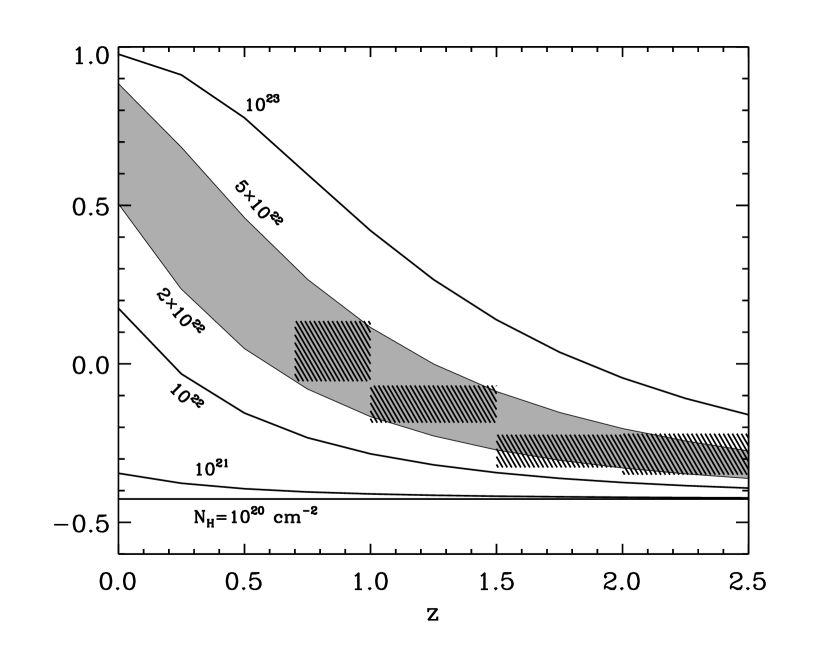
Figure 15.— X-ray hardness ratio HR vs. redshift for various $N_{\rm H}$ (given in cm^-2), given an intrinsic power-law photon index $\Gamma=1.8$ and the on-axis ACIS response function. Hatched regions show the observed $1\sigma$ limits in HR for the IRAGN 2s in bins of redshift, as shown in Fig. 14. Assuming the intrinsic $\Gamma=1.8$, these HR values for IRAGN 2s are consistent with a constant $N_{\rm H}=$(2–5)$\times 10^{22}$ cm^-2, shown by the shaded region.

Figure 16.— Same as Fig. 14, only including sources with no detections in the XBoötes catalog (Kenter et al., 2005). X-ray undetected IRAGNs have average $L_{\rm 0.5-7\;keV}\sim 10^{43}$ ergs s^-1 characteristic of luminous Seyfert galaxies. The X-ray undetected IRAGN 2s have systematically larger average hardness ratios than the X-ray undetected IRAGN 1s.

5.1.2 Calculation of $N_{\rm H}$ and $L_{\rm X}$

Measuring $N_{\rm H}$ and $L_{\rm X}$ from X-ray fluxes requires an assumption for the X-ray spectrum of the source, which for most AGNs can be modeled by a simple power law with photon index $\Gamma$, such that the photon flux density (in photons cm^-2 s^-1 keV^-1) $F\propto E^{-{\Gamma}}$. For all the AGNs in our sample, we assume an intrinsic X-ray spectrum with $\Gamma=1.8$, typical for unabsorbed AGNs (Tozzi et al., 2006); as we show in § 5.1.3, this $\Gamma$ corresponds to the average spectral shape of the IRAGN 1s. Although X-ray AGNs do not all have the same intrinsic $\Gamma$, the typical intrinsic spectrum does not vary significantly with luminosity or $N_{\rm H}$ (Tozzi et al., 2006). Therefore, it is reasonable to assume a constant $\Gamma$ when estimating $N_{\rm H}$ and $L_{\rm X}$ for an ensemble of sources.

Given a constant intrinsic X-ray spectrum, $N_{\rm H}$ is directly related to the observed hardness ratio. Absorption by neutral gas preferentially obscures lower energy X-rays, and so a larger $N_{\rm H}$ corresponds to a larger (in this case, less negative) HR. The conversion between HR and $N_{\rm H}$ depends on the response function of the X-ray detector and the redshift of the source. With increasing $z$, the low-energy turnover due to absorption by neutral hydrogen is increasingly redshifted out of the 0.5–2 keV bandpass. Therefore, for a power-law spectrum attenuated by a fixed column density of gas, the observed spectrum will become softer with increasing redshift, so that objects with higher $z$, but equal HR, correspond to greater absorption. Assuming $\Gamma=1.8$, we have calculated HR for a grid of absorptions ($10^{20}\leq N_{\rm H}\leq 10^{23}$ cm^-2) and redshifts ($0\leq z\leq 4$), and will use these to convert observed hardness ratios to column densities. Note that the Galactic $N_{\rm H}$ toward this field is very small ($\sim$$10^{20}$ cm^-2), so we neglect it in our estimates of column density.

To derive the average $L_{\rm X}$ and $N_{\rm H}$ from stacking requires an estimate of redshift, so we perform the stacking in bins of $z$. For each bin we calculate the rms value of $d_{\rm L}$ for the objects in the bin. Using this distance, along with the average fluxes from stacking, we calculate $\langle L_{\rm X}\rangle$ in each bin. We also include a $K$-correction to $\langle L_{\rm X}\rangle$, assuming $\Gamma=1.8$, to account for the fact that the X-ray bands we observe probe higher energies in the rest-frame spectrum. This $K$-correction varies from 0.9 at $z=0.7$ to 0.8 at $z=2$, so it has a relatively small effect on $\langle L_{\rm X}\rangle$.

5.1.3 Average X-ray fluxes

As a first step in the stacking analysis, we compare the average X-ray fluxes of different subsets of sources in the Boötes catalog. We divide the sources into (1) IRAGN 1s and (2) IRAGN 2s, defined by $L_{R}/L_{\rm 4.5\mu m}$ as shown in Fig. 6, and for comparison (3) objects with detections in all four IRAC bands that are identified as optically normal galaxies in the optical from their AGES spectra. The IRAGNs are all selected to have $z>0.7$, while the optically normal galaxies mainly lie at $z<0.7$. In interpreting X-ray stacking results, it is a concern that the X-ray brightest objects may dominate the average flux. Therefore, we perform the stacking analysis twice, first using all objects in each subsample and then using only those objects that are not detected with 4 or more counts in the XBoötes source catalog (Kenter et al., 2005).

Average fluxes in the soft and hard bands are given in Table 2. Including all sources, the IRAGN 1s have a larger average 2–7 keV flux than the IRAGN 2s, with $\langle F_{\rm 2-7\;keV}\rangle=10.9\times 10^{-15}$ and $6.5\times 10^{-15}$ ergs cm^-2 s^-1 source^-1, respectively. However, when we exclude those objects that are detected in the XBoötes catalog, the hard X-ray fluxes of the two subsets closely agree. This suggests that the IRAGN 1 sample contains more bright X-ray sources than the IRAGN 2 sample, but for faint sources ($<$4 counts), the two IRAGN types have similar average fluxes.

While the hard X-ray fluxes are comparable between the IRAGN 1s and 2s, the soft X-ray fluxes are significantly smaller for the IRAGN 2s, indicating that they are more absorbed. The IRAGN 1s have an average $HR=-0.47$, which is close to that expected for an unabsorbed AGN with $\Gamma=1.8$. In contrast, the IRAGN 2s have $HR=-0.20$. The optically normal galaxies have $HR=-0.19$, similar to the IRAGN 2s, but with $\sim$5 times smaller average flux.

As mentioned in § 4.2, the X-ray data can be used to verify our selection criterion for IRAGN 1s and 2s, by looking for systematic differences in HR (and thus absorption) on either side of our selection boundary. We can therefore address concerns that the selection may be biased by the AGES spectroscopic flux limits, especially for $L_{\rm 4.5\mu m}<3\times 10^{11}$ $L_{\sun}$, where the distribution in $L_{R}/L_{\rm 4.5\mu m}$ is not as clearly bimodal (Fig. 6). We perform the stacking analysis in bins of $L_{R}/L_{\rm 4.5\mu m}$ for the IRAGNs with $L_{\rm 4.5\mu m}<3\times 10^{11}$ $L_{\sun}$ and plot HR versus $L_{R}/L_{\rm 4.5\mu m}$ in Fig. 12. There is a significant increase in HR across our IRAGN 1/IRAGN 2 boundary of $\log{L_{R}/L_{\rm 4.5\mu m}}=-0.4$, verifying that this criterion effectively separates objects with unabsorbed (IRAGN 1) and absorbed (IRAGN 2) X-ray emission and is not significantly affected by the AGES flux limits.

Next, to confirm that the X-ray flux for these objects comes from nuclear emission, we show that the average X-ray flux is significantly larger than that expected for star formation. The X-ray flux $F_{X}$ from star formation is related to the far-IR flux $F_{\rm FIR}$ (see Eqn. 12 of Ranalli et al., 2003). $F_{\rm FIR}$ is defined as (Helou et al., 1985)

$$F_{\rm FIR}=1.26\times 10^{-11}(2.58S_{60\mu{\rm m}}+S_{100\mu{\rm m}}){\rm\>ergs\>cm^{-2}\>s^{-1}},$$ (5)

where $S_{60\mu{\rm m}}$ and $S_{100\mu{\rm m}}$ are in Jy. For the suite of starburst model SEDs given in Siebenmorgen & Krügel (2007), we calculate the ratio of rest-frame $F_{\rm FIR}$ (in ergs cm^-2 s^-1) to the observed flux at 5.8 $\mu$m, $S_{\rm 5.8\mu m}$ (in $\mu$Jy). Excluding Arp 220 (which has an extreme star formation rate and is highly extincted in the optical, so it would not be detected in our survey), we find that $F_{\rm FIR}/S_{\rm 5.8\mu m}\sim(0.3-2)\times 10^{-14}$ ergs cm^-2 s^-1 $\mu{\rm Jy}^{-1}$ for the redshift range $0.7<z<3$. Combining with the Ranalli et al. (2003) relation and converting from the rest-frame 2–10 keV band luminosity to our observed 2–7 keV band flux using a $\Gamma=1.8$ power law spectrum (with the appropriate small $K$-correction), we have

$$F_{\rm 2-7\;keV}=S_{\rm 5.8\mu m}\times(0.5-4)\times 10^{-18}{\rm\;ergs\;cm^{-2}\>s^{-1}\>\mu Jy^{-1}}$$ (6)

Making the conservative assumption that the observed 5.8 µm flux for every IRAGN 2 is due entirely to stars and star formation, we can put an upper limit on the $F_{\rm 2-7\;keV}$ we expect from star formation for each object. The distribution in these $F_{\rm 2-7\;keV}$ values, for every IRAGN 2 that is not detected in X-rays, is shown in Fig. 13. By comparison, the average $F_{\rm 2-7\;keV}$ observed for these objects is $>3$ times larger than that typically expected for star formation, even for the largest typical ratio of X-ray to 5.8 $\mu$m flux. This confirms that for most of the IRAGN 2s, the X-ray emission is not powered by star formation, but nuclear accretion.

5.1.4 Average $L_{\rm X}$ and $N_{\rm H}$

In order to use the X-ray stacking analysis to measure physical parameters such as the accretion luminosity ($L_{\rm X}$) or the gas attenuation ($N_{\rm H}$), we must include redshift information. Therefore, we have repeated the stacking for both types of IRAGN in bins of redshift from $z=0.7$–2.5. We do not include sources at $z>2.5$ because we do not have enough objects with best-fit $z>2.5$ to obtain well-constrained fluxes. We stress here that although there may be significant uncertainties in photometric redshift estimates, particularly for IRAGN 2s, there is no large bias in the photo-$z$’s, as we show in § 6. Therefore, our stacking analysis using large bins in redshift should not be strongly affected by photo-$z$ uncertainties.

The stacking results as a function of $z$ are listed in Table 3, and we plot $\langle L_{\rm X}\rangle$ versus $z$ in Fig. 14. For both IRAGN types, $\langle L_{\rm X}\rangle$ increases by a factor of $\sim$2 between $z=0.5$ and $z=2.5$, due to the evolution in the quasar luminosity function with redshift (e.g., Ueda et al., 2003; Barger et al., 2005; Hasinger et al., 2005) and the IR and optical flux limits that restrict us to selecting only the most luminous objects at high $z$. The $\langle L_{\rm 2-7\;keV}\rangle$ range (0.3–3)$\times 10^{44}$ ergs s^-1 is typical for Seyfert galaxies and quasars and much larger than the typical $L_{\rm X}$ of starburst or normal galaxies. Although the IRAGN 2s have $\langle L_{\rm 0.5-2\;keV}\rangle$ and $\langle L_{\rm 2-7\;keV}\rangle$ that are 3–5 and 2–3 times lower than the IRAGN 1s, respectively, these $L_{\rm X}$ values are still typical of AGNs and not starburst galaxies.

Plotting HR in redshift bins (Fig. 14), the IRAGN 2s are significantly harder at all $z$. The IRAGN 1s have $HR\simeq-0.45$ for all $z$, which corresponds to an intrinsic $\Gamma=1.8$ with no absorption. The IRAGN 2s are significantly harder, with $HR\simeq-0.3$–0.1. Assuming that these have the same intrinsic $\Gamma$ as the IRAGN 1s, we estimate the corresponding $N_{\rm H}$. In Fig. 15 we plot HR versus $z$ for several values of $N_{\rm H}$ assuming $\Gamma=1.8$. The hatched regions correspond to the $1\sigma$ errors in HR for the IRAGN 2s in each of our redshift bins. For all redshifts, the IRAGN 2 HR values are consistent with a column density of $N_{\rm H}=$(2–5)$\times 10^{22}$ cm^-2, marked by the shaded region in Fig. 15.

As mentioned in the previous section, it is a concern that the average $L_{\rm X}$ and $N_{\rm H}$ we measure may be dominated by a few bright sources. To address this, we repeat the stacking as a function of $z$ but exclude those objects that are detected in the XBoötes catalog. The results are shown in Fig. 16 and indicate that even those objects that are not detected in X-rays have $\langle L_{\rm X}\rangle$ values consistent with AGNs. In addition, the IRAGN 2s have harder spectral shapes than the IRAGN 1s, even at these fainter fluxes.

To summarize the X-ray stacking results, both IRAGN types have average X-ray fluxes that are too large to be due to star formation and thus strongly indicate AGN activity. Performing the stacking as a function of redshift, we find that both IRAGN 1s and 2s have average $L_{\rm X}$ values consistent with Seyferts and quasars, and the IRAGN 1s have hardness ratios consistent with unabsorbed AGNs ($\Gamma=1.8$). The IRAGN 2s, assuming the same intrinsic spectrum, correspond to absorbed sources with $N_{\rm H}\sim 3\times 10^{22}$ cm^-2.

5.2. Gas absorption and dust extinction

In this section, we check that the dust extinction for the IRAGN 2s that we inferred from the optical/UV data is consistent with the $N_{\rm H}$ we measure in X-rays, assuming that, in general, the X-ray-absorbing gas is coincident with the extincting dust. Fig. 5 shows that the SEDs of most of the IRAGN 2s are best fitted by templates with $0.7<A_{V}<7$. The ratio of gas to dust in the Galaxy is such that $N_{\rm H}/A_{V}\simeq 2\times 10^{21}{\;\rm cm}^{-2}$, or $A_{V}\simeq 15$ for the observed average $N_{\rm H}=3\times 10^{22}$ cm^-2. This extinction is more than enough to obscure the optical light from the nucleus, although it is somewhat larger than the typical $A_{V}$ obtained from the SED fits.

However, there is evidence that AGNs have high gas-to-dust ratios, similar to or perhaps even greater than that of the SMC (see Fall & Pei, 1989; Martínez-Sansigre et al., 2006, and references therein). The SMC has $N_{\rm H}/A_{V}\simeq 2\times 10^{22}{\;\rm cm}^{-2}$, which corresponds to $A_{V}\simeq 1.5$ for the observed average $N_{\rm H}$ and is close to the typical $A_{V}$ obtained by the SED fits to the IRAGN 2s. Therefore, we conclude that the dust extinction implied by the optical and IR observations is generally consistent with the average $N_{\rm H}$ we derive from X-ray stacking.

The bimodality in the $A_{V}$ distribution from SED fits (Fig. 5), as well as the clear separation of the two IRAGN types in optical-IR color (Fig. 6), suggests that there is a bimodal distribution in the dust column density to the IR-selected AGNs. There is no obvious selection effect that could produce this bimodality, so we expect that it is real. This is broadly consistent with previous results on the distribution of $N_{\rm H}$ measured in X-rays. These studies find many objects with $N_{\rm H}<3\times 10^{20}$ cm^-2 or $N_{\rm H}>3\times 10^{21}$ cm^-2, with relatively few at intermediate column densities (e.g. Treister & Urry, 2005; Tozzi et al., 2006). However, such a bimodal distribution could simply be due to limitations of X-ray spectral fitting techniques, with which it is difficult to measure $N_{\rm H}$ as low as $\sim 10^{21}$ cm^-2, especially at high redshifts where X-ray telescopes probe energies higher than the photoelectric cutoff at $E\simeq 1$ keV (e.g., Akylas et al., 2006). The colors we observe in IR-selected AGNs suggests that such a bimodal obscuration distribution does indeed exist, which has implications for models of AGN obscuration, as we discuss in § 8.3.

Figure 17.— Optical morphologies for the two types of IR-selected AGNs. (a) Histograms of the $I$ band stellarity parameter ${\tt CLASS\_STAR}$ output by ${\tt SExtractor}$ (0 for extended sources, 1 for point sources). Note that the vast majority of IRAGN 1s are point-like, while the IRAGN 2s are extended, suggesting that their optical emission is dominated by the nucleus and by the host galaxy, respectively. (b) Variation of $I$ band ${\tt CLASS\_STAR}$ with $I$ magnitude, for the flux range in which the two IRAGN subsets overlap. The $y$ axis shows the fraction of sources that have $I>0.5$ in each magnitude bin. Errors shown are counting statistics, and only bins with $>$5 sources are shown. The point-like fraction does not vary with $I$ and is significantly different between the two subsets.

5.3. Optical morphologies and colors

Since we expect the nuclear optical emission from the IRAGN 2s to be extincted, their optical light should be dominated by their host galaxies. Normal galaxies differ from quasars in optical images in two principal ways: (1) galaxies have extended morphologies, while quasars are dominated by a small nucleus and so appear as point sources; and (2) normal galaxies have redder colors, characteristic of a composite stellar spectrum rather than a blue AGN continuum. By examining the optical morphologies and colors of our IRAGN sample, we can confirm that optical emission is dominated by an AGN in IRAGN 1s and by the host galaxy in IRAGN 2s.

To quantify morphologies, we use the ${\tt CLASS\_STAR}$ parameter output by the ${\tt SExtractor}$ photometry code (Bertin & Arnouts, 1996). ${\tt CLASS\_STAR}$ is a measure of how well an object can be approximated by a point source, with values ranging from 0 (extended) to 1 (point source). In Fig. 17 (a), we plot the distribution in ${\tt CLASS\_STAR}$ in the $I$ band (which best discriminates between the two IRAGN types) and find that 74% of the IRAGN 1s have ${\tt CLASS\_STAR}$ $>0.7$, indicating that the emission is point-like, while 85% of the IRAGN 2s have ${\tt CLASS\_STAR}$ $<0.5$, indicating mainly extended emission.

However, for very faint objects, it is possible to obtain low ${\tt CLASS\_STAR}$ values, even if the sources are point-like. Therefore, we must confirm that the lower ${\tt CLASS\_STAR}$ values for IRAGN 2s are not simply a result of their lower fluxes. Fig. 17 (b) shows the fraction of objects with ${\tt CLASS\_STAR}>0.5$ for each IRAGN subset as a function of $I$ magnitude. There is no clear trend in this fraction with $I$ for the IRAGN 2s, and for the magnitudes in which the subsets overlap, the IRAGN 2s have many fewer “point-like” morphologies than the IRAGN 1s. We conclude that the IRAGN 2s do have more extended morphologies than the IRAGN 1s, so that the color selection described in § 4.2 can effectively distinguish between objects dominated by a nucleus and those dominated by extended emission.

Table 4Best template fits to optical photometry

	Best-fit template
Subset	Elliptical	Sb	Quasar
optical BLAGN	170	362	402
optical NLAGN	71	35	0
optical galaxies	4103	1167	47
IRAGN 1	143	327	368
IRAGN 2	452	168	11

Note. — Includes sources with detections in all three optical bands ($B_{W}$, $R$, and $I$) and all four IRAC bands.

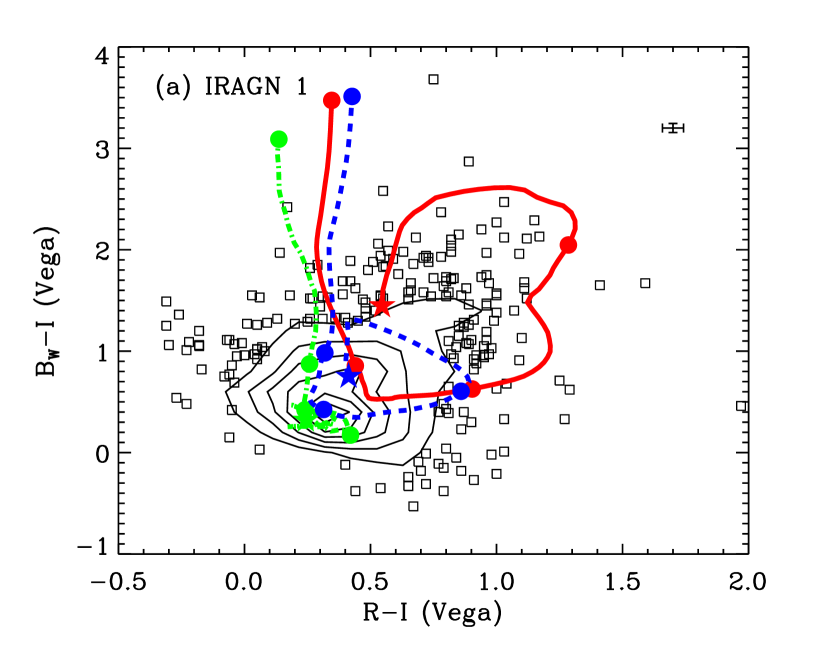
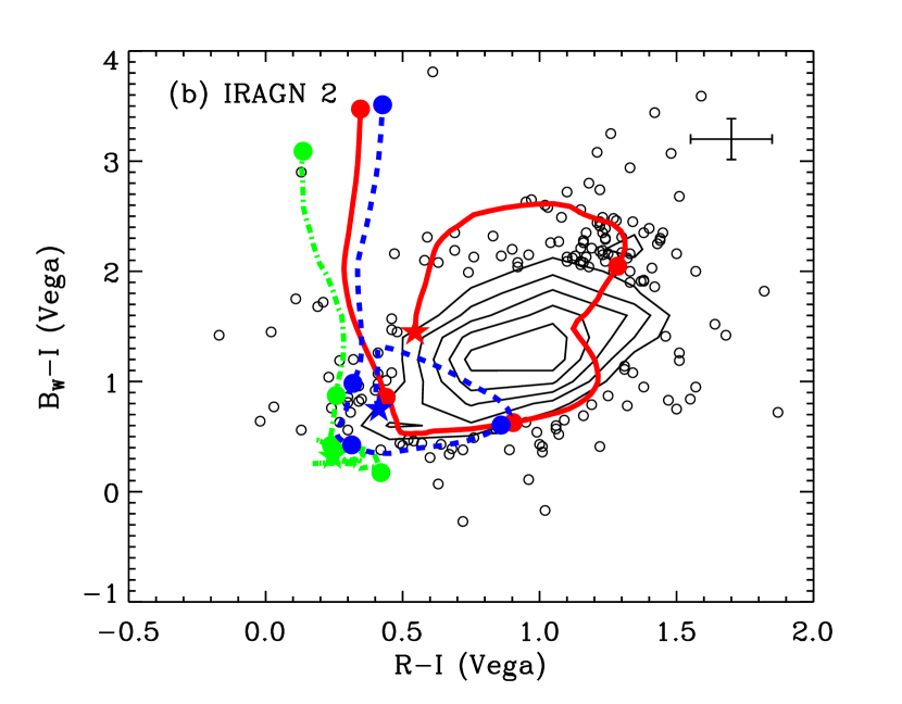
Figure 18.— Contours and points show observed $B_{W}-R$ and $R-I$ colors for (a) IRAGN 1s and (b) IRAGN 2s, compared to colors for elliptical galaxy (red solid line), Sb galaxy (blue dashed line), and quasar (green dot-dashed line) templates. The model tracks run from $z=0-4$. Stars show the color at $z=0$, and filled dots indicate $z=1$, 2, 3, and 4. Error bars show the median uncertainty in the colors for objects lacking spectroscopic redshifts.

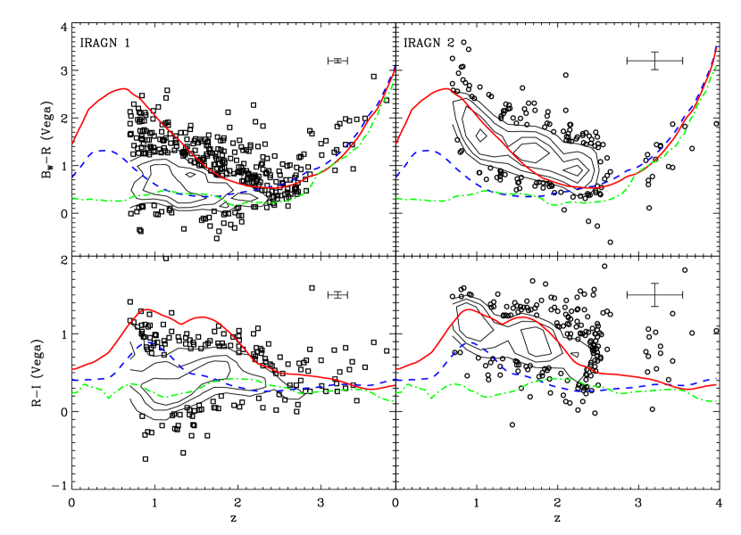
Figure 19.— Contours and points show observed $B_{W}-R$ and $R-I$ colors for IRAGN 1s (top) and IRAGN 2s (bottom) versus redshift, compared to model tracks as in Fig. 18. Error bars show the median uncertainty in the colors for objects lacking spectroscopic redshifts.

We also examine the observed $B_{W}-R$ and $R-I$ colors of the two IRAGN types and compare them to the colors of the galaxy and quasar templates described in § 4.1. In Fig. 18 we plot the $B_{W}-R$ versus $R-I$ color tracks for the templates as a function of redshift and overplot the observed colors for the two IRAGN types. As expected, most IRAGN 1s have colors resembling a quasar spectrum, although there are a few objects (even those with optical BLAGN spectra) that have redder colors, owing to some optical extinction. By comparison, the IRAGN 2s as a whole have colors that are redder than those of the IRAGN 1s and lie between the elliptical and spiral redshift tracks. Fig. 19 shows a similar plot, but as a function of redshift. Again we see that the IRAGN 2s have colors and trends with redshift that are closer to optically normal galaxies than to quasars.

To quantify this further, we fit the quasar, elliptical, and Sb templates (shown in Fig. 3) to the $B_{W}$, $R$, and $I$ photometry for the 1469 IR-selected AGNs with detections in all three optical bands. For comparison, we perform the same fits for objects at all redshifts that have four-band $5\sigma$ IRAC detections and AGES classifications as BLAGN, NLAGN, and galaxies (as listed in the first column of Table 1). We fix the redshift of the template spectrum and leave only the normalization as a free parameter. The distribution of templates that fit the photometry with the lowest $\chi^{2}$ is shown in Table 4. A total of 695 (83%) of the IRAGN 1s are best fitted by the quasar or Sb templates (which have similar colors for $z>1.5$), similar to the fits for optical BLAGNs. By contrast, 452 (71%) of the IRAGN 2s are best fitted by the elliptical template, with almost all the rest fit by the Sb template, similar to the fits for optical NLAGNs and optically normal galaxies. We conclude that the IRAGN 2s, as a population, do indeed have optical colors consistent with host galaxies and are markedly different from the IRAGN 1s.

6. Verification of photometric redshifts

The selection criteria developed here for IRAGN 2s depend only on observed color and so are independent of redshift. However, our SED fits and luminosity calculations depend on redshift, so it is important to verify our redshift estimates. Of the 1479 objects in our IR-selected AGN sample, 751 have no spectroscopic redshift, so for these we use photo-$z$’s calculated from IRAC and optical photometry. As described in Brodwin et al. (2006), photo-$z$’s using template-fitting techniques generally fail for objects such as the IR-selected AGNs that have featureless, power law SEDs. To overcome this difficulty, the technique of Brodwin et al. (2006) uses an artificial neural net to estimate the photo-$z$’s for such objects, using those objects that also have spectroscopic redshifts as a training set.

However, only 42 of the 640 IRAGN 2s have spectroscopic redshifts and thus are included in the training set. As shown in Fig. 7, most of the IRAGN 2s are too faint to be spectroscopically targeted in AGES. Therefore, it is not immediately clear that photo-$z$ estimates, which are calibrated against a training set of optically brighter objects (many of them optical BLAGNs), will also be valid for the IRAGN 2s that have significantly different mid-IR to optical SEDs. It is encouraging that the average X-ray hardness ratio for the IRAGN 2s decreases with redshift as expected for a small range in $N_{\rm H}$ (Fig. 15). However, the sharp cutoff at $z\simeq 2.5$ in the redshift distribution of the IRAGN 2s (visible in Fig. 19) suggests a possible systematic bias in the $z_{\rm phot}$. It is important to verify that such errors do not significantly affect our results.

6.1. Comparison of spectroscopic and photometric redshifts

As a first check, we compare the photometric versus spectroscopic redshifts for the IRAGNs, as shown in Fig. 20. For completeness, this figure includes all objects selected by the S05 IRAC criteria (including those with $z<0.7$), but it does not include 38 IRAGN 1s that have AGES spectroscopy but do not have well-constrained photo-$z$’s from the Brodwin et al. (2006) catalog. For the IRAGNs, the distribution in $\delta z=(z_{\rm phot}-z_{\rm spec})/(1+z_{\rm spec})$ is roughly Gaussian, with mean, dispersion, and fraction of outliers (objects outside $2\sigma$ in the distribution) of -0.03, 0.16, and 0.06, respectively. These values are (-0.03, 0.15, 0.05) for the 648 IRAGN 1s separately and (-0.06, 0.18, 0.10) for the 42 IRAGN 2s, indicating reasonably good agreement for both IRAGN types.

The distribution in $\delta z$ is skewed somewhat by $\sim 20$ quasars at $z_{\rm spec}>2$ and $z_{\rm phot}<1$. The presence of these sources suggests that for some high-$z$ IRAGN, our reliance on photo-$z$’s may give a large underestimate for the redshift (some such objects would be eliminated from the sample by our requirement that $z>0.7$). Fig. 20 also includes 73 sources with $z_{\rm phot}>0.7$ and $z_{\rm spec}<0.7$, indicating that there could be $\sim$10% contamination from low-$z$ sources in the IRAGN sample. Still, 54 of these 73 sources have $z_{\rm spec}>0.5$, so the contamination from very low redshifts ($z<0.5$) is expected to be $\lesssim 3$%. In addition, the sample includes 33 sources ($\sim$5%) with $z_{\rm phot}<0.7$ and $z_{\rm spec}>0.7$ that would not be included in the IRAGN sample.

Other redshift estimates in the Boötes field come from Houck et al. (2005), who obtained redshifts for 17 optically-faint sources using the Infrared Spectrograph on Spitzer. Of these, 5 have $5\sigma$ detections in the IRAC bands, and 4 have IRAC colors inside the S05 selection region. These four sources have photo-$z$ estimates from the Brodwin et al. (2006) catalog, although only two are in our IRAGN 2 sample (the other two have no detection in the $R$ band). Of the IRAGN 2s, one has $R=23.8$ and $(z_{\rm spec},z_{\rm phot})=(1.95,2.35)$ while the other has $R=24.7$ and $(2.59,3.96)$. The two sources with no $R$ counterpart have $(0.70,0.99)$ and $(1.75,1.01)$. Based on only these four objects it is difficult to make any conclusions about the whole sample, except that photo-$z$’s are more uncertain for fainter sources.

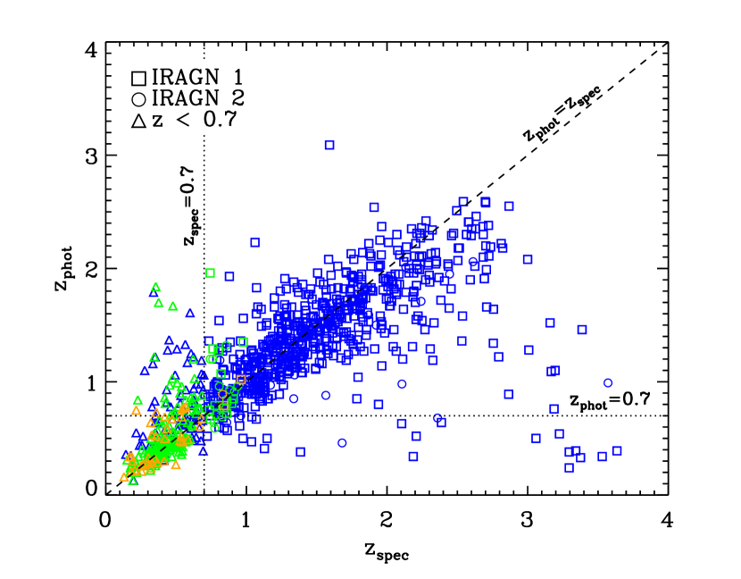
Figure 20.— Photometric redshifts ($z_{\rm phot}$) from the Brodwin et al. (2006) catalog versus spectroscopic redshifts ($z_{\rm spec}$), for those objects with AGES optical spectra. Squares show IRAGN 1s, circles show IRAGN 2s. BLAGNs are shown in blue, NLAGNs are shown in orange, and optically normal galaxies are shown in green. The dashed line corresponds to $z_{\rm phot}=z_{\rm spec}$, while the dotted lines show $z_{\rm spec}=0.7$ and $z_{\rm phot}=0.7$. Objects with no optical spectrum and with $z_{\rm phot}<0.7$ would not be included in the IRAGN sample.

Figure 21.— Verification of Brodwin et al. (2006) photo-$z$’s ($z_{\rm phot}$) for IRAGN 2s using three-band optical galaxy template redshifts ($z_{\rm temp}$). The dashed line corresponds to $z_{\rm temp}=z_{\rm phot}$. Filled points have spectroscopic redshifts, while open points have only photo-$z$’s; note that we plot $z_{\rm phot}$ here even for objects with spectroscopic redshifts.

6.2. Comparison to optical template redshifts

To test the photo-$z$’s for the entire IRAGN 2 sample, we note that most IRAGN 2s have galaxy-like optical colors (§ 5.3). Therefore, for these sources we can perform a rough template photo-$z$ estimate by using only the optical photometry, fitting the $B_{W}$, $R$, and $I$ SED as in § 5.3, but allowing the redshift to vary.

The accuracy of the template fits is limited by the fact that we have only three optical photometric data points, so that the fits are underdetermined if they include too many free parameters. We have tried fits using a wide range of galaxy and starburst templates with varying ages and extinctions, and consistently find that if we include two or more templates, the photo-$z$’s are poorly constrained. We therefore use a single, non-evolving template, of which the elliptical galaxy model described in § 4.1 provides the best constraints over the wide range in redshift ($0.7<z\lesssim 3$) covered by our sample.

The best-fit redshifts ($z_{\rm temp}$) from these template fits are shown in Fig. 21. The $z_{\rm temp}$ estimates follow the Brodwin et al. (2006) empirical photo-$z$’s reasonably well and cover the same range in redshift, except for a group of 80 objects that have very low $z_{\rm temp}<0.1$ (we note, however, that most of these sources have a second minimum in the $\chi^{2}$ function that lies within $\pm 0.5$ of the $z_{\rm phot}$). Excluding the sources with $z_{\rm temp}<0.1$, 79% of the IRAGN 2s have $\left|z_{\rm temp}-z_{\rm phot}\right|<0.25(1+z_{\rm phot})$, with a bias toward lower redshifts at $1.7<z<2.2$. Objects with $z_{\rm phot}\sim 2.5$ have a wide range in $z_{\rm temp}$, which may indicate that the real redshift distribution of the IRAGN 2s extends smoothly out to $z\gtrsim 3$, similar to the IRAGN 1 sample.

We also obtain similar results with the ${\tt HyperZ}$ photometric redshift package (Bolzonella et al., 2000), using the same fixed, non-evolving template spectrum. These results give us confidence that the IRAGN 2s lie at redshifts $0.7\lesssim z\lesssim 3$ and that the photo-$z$’s have no systematic bias large enough to significantly affect the physical interpretation of our results.

7. Sample contamination and completeness

In the previous section we showed that our mid-IR and optical color classification for obscured AGNs is verified by the typical X-ray, IR, and optical properties of these objects. Therefore, we are confident in the general technique of selecting obscured AGNs. However, to make estimates of how our IRAGN 2 sample relates to the total population of obscured AGNs, it is important to address issues of contamination and completeness.

7.1. Photometric uncertainties and color selection

We first address the photometric uncertainty in the IRAC colors that are used to select the IRAGN. Photometric error will lead some sources to move into or out of the S05 selection region, causing contamination or incompleteness, respectively. These will be dominated by the 5.8 and 8 µm IRAC bands, which are less sensitive than the shorter wavelength bands; the $1\sigma$ uncertainty in the $[5.8]-[8.0]$ color is typically in the range $0.1-0.4$, compared to $0.02-0.08$ for $[3.6]-[4.5]$.

The color-color distribution indicates that incompleteness is a greater problem than contamination. Fig. 22(a) shows the IRAC color-color distribution, highlighting those objects with $S_{5.8}/\sigma_{5.8}>15$, where $\sigma_{5.8}$ is the error in the 5.8 µm band flux. This shows that the bright sources in the S05 AGN region occupy a small locus in color-color space around a line defined by

$$[3.6]-[4.5]=0.2([5.8]-[8.0])+1.8.$$ (7)

The spread of points about this line is consistent with the photometric uncertainties. For all sources lying above the lower boundary in the S05 criteria (shown as black points in Fig. 22(a), we derive the difference $\Delta C$ between the observed $[5.8]-[8.0]$ and the line defined above. The distribution in $\Delta C/\sigma_{C}$, where $\sigma_{C}$ is the $1\sigma$ uncertainty in the color, is shown in Fig. 22(b), and is well fitted by a Gaussian with mean $-0.04$ and $\sigma=1.05$. This indicates that most of the objects with high $[3.6]-[4.5]$ can be associated with the S05 region and in fact may occupy a remarkably tight locus in color-color space. However, photometric errors cause $\sim$10% to be observed outside the AGN selection region. Conversely, we only expect $\sim$100 sources to be scattered into this region, indicating that contamination due to photometric errors is $\lesssim$5%.

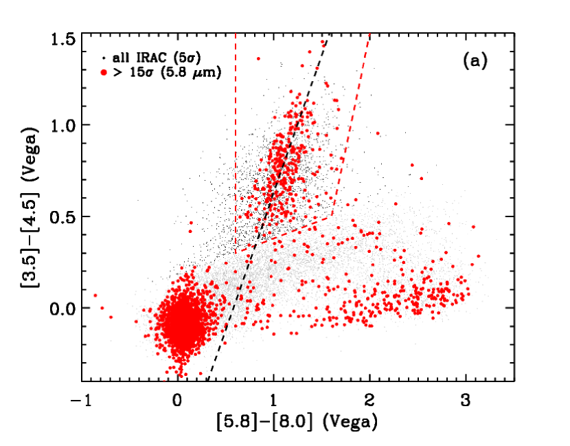
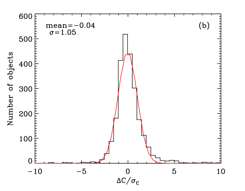
Figure 22.— (a) IRAC color-color distribution for the $\approx$15,500 IRAC sources with four-band $5\sigma$ detections. We have excluded from this figure 139 stars that are brighter than the saturation limits given in Eisenhardt et al. (2004); all have $[5.8]-[8.0]<0.4$ and so do not lie in the S05 AGN selection region (shown by the red dashed line). Sources with $[3.6]-[4.5]$ greater than the lower boundary of the S05 region are shown in black. Objects with $S_{5.8}/\sigma_{5.8}>15$ are shown in red, and the locus defined by these points (Eqn. 7) is shown by the diagonal line. (b) Distribution of the deviation ($\Delta C$) of $[5.8]-[8.0]$ colors from the diagonal line for the black points in (a), in units of the $1\sigma$ uncertainty in the $[5.8]-[8.0]$ color. A Gaussian fit to the distribution is shown in red, and is consistent with most points having intrinsic colors defined by the line shown in (a).

7.2. Reliability of obscured AGN selection

It is important to estimate the reliability of our classification of IRAGNs based on IR-optical colors; that is, how many IRAGN 1s are actually obscured, and how many IRAGN 2s are unobscured? In the sample of 839 IRAGN 1s, 719 have BLAGN spectra from the AGES data set, or have point-like optical morphologies (${\tt CLASS\_STAR}>0.7$) and are best fitted by blue (quasar or Sb) optical templates. These are strong indicators that a source is an unobscured, type 1 AGN, so the color selection is at least 85% reliable for IRAGN 1s. Of the 640 IRAGN 2s, 517 have galaxy-like optical colors and ${\tt CLASS\_STAR}\leq 0.5$, and do not have BLAGN optical spectra (only 29, or 3%, of the IRAGNs with BLAGN spectra are classified as IRAGN 2s). These criteria only indicate that an object is dominated by the host galaxy in the optical; however, as discussed in § 4.2, the high IRAC luminosities of these sources would suggest dominant nuclear emission in the optical, were they unobscured. We conclude that our selection of obscured AGNs based on optical-IR color is at least 80% reliable.

7.3. Contamination from starburst and normal galaxies

We expect almost all of the IRAGN 1s to be AGNs rather than starburst or normal galaxies. Most of these objects were targeted by AGES, so we can verify their classification with optical spectra. Of the 686 IRAGN 1s that have AGES spectroscopy (or 82% of the IRAGN 1 sample), 668 (97%) are BLAGNs, while 3 are NLAGNs and 15 are optically normal galaxies. Keeping in mind that many AGES targets were selected to be X-ray sources and thus are biased toward bright AGNs, we consider separately the 233 IRAGN 1s that have optical spectra but no X-ray counterpart. These should be a representative sample of the IRAGN 1s that are not detected in X-rays, and of these 226 (97%) are BLAGNs, one is a NLAGN, and five are optically normal galaxies. We conclude that there is little ($<$5%) contamination in the IRAGN 1 sample.

It is more difficult to estimate contamination in the IRAGN 2s. Only 42 IRAGN 2s have AGES spectra (29 BLAGNs, 1 NLAGN, 12 galaxies), because most IRAGN 2s are fainter than the AGES flux limits (Fig. 7). A total of 155 of the IRAGN 2s have X-ray detections and thus $L_{\rm X}$ values that imply that they must be powered by accretion. Of the remaining 485 objects, some at high redshifts might not be AGNs but instead luminous starburst galaxies with IRAC colors that lie inside the S05 AGN color-color selection region. As mentioned in § 4.1, heavily extincted starbursts (i.e., Arp 220) can have very red IRAC colors. However, the Siebenmorgen & Krügel (2007) Arp 220 template is also very red in the optical ($B_{W}-I>3$ at $z>0.7$), which is much redder than observed for the IRAGN 2s (Fig. 19). Still, it is possible that some high-$z$ starbursts have similar IRAC colors to Arp 220 but are bluer in the optical, and these could contaminate the IRAGN 2 sample. In addition, at $z\gtrsim 3$, the colors of less obscured starbursts (e.g., M82) would also lie in the S05 region (see Fig. 6 of Barmby et al., 2006). However, to be detected to our IRAC flux limits at $z>3$, a source must have a very high $L_{\rm 5.8\mu m}>10^{12}$ $L_{\sun}$ (where $L_{\rm 5.8\mu m}$ is the observed $\nu L_{\nu}$ in the 5.8 µm band). For a typical ratio of rest-frame far-infrared (FIR) to observed 5.8 µm fluxes for starburst galaxies (§ 5.1.3), this implies $L_{\rm FIR}\gtrsim 10^{13}$ $L_{\sun}$. In most such “hyperluminous infrared galaxies”, a significant (and often dominant) contribution to the IR emission comes from an AGN (e.g., Farrah et al., 2002). Also considering that our IRAGN sample contains only 27 objects at $z>3$ that do not have BLAGN optical classifications, contamination from such high-$z$ starbursts should be small.

One empirical constraint on contamination comes from the X-ray stacking results, due to the fact that starburst galaxies tend to be significantly fainter in the X-rays than AGNs. If we exclude sources that have X-ray counterparts, the IRAGN 1s and 2s have similar average X-ray fluxes in the 2–7 keV band of $0.47\pm 0.06$ and $0.46\pm 0.05$ counts source^-1, respectively (Table 2). Because there is little contamination in the IRAGN 1 sample, 0.47 counts source^-1 should be typical for IR-selected AGNs that are fainter than the XBoötes detection limit. We thus consider the possibility that the AGNs among the X-ray–undetected IRAGN 2s have the same average flux, but the sample is 40% contaminated by starburst galaxies, which have 0.5–7 keV fluxes that are 5 times smaller. The observed average flux from stacking would then be 68% of that for the IRAGN 1s, or 0.32 counts source^-1, which is $\simeq 3\sigma$ below the observed value. We are therefore confident that $<40\%$ of the 485 X-ray–undetected IRAGN 2s are contaminating starbursts, implying a $3\sigma$ upper limit of $\sim$30% contamination for the total sample of IRAGN 2s.

Results from deeper surveys can help put more concrete limits on contamination. Alonso-Herrero et al. (2006) examined a population of objects in the Chandra Deep Field-South (CDF-S) selected using the S05 IRAC color-color criteria. Based on X-ray luminosities and spectral shapes for the individual sources, Alonso-Herrero et al. (2006) find that at least 70% of the IR-selected objects are AGNs. We conclude that while it is difficult to accurately estimate the contamination by normal galaxies of the IRAGN 2 sample, we expect it to be no larger than $\sim$30%. In addition, a further $\sim$10% contamination of the IRAGN 2 sample could come from objects at $z<0.7$ (as discussed in § 6.1), although many of these would likely be AGNs rather than galaxies.

7.4. Sample completeness

We next estimate our selection completeness; that is, of the AGNs brighter than the flux limits of the survey, how many are included in the IRAGN sample? For AGNs with broad-line optical spectra at $z>0.7$, the IRAC color-color selection is highly complete to the IRAC flux limits. The AGES sample contains 1306 BLAGNs at $z>0.7$ in the area observed by IRAC, of which 784 (60%) have $5\sigma$ detections in all four IRAC bands. Of these, 697 (89%) have IRAC colors in the S05 selection region. Of four NLAGNs with $z>0.7$, all have four-band IRAC detections and are selected by the S05 criteria.

For optically faint or obscured AGNs, however, the completeness is more difficult to estimate. Of the 1298 XBoötes sources with four-band $5\sigma$ IRAC counterparts (almost all of which are AGNs), 879 (68%) are selected by the S05 criteria. Likewise, in the much deeper Spitzer and Chandra data from the EGS, Barmby et al. (2006) find that only $\sim$50% of X-ray AGNs are selected by the S05 criteria.

This incompleteness can be caused by either obscuration or dilution. Heavy obscuration can absorb even mid-IR emission. We consider an AGN with $N_{\rm H}=6\times 10^{23}$ cm^-2 (roughly 20 times higher than the typical column for the IRAGN 2s), for which an SMC gas-to-dust ratio of $N_{\rm H}/A_{V}\simeq 2\times 10^{22}$ cm^-2  implies $A_{V}=30$. This corresponds to a rest-frame extinction at 2 µm of 3.6 mag (this is largely independent of the choice of extinction curve, which are very similar redward of the $V$ band); for a smaller Galactic dust-to-gas ratio, the IR extinction would be even higher. Therefore, high column densities can obscure the nucleus such that either the IRAC fluxes drop below our detection limits or the IRAC color-color selection criteria would not select such an object as an AGN (note that Fig. 1 shows that at $z\gtrsim 0.7$, sources with $A_{V}\gtrsim 30$ move out of the S05 AGN color selection). For these reasons, we expect our IRAGN sample to include very few highly absorbed objects ($N_{\rm H}\gg 10^{23}$ cm^-2 in the X-ray).

AGNs can also be missed if their IR emission is diluted by starburst activity. The luminosities of the IRAGNs in our sample, $L_{\rm 4.5\mu m}\sim(0.3-3)\times 10^{12}$ $L_{\sun}$, are comparable to that of luminous starburst galaxies (e.g., Rowan-Robinson et al., 2005). There is compelling evidence that starburst activity and AGN activity are often linked (Ho, 2005; King, 2005; Farrah et al., 2003), so we expect some sources with an AGN also to have a powerful starburst that dominates the mid-IR luminosity. Such an object would have a starburst-like SED (corresponding to a low $f_{\rm AGN}$ as in Fig. 1) and would not be selected using the AGN color-color technique.

One way to estimate this incompleteness is to examine bright radio sources with relatively faint IR counterparts. These are likely to be AGNs and not starbursts, and the radio emission will not be strongly affected by extinction. The VLA FIRST 20 cm radio survey (Becker et al., 1995) detects 301 radio sources that are brighter than 5 mJy in the area covered by IRAC. Of these, 24 are matched to the four-band IRAC catalog with 3.6 $\mu$m magnitude fainter than 15. The S05 color-color criteria select 14 of these objects as AGNs, of which 11 are in our IRAGN sample at $z>0.7$. Of these 11 sources, 7 are IRAGN 1s and 4 are IRAGN 2s. These results suggest that the completeness of our IRAC color-color selection may be as low as $\sim$60% for AGNs at our IRAC flux limits. However, radio-loud AGNs may be different from the more numerous radio-quiet objects, so it is difficult to draw conclusions about the total AGN population, except to say that incompleteness effects may be significant.

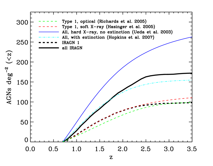
Figure 23.— Cumulative redshift distribution of IRAGNs, compared to predictions using optical and X-ray luminosity functions, and considering the Boötes flux limits. See text in § 7.5 for discussion.

7.5. Comparison to predictions from luminosity functions

Another check on the completeness of our selection is to compare the number of IRAGNs in our sample with the number that are predicted by optical, IR, and X-ray luminosity functions, accounting for the Boötes flux limits. Our AGN detection is usually limited by the 5.8 $\mu$m band (the 8 $\mu$m band has a similar flux limit, but since the quasars have red SEDs, they are usually brighter at 8 $\mu$m than at 5.8 $\mu$m). To convert X-ray and optical luminosities to IRAC fluxes, we use the AGN model (SDSS optical spectrum plus mid-IR power law) described in § 4.1. We include a distribution in IR slopes, modeled by a Gaussian with $\langle\alpha_{\nu}\rangle=-1$ and $\sigma_{\alpha_{\nu}}=0.5$. This distribution approximately reproduces the observed dispersion in the optical to IR colors for type 1 AGNs from Richards et al. (2006), as shown in Fig. 3.

We first compare the IRAGN 1 sample to the predictions of the broad-line quasar luminosity function of Richards et al. (2005) from the 2QZ survey. Unlike more recent luminosity functions derived from SDSS data, this data set includes objects below the “knee” of the luminosity function. This model SED, convolved with the Richards et al. (2005) luminosity function, predicts 840 type 1 quasars brighter than our flux limits in the 8.5 deg² field covered by IRAC (see the the green dashed line in Fig. 23). We detect 839 IRAGN 1s, very close to this total. This indicates that the IRAC color selection is highly complete for broad-line quasars (although some highly-reddened IRAGN 1s might not be included in the Richards et al. (2005) sample).

We also evaluate predictions for X-ray luminosity functions. We use the same model UV/IR spectrum described above, and take the relationship between UV luminosity and the UV/X-ray spectral slope $\alpha_{\rm ox}$ from Steffen et al. (2006). For simplicity, we assume a constant unabsorbed X-ray spectrum with $\Gamma=2$. The 0.5–2 keV luminosity function for unabsorbed (type 1) quasars of Hasinger et al. (2005) predicts 970 AGNs above our flux limits at $z>0.7$ (see the red dashed curve in Fig. 23), or 16% more than the number of IRAGN 1s.

In contrast, the 2–10 keV luminosity function of Ueda et al. (2003) predicts $\sim$2300 total AGNs, 55% more than we detect. However, although the Ueda et al. (2003) X-ray sample includes many AGNs that are X-ray absorbed, our model AGN SED used here does not include corresponding dust extinction. The solid blue line in Fig. 23 therefore represents the number of total AGNs that would be observed at the Boötes flux limits, in the absence of dust extinction.

The effects of dust extinction were included by Hopkins et al. (2007), who determined a parametrization of the bolometric luminosity function by fitting observed X-ray, optical, and IR luminosity functions. This work used the distribution in $N_{\rm H}$ observed by Ueda et al. (2003), and a typical Galactic gas-to-dust ratio, in predicting the numbers of observed AGNs. The total number of AGNs for the Boötes 4.5 $\mu$m flux limit is shown by the dot-dashed cyan line in Fig. 23. The model predicts 1320 detectable AGNs at $z>0.7$, 10% fewer than the total number of IRAGNs we observe.

We note that the Hopkins et al. (2007) predictions may provide only a lower limit on the number of detectable AGNs. If AGNs typically have a gas-to-dust ratio that is higher than the Galactic value (see § 5.2), this would tend to decrease the dust extinction for a given $N_{\rm H}$ distribution, and so would increase the number of detectable AGNs at a given flux limit. Still, the agreement between the observed number of IRAGN 1s and 2s and the predictions from luminosity functions indicates that our selection is reasonably complete to the flux limits of the survey. However, we are likely missing half or more of the total obscured AGN population because dust extinction causes them to fall below our IRAC flux limits or out of the S05 AGN color selection.

8. Discussion

8.1. Comparison to other obscured AGN samples

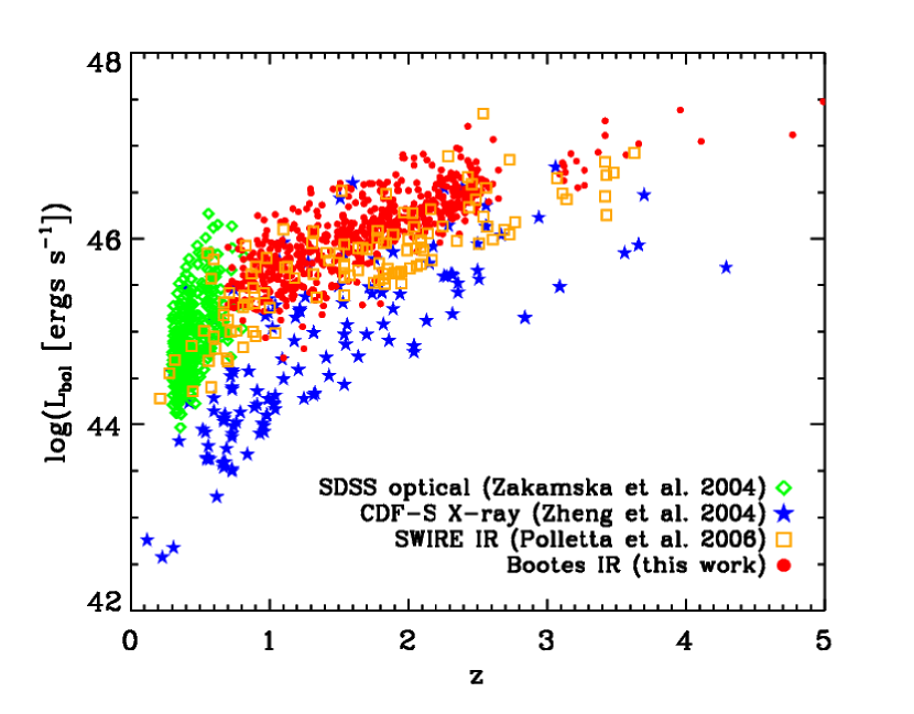
Figure 24.— $L_{\rm bol}$ versus redshift for four large samples of obscured AGNs: optically selected objects from SDSS (Zakamska et al., 2003, green triangles), X-ray selected objects from the CDF-S (Zheng et al., 2004, blue stars), IR-selected AGNs from the Chandra/SWIRE survey (Polletta et al., 2006, orange squares), and IRAGNs from this work (red circles). $L_{\rm bol}$ is estimated using bolometric corrections from Hopkins et al. (2007), as described in § 24.

In order to perform a complete census of obscured accretion in the Universe, it is important to place the IRAGN 2 sample described in this paper in the context of obscured AGNs found in other surveys. We compare the distribution in $z$ and $L_{\rm bol}$ of our sample with three of the largest ($>$100 objects) samples of obscured AGNs with redshift estimates.

The first sample consists of 291 optically-selected, luminous type 2 AGNs at $0.3<z<0.83$ from the SDSS (Zakamska et al., 2003). To estimate intrinsic $L_{\rm bol}$ from the observed spectroscopic properties, we assume that the unobscured SED of the type 2 quasars in this sample is similar to that for type 1 optical AGNs. In this case we use Equation (8) of Zakamska et al. (2003) to convert the observed [O III] $\lambda$5007 luminosity to the intrinsic, unobscured $L_{B}$. We then use the bolometric corrections from the model of Hopkins et al. (2007), for which $BC_{B}=9-12$.

The second sample consists of 145 X-ray sources in the CDF-S that are classified as type 2 AGNs on the basis of their X-ray spectrum and/or optical properties (Zheng et al., 2004). Of these objects, 68 have spectroscopic redshifts, while 78 have photo-$z$ estimates. For these objects we estimate an unabsorbed $L_{\rm 0.5-8\;keV}$ on the basis of the redshift, observed flux, and HR, assuming an intrinsic power-law spectrum with $\Gamma=1.8$. We then convert these values to $L_{\rm bol}$, again using the model of Hopkins et al. (2007), for which $BC_{\rm 0.5-8\;keV}\simeq 20-80$.

The third sample consists of the 120 obscured AGNs selected from optical and IR SEDs in the Chandra/SWIRE survey by Polletta et al. (2006). Of these objects, 11 have spectroscopic redshifts, and the remainder have photo-$z$’s. We calculate $L_{\rm bol}$ from the mid-IR luminosity $L_{\rm 4.5\mu m}$, as described in § 4.6. As a further check of the robustness of these $L_{\rm bol}$ estimates, we estimate $L_{\rm bol}$ for the 41 objects in the survey with X-ray detections, using the unabsorbed X-ray luminosities calculated by Polletta et al. (2006) and the Hopkins et al. (2007) SED model. We find that while there is significant scatter between the IR and X-ray estimates of $L_{\rm bol}$, on average they agree to within a factor of $\lesssim 2$. Nevertheless, these discrepancies between $L_{\rm bol}$ estimates require that our comparison between samples selected at different wavelengths is at best qualitative.

These samples of obscured AGNs selected in the optical (Zakamska et al., 2003), X-ray (Zheng et al., 2004), and IR (Polletta et al., 2006, this work) are shown in Fig. 24. The Boötes IRAGN 2s are more luminous than the X-ray selected AGNs from the CDF-S and at higher redshifts than those in the SDSS sample. The SWIRE obscured AGNs and Boötes IRAGN 2s have similar distributions in $z$ and $L_{\rm bol}$, but because of the much larger area in the Boötes field (8.5 deg² vs. 0.6 deg²), the Boötes IRAGN 2 sample contains $\sim$6 times more objects. We note that even accounting for possible 30% contamination (§ 7.3), the Boötes IRAGN 2s contain the largest sample to date of luminous, moderately obscured AGNs at high redshift.

8.2. Contribution to the cosmic X-ray background

Synthesis models require a population of obscured AGNs to produce the intensity and spectral shape of the CXB. From our stacking analysis, we estimate the contribution to the total CXB of the two IRAGN types defined in this paper. The extragalactic component of the CXB is well modeled by a power law with $\Gamma=1.4$ and normalization $10.9\pm 0.5$ photons cm^-1 s^-1 keV^-1 sr^-1 at 1 keV (e.g., Hickox & Markevitch, 2006; De Luca & Molendi, 2004). This gives CXB intensities of $7.6\times 10^{-12}$ ergs cm^-2 s^-1 deg^-2 in the 0.5–2 keV band and $1.5\times 10^{-11}$ ergs cm^-2 s^-1 deg^-2 in the 2–7 keV band.

Over the 2.9 deg² for which we perform the X-ray stacking analysis, the total fluxes listed in Table 2 correspond to intensities for the IRAGN 1s of $1.2\times 10^{-12}$ ergs cm^-2 s^-1 deg^-2 in the 0.5–2 keV band and $1.3\times 10^{-12}$ ergs cm^-2 s^-1 deg^-2 in the 2–7 keV band, which represent 16% and 9%, respectively, of the total CXB. For the IRAGN 2s the intensities are $3.0\times 10^{-13}$ ergs cm^-2 s^-1 deg^-2 in the 0.5–2 keV band and $6.0\times 10^{-13}$ ergs cm^-2 s^-1 deg^-2 in the 2–7 keV band, or 4% and 4% of the CXB, respectively. This indicates that selecting IR AGNs in shallow exposures and at $z>0.7$ only captures a small fraction of the sources that produce the X-ray background.

8.3. Implications of a bimodal distribution in obscuration

The bimodal distribution in $L_{R}/L_{\rm 4.5\mu m}$ (and accordingly $A_{V}$) observed in the IRAGNs may give clues to the distribution of material that obscures the central engine. A detailed comparison of the distribution of dust extinction to AGN obscuration models is beyond the scope of this paper, but we qualitatively consider two explanations for the bimodal extinction: a hard-edged torus, or obscuration as an evolutionary phase.

In the unified model, the obscuring material is in an extended distribution that surrounds the nucleus on scales of $\lesssim 100$ pc, possibly in the shape of a torus, such that the level of obscuration depends on the observer’s line of sight. These obscuring structures are well-established for local Seyfert galaxies (see Antonucci, 1993, and references therein), and there is evidence that they also exist in more distant, luminous quasars, for example from the detection of broad emission lines in polarized light that is scattered from the nucleus (Zakamska et al., 2005). In some models of the torus (e.g., Treister et al., 2004; Ibar & Lira, 2007), the obscuring medium is not homogeneous but varies in density with radius and angle from the axis of symmetry, so that there is a slow increase in obscuring column as the torus is seen more edge-on. However, this slow increase is inconsistent with the $A_{V}$ distribution we observe. Instead, a bimodal $A_{V}$ distribution could indicate an abrupt edge to the obscuring material rather than a smooth distribution and so provides a constraint on the obscuring geometry.

Alternatively, the obscuring material could be in the form of irregular clouds that surround the nucleus on scales as large as kiloparsecs. This material can be driven to the center of the galaxy by major galaxy mergers and can feed the AGNs (as well as nuclear starbursts) while also obscuring the central engine (e.g., Sanders et al., 1988; Hopkins et al., 2006b). In time, AGN winds may blow this material away from the nucleus, leading to an unobscured phase of AGN activity (e.g., Silk & Rees, 1998; Springel et al., 2005; Hopkins et al., 2006a). In this picture, obscured accretion is an evolutionary stage in the life of the quasar; as long as the blowout phase is short-lived, quasars will be seen with either significant or very little obscuration. Therefore, the bimodal distribution we observe may place constraints on the timescale for AGN feedback.

9. Summary

In this paper we analyze a sample of 1479 AGNs at $0.7<z\lesssim 3$ from the wide-field multiwavelength Boötes survey, selected on the basis of their IRAC colors. This work has two key elements that together make it unique among studies of IR-selected AGN: (1) the wide area and deep optical photometry in the Boötes field allow us to identify a large number of obscured sources, and (2) the contiguous X-ray coverage allows us to verify independently that the IRAGN 2s are obscured AGNs, and to measure their neutral gas column densities.

Key results of this paper are as follows:

1. The optical-IR color distribution of the IR-selected AGNs is bimodal, with a boundary of $R-[4.5]=6.1$ (Vega) between the two subsets. Based on this color criterion, we divide our sample into 640 obscured (IRAGN 2) and 839 unobscured (IRAGN 1) AGNs. The optical-IR color distribution can be interpreted in terms of dust extinction of the nuclear optical emission for the IRAGN 2s. The obscured AGN color selection is valid for AGNs at $z>0.7$ and with mid-IR luminosities $\gtrsim 10^{11}$ $L_{\sun}$.

2. X-ray and optical data confirm our selection of obscured AGNs. X-ray stacking shows that both subsets of IRAGNs have average X-ray luminosities characteristic of luminous AGNs. The IRAGN 1s have average X-ray hardness ratios typical of unobscured sources, while the IRAGN 2s have harder X-ray spectra, corresponding to absorption with typical $N_{\rm H}\sim 3\times 10^{22}$ cm^-2. The optical colors and morphologies are typical of galaxies for most IRAGN 2s and of quasars for most IRAGN 1s, consistent with the optical emission from the IRAGN 2s being extincted.

3. For a typical range of AGN gas-to-dust ratios, the $N_{\rm H}$ for the IRAGN 2s (derived from X-ray stacking) corresponds to $1\lesssim A_{V}\lesssim 10$, consistent with the $A_{V}$ values derived from optical-IR SED fits, and sufficient to completely extinct the nuclear optical emission. This indicates that, on average, absorption by neutral gas and extinction by dust are correlated in these luminous AGNs.

4. The S05 IRAC color-color AGN selection is reasonably complete to our survey flux limits. The numbers of IRAGN 1s and 2s are within $\sim$15% of predictions from optical and X-ray luminosity functions. We expect the optical/IR color selection to be at least 80% reliable in distinguishing between unobscured and obscured AGNs, while contamination from starburst galaxies in the IRAGN 2 sample should be at most $\sim$30% and is likely much lower.

5. The bimodal distribution in optical-IR color for IRAGNs suggests that these objects have either low ($A_{V}\lesssim 0.1$) or significant ($A_{V}\gtrsim 0.7$) extinction. This distribution may have implications for models of AGN obscuration. In the context of the unified model, this may imply a hard edge to distribution of obscuring material. Alternatively, obscuration may be an evolutionary phase that is followed by rapid blowout of the obscuring dust, leading to a bimodal distribution in $A_{V}$.

6. The IRAGN 2s comprise the largest sample to date of AGNs with high redshifts ($0.7<z<3$), high bolometric luminosities ($10^{45}\lesssim L_{\rm bol}\lesssim 10^{47}$ ergs s^-1), and moderate absorption ($10^{22}\lesssim N_{\rm H}\lesssim 10^{23}$ cm^-2), even after accounting for possible sample contamination of at most $\sim$30%. This work shows that IRAC and optical selection is a powerful tool for identifying large numbers of luminous, obscured AGNs for follow-up study.

References

- Akylas et al. (2006) Akylas, A., Georgantopoulos, I., Georgakakis, A., Kitsionas, S., & Hatziminaoglou, E. 2006, A&A, 459, 693
- Alexander et al. (2005) Alexander, D. M., Bauer, F. E., Chapman, S. C., Smail, I., Blain, A. W., Brandt, W. N., & Ivison, R. J. 2005, ApJ, 632, 736
- Alonso-Herrero et al. (2006) Alonso-Herrero, A., et al. 2006, ApJ, 640, 167
- Antonucci (1993) Antonucci, R. 1993, ARA&A, 31, 473
- Awaki et al. (1991) Awaki, H., Koyama, K., Inoue, H., & Halpern, J. P. 1991, PASJ, 43, 195
- Ballantyne et al. (2006) Ballantyne, D. R., Shi, Y., Rieke, G. H., Donley, J. L., Papovich, C., & Rigby, J. R. 2006, ApJ, 653, 1070
- Barger et al. (2005) Barger, A. J., Cowie, L. L., Mushotzky, R. F., Yang, Y., Wang, W.-H., Steffen, A. T., & Capak, P. 2005, AJ, 129, 578
- Barmby et al. (2006) Barmby, P., et al. 2006, ApJ, 642, 126
- Becker et al. (2007) Becker, G. D., Rauch, M., & Sargent, W. L. W. 2007, ApJ, 662, 72
- Becker et al. (1995) Becker, R. H., White, R. L., & Helfand, D. J. 1995, ApJ, 450, 559
- Bertin & Arnouts (1996) Bertin, E. & Arnouts, S. 1996, A&AS, 117, 393
- Best et al. (2005) Best, P. N., Kauffmann, G., Heckman, T. M., Brinchmann, J., Charlot, S., Ivezić, Ž., & White, S. D. M. 2005, MNRAS, 362, 25
- Bolzonella et al. (2000) Bolzonella, M., Miralles, J.-M., & Pelló, R. 2000, A&A, 363, 476
- Brand et al. (2006) Brand, K., et al. 2006, ApJ, 641, 140
- Brand et al. (2005) Brand, K., et al. 2005, ApJ, 626, 723
- Brand et al. (2007) Brand, K., et al. 2007, ApJ in press (arXiv:0709.3119), 709
- Brandt & Hasinger (2005) Brandt, W. N. & Hasinger, G. 2005, ARA&A, 43, 827
- Brodwin et al. (2006) Brodwin, M., et al. 2006, ApJ, 651, 791
- Brown et al. (2006) Brown, M. J. I., et al. 2006, ApJ, 638, 88
- Buchanan et al. (2006) Buchanan, C. L., Gallimore, J. F., O’Dea, C. P., Baum, S. A., Axon, D. J., Robinson, A., Elitzur, M., & Elvis, M. 2006, AJ, 132, 401
- Caccianiga et al. (2004) Caccianiga, A., et al. 2004, A&A, 416, 901
- Comastri et al. (1995) Comastri, A., Setti, G., Zamorani, G., & Hasinger, G. 1995, A&A, 296, 1
- Cutri et al. (2002) Cutri, R. M., Nelson, B. O., Francis, P. J., & Smith, P. S. 2002, in ASP Conf. Ser. 284: IAU Colloq. 184: AGN Surveys, ed. R. F. Green, E. Y. Khachikian, & D. B. Sanders (San Francisco: ASP), 127
- Daddi et al. (2007) Daddi, E., et al. 2007, ApJ in press, astro-ph/0705.2832
- De Luca & Molendi (2004) De Luca, A. & Molendi, S. 2004, A&A, 419, 837
- Dwelly & Page (2006) Dwelly, T. & Page, M. J. 2006, MNRAS, 372, 1755
- Dwelly et al. (2005) Dwelly, T., Page, M. J., Loaring, N. S., Mason, K. O., McHardy, I., Gunn, K., & Sasseen, T. 2005, MNRAS, 360, 1426
- Eisenhardt et al. (2004) Eisenhardt, P. R., et al. 2004, ApJS, 154, 48
- Fall & Pei (1989) Fall, S. M. & Pei, Y. C. 1989, ApJ, 337, 7
- Farrah et al. (2003) Farrah, D., Afonso, J., Efstathiou, A., Rowan-Robinson, M., Fox, M., & Clements, D. 2003, MNRAS, 343, 585
- Farrah et al. (2002) Farrah, D., Serjeant, S., Efstathiou, A., Rowan-Robinson, M., & Verma, A. 2002, MNRAS, 335, 1163
- Fioc & Rocca-Volmerange (1997) Fioc, M. & Rocca-Volmerange, B. 1997, A&A, 326, 950
- Gehrels (1986) Gehrels, N. 1986, ApJ, 303, 336
- Gilli et al. (2007) Gilli, R., Comastri, A., & Hasinger, G. 2007, A&A, 463, 79
- Glikman et al. (2006) Glikman, E., Helfand, D. J., & White, R. L. 2006, ApJ, 640, 579
- Gorjian et al. (2007) Gorjian, V., et al. 2007, submitted to ApJ
- Guainazzi et al. (2005) Guainazzi, M., Matt, G., & Perola, G. C. 2005, A&A, 444, 119
- Hao et al. (2005) Hao, L., et al. 2005, AJ, 129, 1795
- Hasinger et al. (2005) Hasinger, G., Miyaji, T., & Schmidt, M. 2005, A&A, 441, 417
- Hatziminaoglou et al. (2005) Hatziminaoglou, E., et al. 2005, AJ, 129, 1198
- Helou et al. (1985) Helou, G., Soifer, B. T., & Rowan-Robinson, M. 1985, ApJ, 298, L7
- Hickox & Markevitch (2006) Hickox, R. C. & Markevitch, M. 2006, ApJ, 645, 95
- Ho (2005) Ho, L. C. 2005, astro-ph/0511157
- Hogg (1999) Hogg, D. W. 1999, astro-ph/9905116
- Hopkins et al. (2006a) Hopkins, P. F., Hernquist, L., Cox, T. J., Di Matteo, T., Robertson, B., & Springel, V. 2006a, ApJS, 163, 1
- Hopkins et al. (2007) Hopkins, P. F., Richards, G. T., & Hernquist, L. 2007, ApJ, 654, 731
- Hopkins et al. (2006b) Hopkins, P. F., Somerville, R. S., Hernquist, L., Cox, T. J., Robertson, B., & Li, Y. 2006b, ApJ, 652, 864
- Houck et al. (2005) Houck, J. R., et al. 2005, ApJ, 622, L105
- Ibar & Lira (2007) Ibar, E. & Lira, P. 2007, A&A, 466, 531
- Indebetouw et al. (2005) Indebetouw, R., et al. 2005, ApJ, 619, 931
- Jannuzi & Dey (1999) Jannuzi, B. T. & Dey, A. 1999, in Astronomical Society of the Pacific Conference Series, Vol. 191, Photometric Redshifts and the Detection of High Redshift Galaxies, ed. R. Weymann, L. Storrie-Lombardi, M. Sawicki, & R. Brunner (San Francisco: ASP), 111
- Kenter et al. (2005) Kenter, A., et al. 2005, ApJS, 161, 9
- Khachikian & Weedman (1974) Khachikian, E. Y. & Weedman, D. W. 1974, ApJ, 192, 581
- King (2005) King, A. 2005, ApJ, 635, L121
- La Franca et al. (2005) La Franca, F., et al. 2005, ApJ, 635, 864
- Lacy et al. (2007) Lacy, M., Petric, A. O., Sajina, A., Canalizo, G., Storrie-Lombardi, L. J., Armus, L., Fadda, D., & Marleau, F. R. 2007, AJ, 133, 186
- Lacy et al. (2004) Lacy, M., et al. 2004, ApJS, 154, 166
- Lawrence (1991) Lawrence, A. 1991, MNRAS, 252, 586
- Maiolino & Rieke (1995) Maiolino, R. & Rieke, G. H. 1995, ApJ, 454, 95
- Martínez-Sansigre et al. (2006) Martínez-Sansigre, A., Rawlings, S., Lacy, M., Fadda, D., Jarvis, M. J., Marleau, F. R., Simpson, C., & Willott, C. J. 2006, MNRAS, 370, 1479
- Mateos et al. (2005) Mateos, S., Barcons, X., Carrera, F. J., Ceballos, M. T., Hasinger, G., Lehmann, I., Fabian, A. C., & Streblyanska, A. 2005, A&A, 444, 79
- Matt (2002) Matt, G. 2002, in ASP Conf. Ser. 258: Issues in Unification of Active Galactic Nuclei, ed. R. Maiolino, A. Marconi, & N. Nagar (San Francisco: ASP), 3
- McCarthy (1993) McCarthy, P. J. 1993, ARA&A, 31, 639
- Murray et al. (2005) Murray, S. S., et al. 2005, ApJS, 161, 1
- Mushotzky (2004) Mushotzky, R. 2004, in Astrophysics and Space Science Library, Vol. 308, Supermassive Black Holes in the Distant Universe, ed. A. J. Barger (Dordrecht: Kluwer), 53
- Narayan & Yi (1995) Narayan, R. & Yi, I. 1995, ApJ, 452, 710
- Osterbrock & Shaw (1988) Osterbrock, D. E. & Shaw, R. A. 1988, ApJ, 327, 89
- Pei (1992) Pei, Y. C. 1992, ApJ, 395, 130
- Polletta et al. (2006) Polletta, M. d. C., et al. 2006, ApJ, 642, 673
- Puget & Leger (1989) Puget, J. L. & Leger, A. 1989, ARA&A, 27, 161
- Ranalli et al. (2003) Ranalli, P., Comastri, A., & Setti, G. 2003, A&A, 399, 39
- Richards et al. (2005) Richards, G. T., et al. 2005, MNRAS, 360, 839
- Richards et al. (2006) Richards, G. T., et al. 2006, ApJS, 166, 470
- Rowan-Robinson et al. (2005) Rowan-Robinson, M., et al. 2005, AJ, 129, 1183
- Sanders et al. (1988) Sanders, D. B., Soifer, B. T., Elias, J. H., Madore, B. F., Matthews, K., Neugebauer, G., & Scoville, N. Z. 1988, ApJ, 325, 74
- Setti & Woltjer (1989) Setti, G. & Woltjer, L. 1989, A&A, 224, L21
- Seyfert (1943) Seyfert, C. K. 1943, ApJ, 97, 28
- Siebenmorgen & Krügel (2007) Siebenmorgen, R. & Krügel, E. 2007, A&A, 461, 445
- Silk & Rees (1998) Silk, J. & Rees, M. J. 1998, A&A, 331, L1
- Spoon et al. (2005) Spoon, H. W. W., et al. 2005, in IAU Symposium, ed. D. C. Lis, G. A. Blake, & E. Herbst (Cambridge: Cambridge University Press), 281–290
- Springel et al. (2005) Springel, V., Di Matteo, T., & Hernquist, L. 2005, MNRAS, 361, 776
- Steffen et al. (2006) Steffen, A. T., Strateva, I., Brandt, W. N., Alexander, D. M., Koekemoer, A. M., Lehmer, B. D., Schneider, D. P., & Vignali, C. 2006, AJ, 131, 2826
- Stern et al. (2005) Stern, D., et al. 2005, ApJ, 631, 163
- Stern et al. (2002) Stern, D., et al. 2002, ApJ, 568, 71
- Sturm et al. (2006) Sturm, E., Hasinger, G., Lehmann, I., Mainieri, V., Genzel, R., Lehnert, M. D., Lutz, D., & Tacconi, L. J. 2006, ApJ, 642, 81
- Tozzi et al. (2006) Tozzi, P., et al. 2006, A&A, 451, 457
- Treister & Urry (2005) Treister, E. & Urry, C. M. 2005, ApJ, 630, 115
- Treister et al. (2004) Treister, E., et al. 2004, ApJ, 616, 123
- Ueda et al. (2003) Ueda, Y., Akiyama, M., Ohta, K., & Miyaji, T. 2003, ApJ, 598, 886
- Urry & Padovani (1995) Urry, C. M. & Padovani, P. 1995, PASP, 107, 803
- van Breugel et al. (1999) van Breugel, W., De Breuck, C., Stanford, S. A., Stern, D., Röttgering, H., & Miley, G. 1999, ApJ, 518, L61
- Vanden Berk et al. (2001) Vanden Berk, D. E., et al. 2001, AJ, 122, 549
- Webster et al. (1995) Webster, R. L., Francis, P. J., Peterson, B. A., Drinkwater, M. J., & Masci, F. J. 1995, Nature, 375, 469
- Weedman et al. (2006) Weedman, D., et al. 2006, ApJ, 653, 101
- Wilkes et al. (2002) Wilkes, B. J., Schmidt, G. D., Cutri, R. M., Ghosh, H., Hines, D. C., Nelson, B., & Smith, P. S. 2002, ApJ, 564, L65
- Zakamska et al. (2005) Zakamska, N. L., et al. 2005, AJ, 129, 1212
- Zakamska et al. (2004) Zakamska, N. L., Strauss, M. A., Heckman, T. M., Ivezić, Ž., & Krolik, J. H. 2004, AJ, 128, 1002
- Zakamska et al. (2003) Zakamska, N. L., et al. 2003, AJ, 126, 2125
- Zheng et al. (2004) Zheng, W., et al. 2004, ApJS, 155, 73