Memory Effect and Fast Spinodal Decomposition

Abstract

We consider the modification of the Cahn-Hilliard equation when a time delay process through a memory function is taken into account. We then study the process of spinodal decomposition in fast phase transitions associated with a conserved order parameter. The introduced memory effect plays an important role to obtain a finite group velocity. Then, we discuss the constraint for the parameters to satisfy causality. The memory effect is seen to affect the dynamics of phase transition at short times and has the effect of delaying, in a significant way, the process of rapid growth of the order parameter that follows a quench into the spinodal region.

Keywords: Non-equilibrium field dynamics; Memory effects; Relativistic heavy-ion collisions

I Background

Diffusion is a typical relaxation process and appears in various fields of physics: thermal diffusion processes, spin diffusion processes, Brownian motions and so on. It is empirically known that the dynamics of these processes is approximately given by the diffusion equation. Although the diffusion equation has broad applicability, there exist the applicability limitations. First, the diffusion equation does not obey causalityref:1 . Let us consider the following telegraph equation,

$$\tau\frac{d^{2}}{dt^{2}}m(x,t)+\frac{d}{dt}n(x,t)-D\nabla^{2}n(x,t)=0.$$ (1)

Then, the propagation speed is given by $v=\sqrt{D/\tau}$. Thus, the propagation speed of the diffusion equation is infinite because the telegraph equation is reduced to the diffusion equation in the limit of vanishing $\tau$. Second, the diffusion equation does not satisfy exact relations, for instance, the Kramers-Kronig relation and the f-sum rule ref:Kada-M ; ref:Koide . By solving the Heisenberg equation of motion, the exact Laplace-Fourier transform of the time-evolution of a conserved number density is given by

$$\delta n^{LF}(k,z)=\frac{i}{z}C(k)+\frac{i}{z^{3}}\frac{k^{2}}{m}\langle n(0)\rangle_{eq}+{\cal O}(1/z^{4}),$$ (2)

where $\delta$ means the fluctuations from the equilibrium value and $C(k)$ represents the Fourier transform of the correlation function of the number density. Because of the Kramers-Kronig relation and the f-sum rule, the term proportional to $1/z^{2}$ disappears and the coefficient of the second term is proportional to the equilibrium expectation value of the total number $\langle n(0)\rangle_{eq}$. These are not satisfied if the coarse-grained dynamics of the number density is assumed to be given by the diffusion equation ref:Kada-M ; ref:Koide .

It is known that the problem of causality and the sum rules can be solved by using the telegraph equation instead of the diffusion equation. Interestingly enough, it has been shown recently that the coarse-grained equation derived by employing systematic coarse-grainings from the Heisenberg equation of motion is not the diffusion equation but the telegraph equation ref:Koide ; ref:footnote1 .

The discussion so far is applicable to conserved quantities because the diffusion equation is a coarse-grained equation of conserved quantities. On the other hand, the corresponding equation for a non-conserved quantity is the time-dependent Ginzburg-Landau (TDGL) equation in the sense that the TDGL equation is a overdamping equation. The microscopic calculation ref:Koide-M again shows that the relaxation phenomenon is accompanied by oscillation and cannot be described by the TDGL equation as is the case with conserved quantities. As a matter of fact, the equation has a similar form to the telegraph equation.

The effect discussed above is, in particular, important for fast processes where the time scale of memory is not short enough, because the telegraph equation can be obtained by introducing the memory effect to the diffusion equation. Such fast phase transitions are expected to have happened in early universe and most certainly also characterize the phase transitions expected to occur in the highly excited matter created in relativistic heavy-ion collisions. In the early universe, such situations may have happened when the typical microscopic time scales for relaxation, given by the inverse of the decay width associated with particle dynamics, is larger than the Hubble time. This is a situation likely to be expected when describing GUT phase transitions or even the inflationary dynamics ref:Rudnei . In relativistic heavy-ion collisions, one expected to learn about the QCD phase transition. For instance, from the hydrodynamic analysis of the freeze-out temperature in the most central Au-Au collisions at 130 A GeV, the typical reaction time is given by around 10-20 fm ref:Hama . However, the characteristic time scale of the memory function in the Langevin equation which describes the dynamics of the order parameter of the chiral phase transition is predicted to be about 1 fm, which is not enough short to be ignored ref:Koide-M .

II Memory effect in spinodal decomposition

So far, we have discussed the difficulties with causality and memory effects, and sum rules associated with linear processes. Next, we consider such problems associated with a nonlinear process, known as spinodal decomposition(SD) ref:KGR .

We consider the general Ginzburg-Landau (GL) Free energy,

$$F(\phi)=\int d^{3}{\bf x}\left[\frac{a}{2}(\nabla\phi)^{2}-\frac{b}{2}\phi^{2}+\frac{c}{4}\phi^{4}\right],$$ (3)

where $\phi$ is a conserved order parameter. To describe the phase transition, the parameter $b$ is proportional to $T_{c}-T$ with $T_{c}$ being the critical temperature of the associated second order phase transition. The dynamics of conserved order parameters can be described by the Cahn-Hilliard (CH) equation. In the ordinary CH equation, the irreversible current induced by the GL free energy is given by

$${\bf J}(x,t)=-\Gamma\nabla\frac{\delta F(\phi)}{\delta\phi},$$ (4)

where $\Gamma$ denotes a kind of Onsager coefficient. To take the memory effect into account, the current is generalized as follows,

$${\bf J}(x,t)=-\int^{t}_{0}dsd^{3}{\bf x}^{\prime}{\cal M}({\bf x-x^{\prime}},t-s)\nabla_{\bf x^{\prime}}\frac{\delta F(\phi)}{\delta\phi({\bf x}^{\prime},s)}.$$ (5)

For simplicity, we assume the following memory function,

$${\cal M}(x,t)=\frac{\Gamma}{\gamma}e^{-t/\gamma}\delta^{(3)}(x).$$ (6)

Here, the typical memory time is characterized by $\gamma$. Substituting the current to the equation of continuity, we obtain the modified CH equation,

$$\gamma\frac{\partial^{2}}{\partial t^{2}}\phi(x,t)+\frac{\partial}{\partial t}\phi(x,t)=\Gamma\nabla^{2}\frac{\delta F(\phi)}{\delta\phi}.$$ (7)

At the late stage of the spinodal decomposition, the behavior of the process is described by the linearized equation around equilibrium order parameter $\phi_{0}=\sqrt{b/a}$,

$$\gamma\frac{\partial^{2}}{\partial t^{2}}\tilde{\phi}_{c}(k,t)+\frac{\partial}{\partial t}\tilde{\phi}_{c}(k,t)=-\Gamma k^{2}(ak^{2}+2b)\tilde{\phi}_{c}(k,t),$$ (8)

whose solution is $\tilde{\phi}_{c}(k,t)=A_{k}\exp(\lambda_{+}^{\prime}t)+B_{k}\exp(\lambda_{-}^{\prime}t)$, where $A_{k}$ and $B_{k}$ are arbitrary constants and

$$\lambda_{\pm}^{\prime}=\frac{-1\pm\sqrt{1-4\gamma\Gamma k^{2}(ak^{2}+2b)}}{2\gamma}.$$ (9)

On the other hand, the solution for the corresponding ordinary CH equation ($\gamma=0$) is $\tilde{\phi}_{nc}(k,t)=C_{k}\exp[-\Gamma k^{2}(2b+ak^{2})t]$. One can easily see that there exists a critical momentum for the solution of the modified CH equation, ${k^{\prime}}^{2}_{c}=[-b+\sqrt{b^{2}+a/(4\gamma\Gamma)}]/a$. Below the critical momentum, the solution shows overdamping behavior similar to the ordinary CH solution, while above the critical momentum, the damping is accompanied by the oscillatory fluctuation mode. Thus, we can consider that the critical momentum is a kind of a ultraviolet cutoff because the higher momentum modes have rapid oscillations and cancel in computing averages. The propagation speed is characterized by the group velocity. In the modified CH equation, this is given by

$$v(k)=\frac{\sqrt{2D}(\xi^{2}k^{2}+1)}{\sqrt{\gamma(\xi^{2}k^{2}+2)}},$$ (10)

where $D=2b\Gamma$ and $\xi=\sqrt{a/b}$. At $k=0$, the group velocity reads $v(0)=\sqrt{D/\gamma}$. The maximum group velocity is a monotonically increase function of $k$. Because of the momentum cutoff discussed above, the maximum group velocity is given by

$$v(k^{\prime}_{c})=\frac{2D}{\gamma}\frac{1+\xi^{2}/(2\gamma D)}{1+\sqrt{1+\xi^{2}/(2\gamma D)}}.$$ (11)

For causality, Eq. (11) should be less than one. This leads to the constraint $\gamma>D$. In other words, we can always find allowed values of parameters for which the spinodal decomposition is causal, under the constraint. In Fig. 1, the group velocity is plotted as function of $D$ for a fixed value $\xi=1$. The three lines corresponds to $\gamma=D$, $D+0.1$ and $D+1$, respectively. One can see that the group velocity is larger than one for any $D$ at $\gamma=D$. At $\gamma=D+0.1$, one can find $D$ where the group velocity is less than one. At $\gamma=D+1$, the group velocity is less than one for any $D$. The modified CH equation satisfies causality in this sense.

Figure 1: The group velocity (11) as function of $D$ for a fixed value $\xi=1$. The three lines are corresponding to $\gamma=D$, $D+0.1$ and $D+1$, respectively.

Let us see how this also applies for instance to the spinodal modes and then use these results e.g. for the problem of searching a signal of a phase transition in RHIC. By considering the fastest-growing mode of the SD, which is defined by

$$\left.\frac{\partial}{\partial k}\frac{-1+\lambda}{2\gamma}\right|_{k_{r}}=0,$$ (12)

we derive the time scale of the fastest mode to be

$$\tau_{c}(k_{r})=\frac{2\gamma}{-1+\sqrt{1+\gamma D/(2\xi^{2})}}.$$ (13)

When $\gamma$ is very small, the time scale is reduced to $\tau_{nc}(k_{r})=8\xi^{2}/D$, which agrees with the time scale of the SD without the effect of memory ref:gavin2 . Since the modes that give the result of Eq. (13) are in fact the dominant spinodal modes and $\tau_{nc}<\tau_{c}$, this reflects itself in an overall delay of the time formation of domains, as described by the causal CH equation compared to the noncausal one, as the phase transition proceeds. This feature is confirmed by our simulations shown below. For a problem like RHIC and a possible signature of a phase transition coming from it, this difference in time scales can be very pronounced and lead to a striking effect that a signal, like charge fluctuations and domain formation, can be so much delayed that possibly could not be observed in the current experiments. For instance, in RHIC, the correlation length is typically $\xi\sim 1$ fm. Using also the relation between the parameters $D$ and $\gamma$ obtained for a quark plasma, $\gamma=3D$, which is consistent with our constraint condition obtained from Eq. (11), and considering $D\sim 3.7$ fm ref:gavin2 ; ref:gavin , we obtain from Eq. (13) that $\tau_{c}\sim 6.1$ fm, which is to be compared with the result $\tau_{nc}\sim 2.2$ fm. This represents almost a $200\%$ difference for the time scales for the starting of the growth of fluctuations in Eq. (7) as compared to the ordinary CH equation (for $\gamma=0$).

We have solved Eq. (7) numerically on a discrete spatial square lattice using a semi-implicit scheme in time, with a fast Fourier transform in the spatial coordinates ref:KGR . We have checked the stability of the results by changing lattice spacings and time steps. In addition, for $\gamma>1$ we have also used a leap-frog algorithm and the results obtained with both methods agreed very well. For the noncausal $\gamma=0$ equation, we used as initial condition $\phi({\bf x},t=0)$ a random distribution in space with zero average and amplitude $10^{-3}$. For $\gamma\neq 0$, we used in addition the condition that at $t=0$ the first-order derivative of $\phi$ is zero. For the numerical work, Eq. (7) is re-parameterized to dimensionless variables, conveniently defined by time $\bar{t}=(8/\tau_{nc})t=(2b^{2}\Gamma/a)t$, space coordinates $\bar{x}_{i}=x_{i}/\xi$, field $\bar{\phi}=\sqrt{c/b}\,\phi$ and $\bar{\gamma}=(8/\tau_{nc})\gamma$. In terms of these variables Eq. (7) becomes function of only one parameter, $\bar{\gamma}$. Eq. (7) was next solved for several values of $\bar{\gamma}$. Two representatives results, for $\bar{\gamma}=0$ and $\bar{\gamma}=40.5$ (for the example analyzed in the previous paragraph), are shown in Fig. 2.

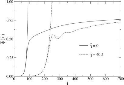
Figure 2: Volume average of $\bar{\phi}(\bar{t})$ as a function of dimensionless time $\bar{t}$ for the noncausal (solid) and causal (dashed) solutions. The two curves that exit the top of the plot are results from the linearized theory.

In Fig. 2 we present the time evolution of the volume average of the order parameter $\phi$, defined as $\bar{\phi}(t)=\frac{1}{N^{3}}\sum_{{\bf x}}\langle\bar{\phi}({\bf x},t)_{+}\rangle$, where $N^{3}$ is the total number of lattice points and the average is taken over different initial random configurations. $\phi({\bf x},t)_{+}$ indicates that only the positive values of the field are considered (i.e., a specific direction for the field has been selected). The rapid increase of $\bar{\phi}$ reflects the phenomenon of SD. The figure also shows the results by solving the linear equation. It shows that it performs extremely well up to and right after the spinodal growth of the order parameter, then justifying our previous analytical results based on the solution of the linear equation. The effect of $\gamma$ is seen to be more important at earlier times, consistent with the memory function used and becomes less important after the rapid growth of the order parameter (the spinodal explosion). It also shows the effect of a finite $\gamma$, increasing dramatically the delay of the spinodal explosion, as predicted by our previous analytical results. The time for reaching equilibrium is seen to be very long, as is common with the traditional noncausal CH equation. Also apparent from Fig. 2 are the oscillations in the order parameter for a finite $\gamma$, also predicted by our previous analysis. This is due to the increasing importance of the second-order time derivative as compared to the first-order one as $\gamma$ increases, i.e. as $\gamma$ increases the dissipation term becomes less important and the equation becomes more and more a wave-like equation. The estimated delay for the thermalization is even larger than the recent estimation ref:FK for the time delay of the relaxation of a nonconserved order parameter.

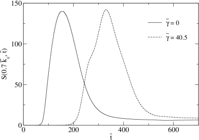
Figure 3: Spherically averaged structure function as a function of dimensionless time $\bar{t}$ for a $\bar{k}=0.7\bar{k}_{c}$ for the noncausal (solid) and causal (dashed) solutions.

We have also investigated the effect of memory for the structure function, $S(k,t)=|\phi({\bf k},t)|^{2}$. This quantity is important because it provides information on the space-time coarsening of the domains of the different phases. In Fig. 3 we present the results for the spherically averaged value of $S$ for $k=0.7k_{c}$ (to emphasize the fast growth of the long wavelength fluctuations with $k<k_{c}$). The spherical averaging for a given $k$ was done over momenta $k_{r}=\sqrt{k^{2}_{x}+k^{2}_{y}+k^{2}_{z}}$ such that $k-0.1\Delta\leq k_{r}\leq k+0.1\Delta$, with $\Delta=2\pi/L$, where $L$ is the size of the lattice. Consistently with Fig. 2, this figure shows the dramatic delay for the spinodal growth.

III conclusion

We have introduced memory effects into the CH equation. By introducing the memory effects, we could define the group velocity and, to satisfy causality, we were able derive the constraint for the parameters of the CH equation. For a physical situation of interest for the phenomenology of RHIC, we found that the inclusion of memory effects can delay substantially the phase-separation process and consequently, there might not be enough time for the system to thermalize before the breakdown of the system due to expansion.

In this paper, we simply discussed the case of memory function which has the exponential form. However, we can generalize the present work by considering other types of memory functions. In particular, microscopic calculations from nonequilibrium quantum field theory ref:Rudnei show that memory functions tend to exhibit relaxation as well oscillations as time goes on. Then, we can consider the following physically motivated from those field theory calculations,

$${\cal M}({\bf x},t)=\frac{\Gamma}{\gamma}\,e^{-t/\gamma}\cos(\Omega t)\delta^{(3)}({\bf x}),$$ (14)

where $\Omega$ is some characteristic frequency of oscillation. Substituting (14) into the equation of continuity, we obtain

$$\gamma^{2}\frac{\partial^{3}}{\partial t^{3}}\phi({\bf x},t)+2\gamma\frac{\partial^{2}}{\partial t^{2}}\phi({\bf x},t)+(1+\gamma^{2}\Omega^{2})\frac{\partial}{\partial t}\phi({\bf x},t)$$

$$=\Gamma\,\nabla^{2}\frac{\delta F(\phi)}{\delta\phi}+\gamma\Gamma\frac{\partial}{\partial t}\,\nabla^{2}\frac{\delta F(\phi)}{\delta\phi}.$$ (15)

This result and the example worked out explicitly in this work shows that the macroscopic dynamics of conserved quantities strongly depends on the choice of the memory function. In these cases, the use of microscopic motivated memory functions based on the particular model under study is fundamental. An analysis for (15), analogous to the one performed in this work for the simplest exponential decay memory function, will be presented elsewhere.

- (1) D. Jou, J. Casas-Vázquez and G. Leben, Rep. Prog. Phys. 51, 1105 (1988); ibid. 62, 1035 (1999).
- (2) L. P. Kadanoff and P. C. Martin, Ann. Phys. (N.Y.) 24, 419 (1963).
- (3) T. Koide, Phys. Rev. E72, 026135 (2005).
- (4) This microscopic calculation further makes it appear that the relaxation time contained in the telegraph equation is not constant and has momentum dependence.
- (5) T. Koide and M. Maruyama, Nucl. Phys. A742, 95 (2004).
- (6) M. Gleiser and R. O. Ramos, Phys. Rev. D50, 2441 (1994); A. Berera and R. O. Ramos, Phys. Rev. D63, 103509 (2001); Phys. Lett. B607, 1 (2005); Phys. Rev. D71, 023513 (2005).
- (7) Y. Hama, T. Kodama and O. Socolowski Jr., Braz. J. Phys. 35, 24 (2005).
- (8) T. Koide,G. Krein and R. O. Ramos, Phys. Lett. B 636, 96 (2006).
- (9) D. Bower and S. Gavin, Phys. Rev. C 64, 051902 (2001)
- (10) M. A. Aziz and S. Gavin, Phys. Rev. C 70, 034905 (2004).
- (11) E. S. Fraga and G. Krein, Phys. Lett. B614, 181 (2005).