Rate of Escape on the Lamplighter Tree

Abstract.

Suppose we are given a homogeneous tree $\mathcal{T}_{q}$ of degree $q\geq 3$, where at each vertex sits a lamp, which can be switched on or off. This structure can be described by the wreath product $(\mathbb{Z}/2)\wr\Gamma$, where $\Gamma=\ast_{i=1}^{q}\mathbb{Z}/2$ is the free product group of $q$ factors $\mathbb{Z}/2$. We consider a transient random walk on a Cayley graph of $(\mathbb{Z}/2)\wr\Gamma$, for which we want to compute lower and upper bounds for the rate of escape, that is, the speed at which the random walk flees to infinity.

Lorenz A. Gilch

Graz University of Technology, Graz, Austria

1. Introduction

Consider a homogeneous tree $\mathcal{T}_{q}$ of degree $q\geq 3$, where a lamp sits at each vertex, which can have the states 0 (“off”) or 1 (“on”). Initially, all lamps are off. We think of a lamplighter walking randomly along the tree and switching lamps on or off. Whenever he stands at a vertex of $\mathcal{T}_{q}$ he tosses a coin and decides to change the lamp state at his actual position or to travel to a random neighbour vertex. This is modeled by a transient Markov chain $(Z_{n})_{n\geq 0}$, which represents the position of the lamplighter and the lamp configuration at time $n$. A natural length function $\ell\bigl{(}(\eta,x)\bigr{)}$, where $\eta$ is a configuration and $x\in\mathcal{T}_{q}$, is given by the length of a shortest path for the lamplighter standing at $x$ to switch all lamps off and return to the starting vertex. By transience, our random walk escapes to infinity. We are interested in the almost sure, constant limit $\ell=\lim_{n\to\infty}\ell(Z_{n})/n$, which describes the speed of the random walk. The number $\ell$ is called the rate of escape, or the drift. It is well-known that the rate of escape exists and is strictly positive for transient random walks on finitely generated groups. This follows from Kingman’s subadditive ergodic theorem; see Kingman kingman , Derriennic derrienic and Guivarc’h guivarch . We provide upper and lower bounds for $\ell$, which are rather tight. In particular, the random walk escapes faster to infinity than its projection onto the tree $\mathcal{T}_{q}$, on which we have the natural graph metric. In general, the acceleration of the lamplighter random walk is not obvious. Regarding the case of $\mathcal{T}_{2}$, Bertacchi bertacchi proved that the drift of random walks on Diestel-Leader graphs and the drift of the random walks’ projection onto $\mathbb{Z}$ coincide.

Let us briefly review a few selected results regarding the rate of escape. The classical case is that of random walks on the $d$-dimensional grid $\mathbb{Z}^{d}$, where $d\geq 1$, which can be described by the sum of $n$ i.i.d. random variables, the increments of $n$ steps. By the law of large numbers the limit $\lim_{n\to\infty}|Z_{n}|/n$, where $|\cdot|$ is the distance on the grid to the starting point of the random walk, exists almost surely. Furthermore, this limit is positive if the increments have non-zero mean vector.

There are many detailed results for random walks on groups: Lyons, Pemantle and Peres lyons-pemantle-peres gave a lower bound for the rate of escape of inward-biased random walks on lamplighter groups. Dyubina dyubina proved that the drift on the wreath product $(\mathbb{Z}/2)\wr A$ is zero, where $A$ is a finitely generated group, if and only if the random walk’s projection onto $A$ is recurrent. Revelle revelle examined the rate of escape of random walks on wreath products. He proved laws of the iterated logarithm for the inner and outer radius of escape. Mairesse mairesse-mantaray computed a explicit formula in terms of the unique solution of a system of polynomial equations for the rate of escape of random walks on the braid group. An important link between drift and the Liouville property was obtained by Varopoulos varopoulos . He proved that for symmetric finite range random walks on groups the existence of non-trivial bounded harmonic functions is equivalent to a non-zero rate of escape. This is related with the link between the rate of escape and the entropy of random walks, compare e.g. with Kaimanovich and Vershik kaimanovich-vershik and Erschler erschler2 . The rate of escape has also been studied on trees: Cartwright, Kaimanovich and Woess cartwright-kaimanovich-woess investigated the boundary of homogeneous trees and the drift on them. Nagnibeda and Woess (woess2, , Section 5) proved that the rate of escape of transient random walks on trees with finitely many cone types is non-zero and give a formula for it.

The structure of this article is as follows: In Section 2 we explain the structure of the wreath product $(\mathbb{Z}/2)\wr\mathcal{T}_{q}$, which encodes our random walk’s information, and define in a natural way a random walk on it. We also sketch the random walk’s convergence behaviour. In Section 3 we construct a lower and upper bound for the rate of escape $\ell$. In Section 4 we construct another lower bound for $\ell$, which is in most cases better than the first one. In Section 5 we extend our considerations to two further lamplighter random walks on trees: Choosing another generating set of $(\mathbb{Z}/2)\wr\mathcal{T}_{q}$ and allowing more lamp states, respectively.

2. Random Walk on the Lamplighter Tree

2.1. The Lamplighter Tree

Let $3\leq q\in\mathbb{N}$. Consider the homogeneous tree $\mathcal{T}_{q}$ of degree $q$, that is, each vertex has $q$ neighbours. Let $\mathcal{S}:=\{a_{1},\dots,a_{q}\}$. Then all vertices of $\mathcal{T}_{q}$ can be described uniquely by finite words over the alphabet $\mathcal{S}$, where no two consecutive letters are equal, such that we obtain the following symmetric neighbourhood property: Each $a\in\mathcal{S}$ is adjacent to the empty word $o$; if $w\in\mathcal{T}_{q}$ with last letter $a_{i}$, then $wa_{j}$, $a_{j}\in\mathcal{S}\setminus\{a_{i}\}$, is adjacent to $w$. We can define a group operation on $\mathcal{T}_{q}$ by concatenation of words with possible cancellations in the middle: if $u,v\in\mathcal{T}_{q}$ are represented as words over $\mathcal{S}$, then $u\circ v$ is the concatenation with iterated deletions of all blocks of the form “$a_{i}a_{i}$”. For instance, if $u=a_{1}a_{2}a_{1}$, $v=a_{1}a_{2}a_{3}$, then $u\circ v=a_{1}a_{3}$. In particular, the identity is $o$ and we have $a_{i}^{-1}=a_{i}$ for all $i\in\{1,\dots,q\}$. With this defintion $\mathcal{T}_{q}$ is the Cayley graph of the free product group $\mathbb{Z}/2\ast\dots\ast\mathbb{Z}/2$ of $q$ factors $\mathbb{Z}/2$, and in the sequel we shall identify $\mathcal{T}_{q}$ with this group.

Furthermore, assume that there sits a lamp at each vertex of $\mathcal{T}_{q}$, which can be switched off or on, encoded by “0” and “1”. We think of a lamplighter walking along the tree and switching lamps on and off. The set of finitely supported configurations of lamps is

$$\mathcal{N}:=\bigl{\{}\eta:\mathcal{T}_{q}\to\mathbb{Z}/2\ \bigl{|}\ |\textrm{supp}(\eta)|<\infty\bigr{\}}.$$

Denote by $\mathds{1}_{o}$ the indicator function on $\mathcal{T}_{q}$ wrt. $o$ and by $\mathbf{0}$ the zero function on $\mathcal{T}_{q}$. Consider now the wreath product

$$\mathcal{L}_{q}:=\Bigl{(}\sum_{x\in\mathcal{T}_{q}}\mathbb{Z}/2\Bigr{)}\rtimes\mathcal{T}_{q}=(\mathbb{Z}/2)\wr\mathcal{T}_{q}$$

of $\mathcal{T}_{q}$ with the direct sum of copies of $\mathbb{Z}/2$ indexed by $\mathcal{T}_{q}$. The elements of $\mathcal{L}_{q}$ are pairs of the form $(\eta,x)\in\mathcal{N}\times\mathcal{T}_{q}$, where $\eta$ represents a configuration of the lamps and $x$ the position of the lamplighter. For $x,w\in\mathcal{T}_{q}$ and $\eta\in\mathcal{N}$, define

$$(x\eta)(w):=\eta(x^{-1}w).$$

The group operation on $\mathcal{L}_{q}$ is given by

$$(\eta_{1},x)(\eta_{2},y):=\bigl{(}\eta_{1}\oplus(x\eta_{2}),xy\bigr{)},$$

where $x,y\in\mathcal{T}_{q}$, $\eta_{1},\eta_{2}\in\mathcal{N}$, $\oplus$ is the componentwise addition modulo 2 and $(\mathbf{0},o)$ is the identity. We call $\mathcal{L}_{q}$ together with this operation the Lamplighter Tree.

Let

$$\mathcal{S}_{\mathcal{L}_{q}}:=\bigl{\{}(\mathds{1}_{o},o),(\mathbf{0},a_{i})\mid a_{i}\in\mathcal{S}\bigr{\}}.$$

Consider the Cayley graph of $\mathcal{L}_{q}$ with respect to $\mathcal{S}_{\mathcal{L}_{q}}$. We define a length function on $\mathcal{L}_{q}$ by $\ell\bigl{(}(\eta,x)\bigr{)}$, which is the length of the shortest path in the Cayley graph from $(\eta,x)$ to $(\mathbf{0},o)$. This is the minimal amount of time needed for the lamplighter to switch off all lamps and walk back to $o$, when starting at $x$ with configuration $\eta$. Denote by $|x|$ the tree distance of $x\in\mathcal{T}_{q}$ to $o$ inside $\mathcal{T}_{q}$.

We now construct a nearest neighbour lamplighter random walk on the wreath product $\mathcal{L}_{q}$. Let $p\in(0,1)$. Consider the sequence of i.i.d. random variables $(\mathbf{i}_{k})_{k\in\mathbb{N}}$ valued in $\mathcal{L}_{q}$, the increments, with distribution

$$\mu(w)=\begin{cases}p&\textrm{, if }w=(\mathds{1}_{o},o)\\ (1-p)/q&\textrm{, if }w=(\mathbf{0},a_{i})\textrm{ for some }a_{i}\in\mathcal{S}\\ 0&\textrm{, otherwise}\end{cases}.$$

A lamplighter random walk starting at $(\mathbf{0},o)$ is described by $(Z_{n})_{n\in\mathbb{N}_{0}}$ in the following natural way:

$$Z_{0}:=(\mathbf{0},o),\quad Z_{n}:=Z_{n-1}\mathbf{i}_{n}\ \textrm{ for all }n\geq 1.$$

The distribution of $Z_{n}$ is $\mu^{(n)}$, the $n$-th convolution power of $\mu$ with respect to the group structure of $\mathcal{L}_{q}$. More precisely, we write $Z_{n}=(\eta_{n},X_{n})$, where $\eta_{n}$ is the random configuration of the lamps at time $n$ and $X_{n}$ is the random vertex at which the lamplighter stands at time $n$. We write $\mathbb{P}_{z}[\,\cdot\,]:=\mathbb{P}[\,\cdot\mid Z_{0}=z]$ for any $z\in\mathcal{L}_{q}$, if we want to start the lamplighter walk at $z$ instead of $(\mathbf{0},o)$. We omit this subindex, if we start at $(\mathbf{0},o)$.

Our aim is to estimate the almost sure, constant limit

$$\ell=\lim_{n\to\infty}\frac{\ell(Z_{n})}{n},$$

which is called rate of escape or drift. Existence of the constant $\ell$ is a consequence of Kingman’s subadditive ergodic theorem; see Derriennic derrienic and Guivarc’h guivarch . It is well-known that simple random walk on $\mathcal{T}_{q}$ has rate of escape $(q-2)/q$. Furthermore, we obtain for our random walk:

Lemma 2.1.

$$\lim_{n\to\infty}\frac{|X_{n}|}{n}=(1-p)\frac{q-2}{q}\quad\mathbb{P}-a.s.$$

Proof.

Standing at some $x\in\mathcal{T}_{q}\setminus\{o\}$, we move away from $o$ with probability $(1-p)(q-1)/q$ and towards $o$ with probability $(1-p)/q$. Thus, $|X_{n}|$ is a classical birth-and-death Markov chain on the non-negative integers. Therefore

$$\lim_{n\to\infty}\frac{|X_{n}|}{n}=(1-p)\frac{q-1}{q}-\frac{1-p}{q}=(1-p)\frac{q-2}{q}.$$

∎

As a consequence, our lamplighter random walk is transient since the projection $(X_{n})_{n\in\mathbb{N}_{0}}$ onto the tree is transient.

We now state two lemmata which we will use several times in later computations. For this purpose, let for $y\in\mathcal{T}_{q}$ be

$$T_{y}:=\min\bigl{\{}m\geq 1\mid X_{m}=y\bigr{\}}.$$

the first return stopping time of $y$.

Lemma 2.2.

If $z=(\eta_{x},x)\in\mathcal{L}_{q}$ and $y\in\mathcal{T}_{q}$ is a neighbour of $x$ in the tree, then

$$F:=\mathbb{P}_{z}[T_{y}<\infty]=\frac{1}{q-1}.$$

Proof.

By vertex-transitivity, it is obvious that $\mathbb{P}_{z}[T_{y}<\infty]$ depends only on the neighbourhood property and not on the specific points $x$ and $y$. So we get the recursive equation

$$F=\mu\bigl{(}(\mathbf{0},a_{i})\bigr{)}+\mu\bigl{(}(\mathds{1}_{o},o)\bigr{)}\cdot F+\sum_{a_{j}\in\mathcal{S}\setminus\{a_{i}\}}\mu\bigl{(}(\mathbf{0},a_{j})\bigr{)}\cdot F^{2}$$

for any $a_{i}\in\mathcal{S}$, or equivalently,

$$(1-p)\frac{q-1}{q}\cdot F^{2}-(1-p)\cdot F+\frac{1-p}{q}=0.$$

As $(X_{n})_{n\in\mathbb{N}_{0}}$ is transient, $F<1$ has to be fulfilled. Thus, the right solution of this quadratic equation is $F=1/(q-1)$. ∎

Lemma 2.3.

$$G:=\sum_{n\geq 0}\mathbb{P}[X_{n}=o]=\frac{q-1}{(1-p)(q-2)}$$

Proof.

As

$$\mathbb{P}[T_{o}<\infty]=\mu\bigl{(}(\mathds{1}_{o},o)\bigr{)}+\sum_{a_{i}\in\mathcal{S}}\mu\bigl{(}(\mathbf{0},a_{i})\bigr{)}\cdot F,$$

it follows that

$$G=\sum_{n\geq 0}\mathbb{P}[T_{o}<\infty]^{n}=\frac{1}{1-\mathbb{P}[T_{o}<\infty]}=\frac{q-1}{(1-p)(q-2)}.$$

∎

2.2. Convergence to the Boundary

Our random walk projects onto the two processes $X_{n}$ on the tree $\mathcal{T}_{q}$ and $\eta_{n}$ on $\mathcal{N}$, of which we can investigate convergence. For $w\in\mathcal{T}_{q}$ define the cone rooted at $w\in\mathcal{T}_{q}$ as

$$C_{w}:=\bigl{\{}w^{\prime}\in\mathcal{T}_{q}\,\bigl{|}\,w\textrm{ is prefix of }w^{\prime}\bigr{\}}.$$

The complement $\mathcal{T}_{q}\setminus C_{w}$ is denoted by $\overline{C_{w}}$. The set $\partial\mathcal{T}_{q}$ consists of all infinite words over $\mathcal{S}$ with no two equal consecutive letters and $\partial C_{w}$ is the subset of $\partial\mathcal{T}_{q}$ with words starting with prefix $w$. We write $\widehat{C_{w}}=C_{w}\cup\partial C_{w}$. Then $\widehat{\mathcal{T}_{q}}=\mathcal{T}_{q}\cup\partial\mathcal{T}_{q}$ becomes a compact space, where the topology on $\mathcal{T}_{q}$ is discrete, while a neighbourhood basis of $\tilde{w}\in\partial\mathcal{T}_{q}$ is given by all sets $\widehat{C}_{w}$, where $w$ is prefix of $\tilde{w}$.

A simple and well-known argument shows that $(X_{n})_{n\in\mathbb{N}_{0}}$ converges almost surely to a random variable $X_{\infty}$ valued in $\partial\mathcal{T}_{q}$ in the sense of the above topology.

Lemma 2.4.

Let $a\in\mathcal{S}$. Then

$$\mathbb{P}[X_{\infty}\textrm{ has first letter }a]=\frac{1}{q}.$$

Proof.

By conditioning to the last visit in $o$ before finally walking to $a$ with no consecutive visit to $o$, we obtain

$$\mathbb{P}[X_{\infty}\textrm{ has first letter }a]=G\cdot\mu\bigl{(}(\mathbf{0},a)\bigr{)}\cdot\bigl{(}1-F\bigr{)}=\frac{1}{q}.$$

∎

Let $\mathcal{N}^{\ast}$ be the set of all functions $\eta:\mathcal{T}_{q}\to\mathbb{Z}/2$. By transience, each vertex is visited finitely often providing that the lamp state of each lamp can be flipped finitely often. Thus, $(\eta_{n})_{n\in\mathbb{N}_{0}}$ converges almost surely pointwise to a random configuration $\eta_{\infty}$ valued in $\mathcal{N}^{\ast}$.

Later computations require the following probabilities:

$$\nu_{1} := \mathbb{P}[a_{1}\textrm{ is not first letter of }X_{\infty},\eta_{\infty}(C_{a_{1}})\not\equiv\mathbf{0}]\quad\textrm{ and}$$

$$\nu_{2} := \mathbb{P}[a_{1}\textrm{ is first letter of }X_{\infty},\eta_{\infty}(\overline{C_{a_{1}}})\equiv\mathbf{0}].$$

There is a simple relation between $\nu_{1}$ and $\nu_{2}$: By vertex-transitivity and Lemma 2.4, we have

$$\nu_{1}=F\cdot\mathbb{P}[a_{1}\textrm{ is first letter of }X_{\infty},\eta_{\infty}(\overline{C_{a_{1}}})\not\equiv\mathbf{0}]=\frac{1}{q-1}\cdot\Bigr{(}\frac{1}{q}-\nu_{2}\Bigr{)}.$$

In the next section we will derive a formula for $\ell$ that depends on $\nu_{1}$, $\nu_{2}$ respectively. We will also give lower bounds for these two probabilities providing upper and lower bounds for $\ell$.

3. Lower and Upper Bound

In this section we construct a lower and an upper bound for $\ell$. In particular, we will see that $\ell>\lim_{n\to\infty}|X_{n}|/n$, that is, the random walk on $\mathcal{L}_{q}$ flees faster to infinity than its projection onto the tree $\mathcal{T}_{q}$.

We reformulate our problem for finding a formula for $\ell$. For this purpose, we apply a technique going back to Furstenberg furstenberg , which was used by Ledrappier (ledrappier, , Section 4 b) for free groups, and also by the author gilch1 for free products of groups.

By Lebesgue’s Dominated Convergence Theorem we have

$$\lim_{n\to\infty}\frac{\mathbb{E}[\ell(Z_{n})]}{n}=\ell.$$

Thus, if we are able to prove convergence of the sequence

$$\Bigl{(}\mathbb{E}[\ell(Z_{n+1})]-\mathbb{E}[\ell(Z_{n})]\Bigr{)}_{n\in\mathbb{N}}$$

then its limit must equal $\ell$. We have

$$\mathbb{E}[\ell(Z_{n})]=\sum_{h\in\mathcal{L}_{q}}\ell(h)\,\mu^{(n)}(h)=\sum_{g,h\in\mathcal{L}_{q}}\mu(g)\,\ell(h)\,\mu^{(n)}(h)$$

and

$$\mathbb{E}[\ell(Z_{n+1})]=\sum_{g,h\in\mathcal{L}_{q}}\ell(gh)\,\mu(g)\,\mu^{(n)}(h).$$

Thus we obtain

$$\mathbb{E}[\ell(Z_{n+1})]-\mathbb{E}[\ell(Z_{n})] = \sum_{g\in\mathcal{L}_{q}}\mu(g)\sum_{h\in\mathcal{L}_{q}}\bigl{(}\ell(gh)-\ell(h)\bigr{)}\,\mu^{(n)}(h)$$

$$= \sum_{g\in\mathcal{S}_{\mathcal{L}_{q}}}\mu(g)\int_{\mathcal{L}_{q}}\bigl{(}\ell(gZ_{n})-\ell(Z_{n})\bigr{)}\,d\mathbb{P}.$$

Define the random variables

$$Y_{g,n}:=\ell(gZ_{n})-\ell(Z_{n})$$

for any given $g\in\mathcal{S}_{\mathcal{L}_{q}}$ and $n\in\mathbb{N}$. To understand the behaviour of $Y_{g,n}$ for $n\to\infty$, we now investigate differences of the form $\ell\bigl{(}g(\eta,x)\bigr{)}-\ell\bigl{(}(\eta,x)\bigr{)}$. For this purpose, define for $a\in\mathcal{S}$ and $\eta\in\mathcal{N}$ the configurations

$$\eta_{a}(w):=\begin{cases}\eta(w),&\textrm{if }w\in C_{a}\\ 0,&\textrm{otherwise}\end{cases}\quad\textrm{ and }\quad\overline{\eta_{a}}(w):=\begin{cases}\eta(w),&\textrm{if }w\in\overline{C_{a}}\\ 0,&\textrm{otherwise}\end{cases}.$$

With this notation we have $\eta=\eta_{a}\oplus\overline{\eta_{a}}$.

Proposition 3.1.

Let $a\in\mathcal{S}$, $x\in C_{a}$ and $\eta\in\mathcal{N}$. Then

$$\ell\bigl{(}(\mathbf{0},a)(\eta,x)\bigr{)}-\ell\bigl{(}(\eta,x)\bigr{)}=\begin{cases}1,&\textrm{if }\overline{\eta_{a}}\not\equiv\mathbf{0}\\ -1,&\textrm{if }\overline{\eta_{a}}\equiv\mathbf{0}\end{cases}.$$

Proof.

Write $x=ay$ with $y\in\overline{C_{a}}$. Since $\eta_{a}(w)=1$ if and only if $(a\eta_{a})(aw)=1$ for $w\in\mathcal{T}_{q}$, we obtain

$$\ell\bigl{(}(\eta,x)\bigr{)}=\ell\bigl{(}(\overline{\eta_{a}},o)\bigr{)}+\ell\bigl{(}(\eta_{a},ay)\bigr{)}=\ell\bigl{(}(\overline{\eta_{a}},o)\bigr{)}+1+\ell\bigl{(}(a\eta_{a},y)\bigr{)}.$$

In the last equation we splitted off the necessary walking step from $o$ to $a$ and “shifted” $(\eta_{a},ay)$ isometrically by multiplying from the left with $(\mathbf{0},a)$. Observe that $\bigl{|}(a\eta_{a},y)\bigr{|}$ equals the minimal distance of a walk starting in $a$, then realizing the configuration $\eta_{a}$ before finally reaching $ay$. Note also that $a\overline{C_{a}}=C_{a}$ and $aC_{a}=\overline{C_{a}}$. See Figure 1.

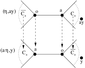
Figure 1. Shift from $(\eta,ay)$ to $(a\eta,y)$ with $x\in C_{a}$

Let $\eta^{\prime}:=a\eta$. Then $(\mathbf{0},a)(\eta,x)=(\eta^{\prime},y)$. Furthermore, $\eta^{\prime}_{a}=a\overline{\eta_{a}}$ and $\overline{\eta^{\prime}_{a}}=a\eta_{a}$. Hence,

$$\ell\bigl{(}(\eta^{\prime},y)\bigr{)}=\ell\bigl{(}(\eta^{\prime}_{a},o)\bigr{)}+\ell\bigl{(}(\overline{\eta^{\prime}_{a}},y)\bigr{)}=\ell\bigl{(}(\eta^{\prime}_{a},o)\bigr{)}+\ell\bigl{(}(a\eta_{a},y)\bigr{)}.$$

As $\overline{\eta_{a}}(w)=1$ if and only if $\eta^{\prime}_{a}(aw)=1$, it follows that

$$\ell\bigl{(}(\eta^{\prime}_{a},o)\bigr{)}=\begin{cases}2+\ell\bigl{(}(\overline{\eta_{a}},o)\bigr{)},&\textrm{if }\overline{\eta_{a}}\not\equiv\mathbf{0}\\ 0,&\textrm{if }\overline{\eta_{a}}\equiv\mathbf{0}\end{cases}.$$

This finishes the proof. ∎

Proposition 3.2.

Let $a\in\mathcal{S}$, $x\in\overline{C_{a}}$ and $\eta\in\mathcal{N}$. Then

$$\ell\bigl{(}(\mathbf{0},a)(\eta,x)\bigr{)}-\ell\bigl{(}(\eta,x)\bigr{)}=\begin{cases}-1,&\textrm{if }\eta_{a}\not\equiv\mathbf{0}\\ 1,&\textrm{if }\eta_{a}\equiv\mathbf{0}\end{cases}.$$

Proof.

Observe again that $\eta_{a}(w)=1$, $\overline{\eta_{a}}(w)=1$ respectively, if and only if $(a\eta_{a})(aw)=1$, $(a\overline{\eta_{a}})(aw)=1$ respectively, for any $w\in\mathcal{T}_{q}$. We obtain

$$\ell\bigl{(}(\eta,x)\bigr{)}=\ell\bigl{(}(\eta_{a},o)\bigr{)}+\ell\bigl{(}(\overline{\eta_{a}},x)\bigr{)}.$$

Furthermore,

$$\ell\bigl{(}(\eta_{a},o)\bigr{)}=\begin{cases}2+\ell\bigl{(}(a\eta_{a},o)\bigr{)},&\textrm{if }\eta_{a}\not\equiv\mathbf{0}\\ 0,&\textrm{if }\eta_{a}\equiv\mathbf{0}\end{cases}.$$

Let $\eta^{\prime}:=a\eta$. Then $(\mathbf{0},a)(\eta,x)=(\eta^{\prime},ax)$. Furthermore, $\eta^{\prime}_{a}=a\overline{\eta_{a}}$ and $\overline{\eta^{\prime}_{a}}=a\eta_{a}$. See Figure 2.

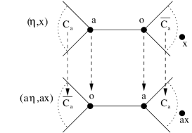
Figure 2. Shift from $(\eta,x)$ to $(a\eta,ax)$ with $x\in\overline{C_{a}}$

Hence,

$$\ell\bigl{(}(\eta^{\prime},ax)\bigr{)}=\ell\bigl{(}(\overline{\eta^{\prime}_{a}},o)\bigr{)}+\ell\bigl{(}(\eta^{\prime}_{a},ax)\bigr{)}=\ell\bigl{(}(a\eta_{a},o)\bigr{)}+1+\ell\bigl{(}(\overline{\eta_{a}},x)\bigr{)}.$$

This finishes the proof. ∎

Proposition 3.3.

Let $(\eta,x)\in\mathcal{N}\times\mathcal{T}_{q}$. Then

$$\ell\bigl{(}(\mathds{1}_{o},o)(\eta,x)\bigr{)}-\ell\bigl{(}(\eta,x)\bigr{)}=\begin{cases}1,&\textrm{if }\eta(o)=0\\ -1,&\textrm{if }\eta(o)=1\end{cases}.$$

Proof.

Obviously, $(\mathds{1}_{o},o)(\eta,x)$ and $(\eta,x)$ differ only by the lamp state at the root $o$, as $(\mathds{1}_{o}\oplus\eta)(o)=1-\eta(o)$. This proves the claim. ∎

Propositions 3.1, 3.2 and 3.3 show that $Y_{g,n}\in\{-1,1\}$. More precisely, $Y_{g,n}$ remains unchanged after the last visit in $o$, that is, $Y_{g,n}$ converges almost surely. By Lebesgue’s Dominated Convergence Theorem, almost sure convergence of the sequence $(\mathbb{E}[\ell(Z_{n+1})-\mathbb{E}[\ell(Z_{n})])_{n\in\mathbb{N}}$ follows. Now we want to compute the integrals $\int Y_{g,n}\,d\mathbb{P}$. For this purpose, we need the following probabilities:

Lemma 3.4.

$$\mathbb{P}[\eta_{\infty}(o)=0]=\frac{q-2+p}{pq+q-2}\quad\textrm{ and }\quad\mathbb{P}[\eta_{\infty}(o)=1]=\frac{p(q-1)}{pq+q-2}.$$

Proof.

Let

$$\widetilde{U} := \mathbb{P}[T_{o}<\infty,X_{1}\neq o]=\sum_{a\in\mathcal{S}}\mu\bigl{(}(\mathbf{0},a)\bigr{)}F=\frac{1-p}{q-1},$$

$$\widetilde{G} := \sum_{n\geq 0}\mathbb{P}\bigl{[}X_{n}=o,\forall j<n:\neg\bigl{(}X_{j}=o\land\mathbf{i}_{j+1}=(\mathds{1}_{o},o)\bigr{)}\bigr{]}$$

$$= \frac{1}{1-\widetilde{U}}=\frac{q-1}{q-2+p}.$$

Now we can compute the proposed probabilities:

$$\mathbb{P}[\eta_{\infty}(o)=0] = \sum_{m\geq 0}\bigl{(}\widetilde{G}\cdot p\bigr{)}^{2m}\cdot\widetilde{G}\cdot(1-p)\cdot(1-F)$$

$$= \frac{q-2+p}{pq+q-2},$$

$$\mathbb{P}[\eta_{\infty}(o)=1] = 1-\mathbb{P}[\eta_{\infty}(o)=0]=\frac{p(q-1)}{pq+q-2}.$$

∎

By Propositions 3.1, 3.2, 3.3 and Lemma 3.4 we obtain

$$\int Y_{g,n}\,d\mathbb{P}=\begin{cases}\frac{(1-p)(q-2)}{pq+q-2},&\textrm{ if }g=(\mathds{1}_{o},o)\\ 1-2\nu_{1}-2\nu_{2},&\textrm{ if }g=(\mathbf{0},a_{i})\textrm{ for some }a_{i}\in\mathcal{S}\end{cases}.$$

Now we can give two explicit formulae for the rate of escape:

Theorem 3.5.

$$\ell = \frac{(1-p)(q-2)}{q}\cdot\Bigl{(}1+2q\nu_{1}+\frac{pq}{pq+q-2}\Bigr{)}$$

$$= \frac{(1-p)(q-2)}{q}\cdot\Bigl{(}\frac{q+1}{q-1}-\frac{2q}{q-1}\nu_{2}+\frac{pq}{pq+q-2}\Bigr{)}$$

Proof.

By Lebesgue’s Dominated Convergence Theorem and the above computations, we get

$$\ell = \sum_{g\in\mathcal{S}_{\mathcal{L}_{q}}}\mu(g)\int\lim_{n\to\infty}\bigl{(}\ell(gZ_{n})-\ell(Z_{n})\bigr{)}\,d\mathbb{P}$$

$$= \sum_{a\in\mathcal{S}}\Bigl{(}\mu\bigl{(}(\mathbf{0},a)\bigr{)}\cdot\bigl{(}1-2\nu_{1}-2\nu_{2}\bigr{)}\Bigr{)}+\mu\bigl{(}(\mathds{1}_{o},o)\bigr{)}\cdot\frac{(1-p)(q-2)}{pq+q-2}$$

$$= (1-p)\cdot(1-2\nu_{1}-2\nu_{2})+\frac{p(1-p)(q-2)}{pq+q-2}.$$

The rest follows by substituting $\nu_{1}=\frac{1}{q-1}(\frac{1}{q}-\nu_{2})$ resp. $\nu_{2}=\frac{1}{q}-(q-1)\nu_{1}$. ∎

Remark: Observe that $\nu_{2}=\check{G}\,\frac{(1-p)}{q}\,(1-F)$ holds, where

$$\check{G}=\sum_{\eta\in\mathcal{N}^{\prime}}G(\eta)\quad\textrm{ with}\quad G(\eta)=\sum_{n\geq 0}p^{(n)}\bigl{(}(\mathbf{0},o),(\eta,o)\bigr{)}$$

and $\mathcal{N}^{\prime}:=\{\eta\in\mathcal{N}\mid\forall w\in\overline{C_{a_{1}}}:\eta(w)=0\}$. The functions $G(\eta)$ are Green functions evaluated at $1$. As Green functions are in general hard to compute or even often not computable and since the structure of the Cayley graph of $\mathcal{L}_{q}$ is very complex, we are only able to give a lower and upper bound for $\ell$ by estimating $\nu_{1}$ and $\nu_{2}$ from below. For this purpose, we need the following lemma:

Lemma 3.6.

Let $z=(\eta_{x},x)\in\mathcal{L}_{q}$ and $y\in\mathcal{T}_{q}$ be a neighbour of $x$ in the tree. Then the probability that the lamplighter, starting at $x$ with configuration $\eta_{x}$, reaches $y$ without changing any lamps is

$$\bar{F}:=\mathbb{P}_{z}\bigl{[}T_{y}<\infty,\forall k<T_{y}:\mathbf{i}_{k}\neq(\mathds{1}_{o},o)\bigr{]}=\frac{q-\sqrt{q^{2}-4(q-1)(1-p)^{2}}}{2(q-1)(1-p)}.$$

Proof.

By vertex-transitivity, we get the recursive equation

$$\bar{F}=\mu\bigl{(}(\mathbf{0},a_{i})\bigr{)}+\sum_{a_{j}\in\mathcal{S}\setminus\{a_{i}\}}\mu\bigl{(}(\mathbf{0},a_{j})\bigr{)}\bar{F}^{2}\quad\textrm{ for any }a_{i}\in\mathcal{S}$$

with solutions

$$\bar{F}=\frac{q\pm\sqrt{q^{2}-4(q-1)(1-p)^{2}}}{2(q-1)(1-p)},$$

where the right one has to to fulfill $\bar{F}<1$. This proves the lemma. ∎

Now we can estimate $\nu_{1}$ and $\nu_{2}$ from below:

Lemma 3.7.

$$\nu_{1} \geq \frac{p}{q(pq+q-2)}=:\widehat{\nu}_{1}\quad\textrm{ and}$$

$$\nu_{2} \geq \frac{\widehat{G}}{1-\widehat{G}^{2}p^{2}}\frac{(1-p)(q-2)}{q(q-1)}=:\widehat{\nu}_{2},$$

where

$$\widehat{G}=\frac{2(q-1)}{q-2+\sqrt{q^{2}-4(q-1)(1-p)^{2}}}.$$

Proof.

We restrict the event $[\eta_{\infty}(C_{a_{1}})\not\equiv\mathbf{0}]$ to the event $[\eta_{\infty}(a_{1})=1]$. Thus,

$$\nu_{1} \geq F\cdot\sum_{m\geq 0}\bigl{(}\widetilde{G}\cdot p\bigr{)}^{2m+1}\cdot\widetilde{G}\cdot\frac{1-p}{q}\cdot\bigl{(}1-F\bigr{)}$$

$$= \frac{p}{q(pq+q-2)}.$$

For the computation of the lower bound of $\nu_{2}$, we introduce some further notation:

$$\widehat{U} := \mathbb{P}\bigl{[}T_{o}<\infty,\forall j<T_{o}:\neg\bigl{(}X_{j}\in\overline{C_{a_{1}}}\land\mathbf{i}_{j+1}=(\mathds{1}_{o},o)\bigr{)}\bigr{]}$$

$$= \frac{q-1}{q}(1-p)\cdot\bar{F}+\frac{1-p}{q}\cdot F,$$

$$\widehat{G} := \sum_{n\geq 0}\mathbb{P}\bigl{[}X_{n}=o,\forall j<n:\neg\bigl{(}X_{j}\in\overline{C_{a_{1}}}\land\mathbf{i}_{j+1}=(\mathds{1}_{o},o)\bigr{)}\bigr{]}$$

$$= \frac{1}{1-\widehat{U}}.$$

We restrict the event $[\eta_{\infty}(\overline{C_{a_{1}}})\equiv\mathbf{0}]$ to the event that no lamps in $\overline{C_{a_{1}}}\setminus\{o\}$ are switched on, that is, $\eta_{n}(\overline{C_{a_{1}}}\setminus\{o\})\equiv\mathbf{0}$ for all $n\in\mathbb{N}$, while we allow to switch the lamp at $o$ for an even number of switches. This yields

$$\nu_{2} \geq \sum_{m\geq 0}\bigl{(}\widehat{G}\cdot p\bigr{)}^{2m}\cdot\widehat{G}\cdot\frac{1-p}{q}\cdot(1-F)$$

$$= \frac{\widehat{G}}{1-\widehat{G}^{2}p^{2}}\cdot\frac{(1-p)(q-2)}{q(q-1)}.$$

∎

Now we can give an upper and lower bound for the rate of escape:

Corollary 3.8.

$$\ell \geq \frac{(1-p)(q-2)}{q}\cdot\frac{q-2+2p(q+1)}{pq+q-2}=:\ell_{\mathrm{low}}\quad\textrm{ and}$$

$$\ell \leq \frac{(1-p)(q-2)}{q}\cdot\Bigl{(}\frac{q+1}{q-1}-\frac{2q}{q-1}\hat{\nu}_{2}+\frac{pq}{pq+q-2}\Bigr{)}=:\ell_{\mathrm{up}}$$

$\square$

Observe that the lower bound also provides $\ell>\lim_{n\to\infty}|X_{n}|/n$ due to the inequality $(q-2+2p(q+1))/(pq+q-2)>1$, that is, the random walk on $\mathcal{L}_{q}$ flees to infinity faster than the projection of the random walk onto $\mathcal{T}_{q}$.

Numerical sample computations are presented at the end of the next section.

4. Another Lower Bound

We construct another lower bound for $\ell$, which is better than $\ell_{\mathrm{low}}$ if $p\leq\frac{q-2}{q-1}$. For this purpose, we give another lower bound for $\nu_{1}$, and then apply Theorem 3.5.

Observe that

$$\nu_{1}=F\cdot\underbrace{\mathbb{P}[a\textrm{ is first letter of }X_{\infty},\eta_{\infty}(\overline{C_{a_{1}}})\not\equiv\mathbf{0}]}_{=:\nu_{3}}.$$

Observe that $\eta_{\infty}(\overline{C_{a_{1}}})\not\equiv\mathbf{0}$ means that at least one lamp in $\overline{C_{a_{1}}}$ rests on forever. Now we distinguish which of the lamps in $\overline{C_{a_{1}}}\cap\mathrm{supp}\,\eta_{\infty}$ is the first lamp to be switched on and rests finally on, while it is allowed to turn it off temporarily. More formally, define the random variable $\mathbf{l}_{1}$ such that $\mathbf{l}_{1}=x\in\overline{C_{a_{1}}}$ if $X_{n}=X_{n+1}=x$ holds for some $n\in\mathbb{N}$ with $\eta_{m}(y)=0$ for all $m<n$ and all $y\in\overline{C_{a_{1}}}\cap\mathrm{supp}\,\eta_{\infty}$. It is sufficient to define $\mathbf{l}_{1}$ only on the event $\bigl{[}\eta_{\infty}(\overline{C_{a_{1}}})\not\equiv\mathbf{0}\bigr{]}$. Define

$$L := \sum_{n\geq 1}\mathbb{P}[X_{n}=a_{1},\forall m\in\{1,\dots,n\}:X_{m}\neq o]$$

$$= \frac{1-p}{q}\cdot\sum_{n\geq 0}\Bigl{(}\frac{q-1}{q}(1-p)F+p\Bigr{)}^{n}=\frac{1}{q-1}$$

and

$$\bar{G}:=\sum_{n\geq 0}\mathbb{P}\bigl{[}X_{n}=o,\forall k\leq n:\mathbf{i}_{k}\neq(\mathds{1}_{o},o)\bigr{]}=\frac{1}{1-(1-p)\bar{F}}.$$

Now

$$\nu_{3} = \sum_{x\in\overline{C_{a_{1}}}}\mathbb{P}[a_{1}\textrm{ is first letter of }X_{\infty},\eta_{\infty}(\overline{C_{a_{1}}})\not\equiv\mathbf{0},\mathbf{l}_{1}=x]$$

$$\geq \sum_{x\in\overline{C_{a_{1}}}}\bar{F}^{|x|}\cdot\bar{G}\cdot\sum_{m\geq 0}\bigl{(}p\,\widetilde{G}\bigr{)}^{2m+1}\cdot L^{|x|}\cdot\frac{1-p}{q}\cdot(1-F)$$

$$= \frac{\bar{G}\widetilde{G}p}{1-p^{2}\widetilde{G}^{2}}\cdot\frac{1-p}{q}\cdot\frac{q-2}{q-1}\cdot\sum_{n\geq 0}(q-1)^{n}\bigl{(}\bar{F}\cdot L\bigr{)}^{n}$$

$$= \frac{\bar{G}\widetilde{G}p}{1-p^{2}\widetilde{G}^{2}}\cdot\frac{1-p}{q}\cdot\frac{q-2}{q-1}\cdot\frac{1}{1-\bar{F}}$$

$$= \frac{p(q-2+p)}{q(pq+q-2)(1-\bar{F})(1-(1-p)\bar{F})}=:\widehat{\nu}_{3}.$$

Thus,

$$\ell\geq\frac{(1-p)(q-2)}{q}\cdot\Bigl{(}1+2\frac{q}{q-1}\widehat{\nu}_{3}+\frac{pq}{pq+q-2}\Bigr{)}=\ell_{\mathrm{low},2}.$$

With the help of mathematica we can show that $\ell_{\mathrm{low},2}\geq\ell_{\mathrm{low}}$ if $p\leq\frac{q-2}{q-1}$.

Table 3 compares the values of the trivial lower bound given by $\lim_{n\to\infty}|X_{n}|/n=(1-p)(q-2)/q$, the lower bounds $\ell_{\mathrm{low}}$ and $\ell_{\mathrm{low},2}$ and the upper bound $\ell_{\mathrm{up}}$ for different values of $q$ and $p$. The relative precision of the approximation is the quotient

$$\frac{\ell_{\mathrm{up}}-\max\{\ell_{\mathrm{low}},\ell_{\mathrm{low},2}\}}{1-\lim_{n\to\infty}\frac{|X_{n}|}{n}},$$

which decreases when the degree $q$ of the tree increases: large $q$ yields tighter bounds.

$q$	$p$	$\lim_{n\to\infty}\frac{|X_{n}|}{n}$	$\ell_{\mathrm{low}}$	$\ell_{\mathrm{low},2}$	$\ell_{\mathrm{up}}$	$\begin{subarray}{c}\mathrm{relative}\\ \mathrm{precision}\end{subarray}$
3	4/5	0.067	0.145098	0.144410	0.157358	0.01314
3	2/3	0.111	0.234567	0.233467	0.253778	0.02161
3	1/2	0.167	0.333	0.333	0.359733	0.03167
3	1/4	0.25	0.428571	0.438050	0.461289	0.03099
5	4/5	0.12	0.216	0.215942	0.221533	0.00629
5	2/3	0.2	0.347368	0.347629	0.355735	0.010459
5	1/2	0.3	0.490909	0.492585	0.501825	0.01559
5	1/4	0.45	0.635294	0.641344	0.647154	0.01056
10	4/5	0.16	0.256	0.256029	0.257516	0.001805
10	2/3	0.267	0.412121	0.412311	0.414351	0.003040
10	1/2	0.4	0.584615	0.585277	0.587408	0.00465
10	1/4	0.6	0.771429	0.773099	0.774202	0.00276
20	4/5	0.18	0.273176	0.273189	0.273569	0.0004789
20	2/3	0.3	0.440425	0.440487	0.440994	0.0008128
20	1/2	0.45	0.626785	0.626975	0.627483	0.001269
20	1/4	0.675	0.836413	0.836835	0.837079	0.00075

Figure 3. Sample computations of lower and upper bounds

5. Further Random Walk Models

We now consider two other models of lamplighter random walks on $\mathcal{T}_{q}$ and give lower bounds for the acceleration as compared with their projection onto the tree.

5.1. Switch-Walk-Switch

Consider again the wreath product $(\mathbb{Z}/2)\wr\mathcal{T}_{q}$, but now with generating set

$$\mathcal{S}_{\mathcal{L}_{q}}^{\ast}:=\bigl{\{}(\mathds{1}_{A},a)\mid a\in\mathcal{S},A\in\{\emptyset,\{o\},\{a\},\{o,a\}\}\bigr{\}}.$$

Consider the random walk on the Cayley graph of $(\mathbb{Z}/2)\wr\mathcal{T}_{q}$ wrt. $\mathcal{S}_{\mathcal{L}_{q}}^{\ast}$ described by the sequence of random variables $\bigl{(}Z_{n}\bigr{)}_{n\in\mathbb{N}_{0}}$ valued in $(\mathbb{Z}/2)\wr\mathcal{T}_{q}$ with $Z_{0}=(\mathbf{0},o)$, which is governed by the probability measure $\mu^{\ast}$ on $\mathcal{S}_{\mathcal{L}_{q}}$ instead of $\mu$, where

$$\mu^{\ast}\bigl{(}(\mathds{1}_{A},a_{i})\bigr{)}=\begin{cases}\frac{(1-p)^{2}}{q}&\textrm{, if }A=\emptyset\\ \frac{p(1-p)}{q}&\textrm{, if }|A|=1\\ \frac{p^{2}}{q}&\textrm{, if }|A|=2\\ \end{cases}.$$

This random walk can be interpreted as follows: In one step the lamplighter may flip the lamp state at his actual position with probability $p$, walks along one adjacent random edge with probability $1/q$ and may flip the lamp state at the destination vertex with probability $p$. The number $\ell(Z_{n})$ is then the graph distance of $Z_{n}$ to $(\mathbf{0},o)$ in the Cayley graph of $(\mathbb{Z}/2)\wr\mathcal{T}_{q}$ wrt. $\mathcal{S}^{\ast}_{\mathcal{L}_{q}}$. Write again $Z_{n}=(\eta_{n},X_{n})$. Thus, $(X_{n})_{n\in\mathbb{N}_{0}}$ is simple random walk on $\mathcal{T}_{q}$.

It is well-known that $\lim_{n\to\infty}|X_{n}|/n=(q-2)/q$. Our aim is to estimate the ratio of $\ell=\lim_{n\to\infty}\ell(Z_{n})/n$ and $(q-2)/q$. Define for $k\in\mathbb{N}_{0}$ the exit times

$$\mathbf{e}_{k} := \min\bigl{\{}m\in\mathbb{N}_{0}\ \bigl{|}\ |X_{m}|=k\land\forall n\geq m:X_{n}\in C_{X_{m}}\bigr{\}}.$$

By transience we have almost surely $\mathbf{e}_{k}<\infty$ for all $k\in\mathbb{N}_{0}$. Define now for $k\in\mathbb{N}$ the pseudo-increments

$$\Delta_{k}:=\begin{cases}0,&\textrm{ if }\eta_{\mathbf{e}_{k}}(w)=0\textrm{ for all }w\in C_{X_{\mathbf{e}_{k-1}}}\setminus(C_{X_{\mathbf{e}_{k}}}\cup\{X_{\mathbf{e}_{k-1}}\})\\ 2,&\textrm{ otherwise}\end{cases}.$$

The set $C_{X_{\mathbf{e}_{k-1}}}\setminus(C_{X_{\mathbf{e}_{k}}}\cup\{X_{\mathbf{e}_{k-1}}\})$ is the union of the cones $C_{z}$, where $z$ is a forward neighbour of $X_{\mathbf{e}_{k-1}}$ distinct from $X_{\mathbf{e}_{k}}$. The pseudo-increment $\Delta_{k}$ represents a lower bound for the length of a possible deviation inside $C_{X_{\mathbf{e}_{k-1}}}\setminus C_{X_{\mathbf{e}_{k}}}$, when walking from $o$ to $X_{n}$, where $\mathbf{e}_{k}<n$, with restoring the configuration $\eta_{n}$. Note that a shortest tour from $o$ to $X_{n}$ does not visit $C_{X_{\mathbf{e}_{k-1}}}\setminus(C_{X_{\mathbf{e}_{k}}}\cup\{X_{\mathbf{e}_{k-1}}\})$. If at time $\mathbf{e}_{k-1}$ the lamplighter stands at $g=g^{\prime}a_{1}\in\mathcal{T}_{q}$, then walks to $ga_{i}$, $i\notin\{1,q\}$, thereby switching the lamp at $ga_{i}$ on, walks back to $g$ without flipping the lamp state at $ga_{i}$, followed by walking to $ga_{q}$ and rests henceforth in $C_{ga_{q}}$, then $\Delta_{k}=2$. See Figure 4.

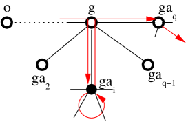
Figure 4. Interpretation of $\Delta_{k}$

Observe that we have for all $k\geq 1$

$$(*)\quad\quad\ell\bigl{(}(\eta_{\mathbf{e}_{k}},Z_{\mathbf{e}_{k}})\bigr{)}\geq k+\sum_{j=1}^{k}\Delta_{j}.$$

To estimate the distribution of $\Delta_{k}$, we distinguish if at time $\mathbf{e}_{k-1}$ lamps are on in $C_{X_{\mathbf{e}_{k-1}}}\setminus\{X_{\mathbf{e}_{k}-1}\}$ or not and if lamps are on in $C_{X_{\mathbf{e}_{k-1}}}\setminus\bigl{(}C_{X_{\mathbf{e}_{k}}}\cup\{X_{\mathbf{e}_{k-1}}\}\bigr{)}$ at time $\mathbf{e}_{k}$. For $x\in\mathcal{T}_{q}\setminus\{o\}$ we use the notation $x^{-}$ to express the unique neighbour of $x$ closer to $o$. For $k\in\mathbb{N}$ let

$$E := \bigl{\{}(\eta,x)\in\mathcal{N}\times(\mathcal{T}_{q}\setminus\{o\})\ \bigl{|}\ \exists w\in C_{x^{-}}\setminus(C_{x}\cup\{x^{-}\}):\eta(w)=1\bigr{\}},$$

$$E_{k,0} := \bigl{\{}(\eta,x)\in\mathcal{N}\times\mathcal{T}_{q}\ \bigl{|}\ |x|=k,\forall w\in C_{x}\setminus\{x\}:\eta(w)=0\bigr{\}}\quad\textrm{ and}$$

$$E_{k,2} := \bigl{\{}(\eta,x)\in\mathcal{N}\times\mathcal{T}_{q}\ \bigl{|}\ |x|=k,\exists w\in C_{x}\setminus\{x\}:\eta(w)=1\bigr{\}}.$$

Observe that for $k\geq 2$ and $r\in\{0,2\}$ it is

$$\mathbb{P}[Z_{\mathbf{e}_{k-1}}\in E_{k-1,r}]=\sum_{m\geq 0}\sum_{(\eta,x)\in E_{k-1,r}}\mathbb{P}\bigl{[}X_{m-1}=x^{-},Z_{m}=(\eta,x)\bigr{]}\cdot\bigl{(}1-F\bigr{)}.$$

Thus,

$$\mathbb{P}[\Delta_{k}=2\mid Z_{\mathbf{e}_{k-1}}\in E_{k-1,r}]$$

$$= \frac{1}{\mathbb{P}[Z_{\mathbf{e}_{k-1}}\in E_{k-1,r}]}\sum_{m\geq 0}\sum_{(\eta,x)\in E_{k-1,r}}\mathbb{P}\bigl{[}X_{m-1}=x^{-},Z_{m}=(\eta,x)\bigr{]}\cdot$$

$$\quad\cdot\Bigl{(}\sum_{l\geq 1}\mathbb{P}_{(\eta,x)}\bigl{[}\forall\tau\leq l:X_{\tau}\neq x^{-},X_{l-1}=x,(\eta_{l},X_{l})\in E\bigr{]}\Bigl{)}\cdot\bigl{(}1-F\bigr{)}$$

$$\geq \inf_{(\eta,x)\in E_{k-1,r}}\sum_{l\geq 1}\mathbb{P}_{(\eta,x)}\bigl{[}\forall\tau\leq l:X_{\tau}\neq x^{-},X_{l-1}=x,(\eta_{l},X_{l})\in E\bigr{]}.$$

Now we can prove:

Lemma 5.1.

We have $\mathbb{E}[\Delta_{k}]\geq B$ for all $k\in\mathbb{N}$, where

$$B:=\frac{4}{q^{3}}\cdot(q-1)\cdot(q-2)\cdot p\cdot(1-p)>0.$$

Proof.

Let $k\in\mathbb{N}$. By the above computations we get

$$\mathbb{P}[\Delta_{k}=2\mid Z_{\mathbf{e}_{k-1}}\in E_{k-1,0}]\geq 2\cdot(q-1)\cdot\frac{p(1-p)}{q^{2}}\cdot\frac{q-2}{q}=\frac{1}{2}B>0$$

and

$$\mathbb{P}[\Delta_{k}=2\mid Z_{\mathbf{e}_{k-1}}\in E_{k-1,2}]\geq\frac{q-2}{q}\geq\frac{1}{2}B.$$

Thus, we obtain for $k\geq 2$

$$\mathbb{E}[\Delta_{k}] = \mathbb{P}[Z_{\mathbf{e}_{k-1}}\in E_{k-1,0}]\cdot\mathbb{E}[\Delta_{k}\mid Z_{\mathbf{e}_{k-1}}\in E_{k-1,0}]$$

$$\quad+\mathbb{P}[Z_{\mathbf{e}_{k-1}}\in E_{k-1,2}]\cdot\mathbb{E}[\Delta_{k}\mid Z_{\mathbf{e}_{k-1}}\in E_{k-1,2}]\geq B>0.$$

We have to handle the case $k=1$ separately: here, we have $\mathbb{P}[Z_{\mathbf{e}_{0}}\in E_{0,0}]=1$ and thus

$$\mathbb{E}[\Delta_{1}]\geq 4\cdot q\cdot\frac{p(1-p)}{q^{2}}\cdot\frac{q-1}{q}\geq B.$$

∎

Now we want to prove the acceleration on the lamplighter tree:

Theorem 5.2.

For the switch-walk-switch lamplighter random walk,

$$\ell\geq\frac{q-2}{q}\cdot(1+B).$$

Proof.

Observe that

$$\frac{q-2}{q}=\lim_{k\to\infty}\frac{|X_{\mathbf{e}_{k}}|}{\mathbf{e}_{k}}=\lim_{k\to\infty}\frac{|X_{\mathbf{e}_{k}}|}{k}\frac{k}{\mathbf{e}_{k}}=\lim_{k\to\infty}\frac{k}{\mathbf{e}_{k}}.$$

Furthermore,

$$\ell=\lim_{k\to\infty}\frac{\ell(Z_{\mathbf{e}_{k}})}{\mathbf{e}_{k}}=\lim_{k\to\infty}\frac{\ell(Z_{\mathbf{e}_{k}})}{k}\frac{k}{\mathbf{e}_{k}}=\frac{q-2}{q}\lim_{k\to\infty}\frac{\ell(Z_{\mathbf{e}_{k}})}{k}\quad\mathbb{P}-a.s..$$

As $\ell>0$, the limit $\ell_{0}=\lim_{k\to\infty}\ell(Z_{\mathbf{e}_{k}})/k$ exists almost surely and is almost surely constant. We show now that this limit is greater than $1$. By equation $(*)$

$$\frac{\ell(Z_{\mathbf{e}_{k}})}{k}\geq 1+\frac{1}{k}\sum_{j=1}^{k}\Delta_{j}.$$

Define $D_{k}:=\frac{1}{k}\sum_{j=1}^{k}\Delta_{j}$. Then $0\leq D_{k}\leq 2$ and by Lemma 5.1

$$\mathbb{E}[D_{k}]\geq B>0.$$

As $\limsup_{k\in\mathbb{N}}D_{k}=2-\liminf_{k\in\mathbb{N}}(2-D_{k})$, we can apply Fatou’s Lemma and obtain

$$\mathbb{E}[\limsup_{k\in\mathbb{N}}D_{k}] = 2-\int\liminf_{k\in\mathbb{N}}(2-D_{k})\,d\mathbb{P}$$

$$\geq 2-\liminf_{k\in\mathbb{N}}\int(2-D_{k})\,d\mathbb{P}=\limsup_{k\in\mathbb{N}}\mathbb{E}[D_{k}].$$

As $\ell_{0}\geq 1+\limsup_{k\in\mathbb{N}}D_{k}$ we can conclude:

$$\ell_{0}\geq 1+\mathbb{E}[\limsup_{k\in\mathbb{N}}D_{k}]\geq 1+\limsup_{k\in\mathbb{N}}\mathbb{E}[D_{k}]\geq 1+B.$$

This finishes the proof. ∎

It is also possible to construct lower and upper bounds for the rate of escape of this random walk by the technique used in the previous section. Numerical computations show that those bounds are less tight than in the case of Section 3, that is, the spread between the bounds is greater.

5.2. Several Lamp States

Assume now that there sits a lamp at each vertex of $\mathcal{T}_{q}$, which can take $r$ different lamp states including off. These different lamp states are encoded by elements of $\mathbb{Z}/r$, where $0$ represents the state “off”. Consider now the wreath product $(\mathbb{Z}/r)\wr\mathcal{T}_{q}$ with generating set

$$\mathcal{S}^{(r)}_{\mathcal{L}_{q}}:=\bigl{\{}(k\mathds{1}_{o},o),(\mathbf{0},a_{i})\mid k\in\{1,\dots,r-1\},a_{i}\in\mathcal{S}\bigr{\}}.$$

Given $p\in(0,1)$. Choose $\alpha_{1},\dots,\alpha_{r-1}$ such that $\sum_{k=1}^{r-1}\alpha_{k}=p$. Then the corresponding random walk on the lamplighter tree, where each lamp can take $r$ different lamp states, is the random walk on the Cayley graph of $(\mathbb{Z}/r)\wr\mathcal{T}_{q}$, which is governed by the probability measure $\mu_{r}$ on $\mathcal{S}^{(r)}_{\mathcal{L}_{q}}$:

$$\mu_{r}(z):=\begin{cases}\alpha_{k}&\textrm{, if }z=(k\mathds{1}_{o},o)\\ \frac{1-p}{q}&\textrm{, otherwise}\end{cases}.$$

For any $z\in(\mathbb{Z}/r)\wr\mathcal{T}_{q}$ it is $\ell(z)=\min\{n\mid\mu_{r}^{(n)}(z)>0\}$, where $\mu_{r}^{(n)}$ is the $n$-th convolution power of $\mu_{r}$. Analogous to Section 5.1 we can show that the corresponding rate of escape $\lim_{n\to\infty}\ell(Z_{n})/n$ is strictly greater than the drift of its projection onto $\mathcal{T}_{q}$, namely $\lim_{n\to\infty}|X_{n}|/n=(1-p)(q-2)/q$, where $X_{n}\in\mathcal{T}_{q}$ is the random position of the lamplighter at time $n$.

References

- [1] D. Bertacchi. Random walks on Diestel-Leader graphs. Abh. Math. Sem. Univ. Hamburg, 71:205–224, 2001.
- [2] D. Cartwright, V. Kaimanovich, and W. Woess. Random walks on the affine group of local fields and of homogenous trees. Ann. Inst. Fourier (Grenoble), 44:1243–1288, 1994.
- [3] Y. Derriennic. Quelques applications du théorème ergodique sous-additif. Astérisque, 74:183–201, 1980.
- [4] A. Dyubina. Characteristics of random walks on wreath products of groups. J. of Math. Sciences, 107(5):4166–4171, 2001.
- [5] A. Erschler. On the asymptotics of drift. J. of Math. Sciences, 121(3):2437–2440, 2004.
- [6] H. Furstenberg. Non commuting random products. Trans. Amer. Math. Soc., 108:377–428, 1963.
- [7] L. A. Gilch. Rate of escape of random walks on free products. Journal of Australian Mathematical Society, to appear.
- [8] Y. Guivarc’h. Sur la loi des grands nombres et le rayon spectral d’une marche aléatoire. Astérisque, 74:47–98, 1980.
- [9] V. Kaimanovich and A. Vershik. Random walks on discrete groups: boundary and entropy. Ann. Probab., 11:457–490, 1983.
- [10] J. Kingman. The ergodic theory of subadditive processes. J. Royal Stat. Soc., Ser. B, 30:499–510, 1968.
- [11] F. Ledrappier. Some asymptotic properties of random walks on free groups. In CRM Proceedings and Lecture Notes, volume 28, pages 117–152. CRM, 2001.
- [12] R. Lyons, R. Pemantle, and Y. Peres. Random walks on the lamplighter group. Ann. of Probability, 24(4):1993–2006, 1996.
- [13] J. Mairesse. Randomly growing braid on three strands and the manta ray. Report LIAFA 2005-001, Univ. Paris 7, 2005.
- [14] T. Nagnibeda and W. Woess. Random walks on trees with finitely many cone types. J. Theoret. Probab., 15:399–438, 2002.
- [15] D. Revelle. Rate of escape of random walks on wreath products and related groups. The Annals of Probability, 31(4):1917–1934, 2003.
- [16] N. T. Varopoulos. Long range estimates for Markov chains. Bull. Sc. math., 109:225–252, 1985.