The optical emission line spectrum of Mark 110

Abstract

Aims. We analyse in detail the rich emission line spectrum of Mark 110 to determine the physical conditions in the nucleus of this object, a peculiar NLS1 without any detectable Fe II emission associated with the broad line region and with a $\lambda$5007/H$\beta$ line ratio unusually large for a NLS1.

Methods. We use 24 spectra obtained with the Marcario Low Resolution Spectrograph attached at the prime focus of the 9.2 m Hobby-Eberly telescope at the McDonald observatory. We fitted the spectrum by identifying all the emission lines (about 220) detected in the wavelength range 4200-6900 Å (at rest).

Results. The narrow emission lines are probably produced in a region with a density gradient in the range 10³-10⁶ cm^-3 with a rather high column density (5$\times$10²¹ cm^-2). In addition to a narrow line system, three major broad line systems with different line velocity and width are required. We confirm the absence of broad Fe II emission lines. We speculate that Mark 110 is in fact a BLS1 with relatively ”narrow” broad lines but with a BH mass large enough compared to its luminosity to have a lower than Eddington luminosity.

1 Introduction

Narrow line Seyfert 1 galaxies (NLS1s) are Seyfert 1 galaxies in which the broad emission lines are relatively narrow ($<$2 000 km s^-1 FWHM)(Osterbrock & Pogge osterbrock85 (1985)). These objects generally have strong Fe II emission and relatively weak [O III]$\lambda$5007 emission (Boroson & Green boroson92 (1992)). However Grupe et al. (grupe99 (1999); grupe04 (2004)) have found a few objects with ”narrow” broad Balmer lines which have both weak Fe II emission and strong [O III]. Mark 110, Kaz 320 and HS 0328+0528 are three such objects. 1RXS J102012.6+342837 and 1RXS J133209.8+842412 could be two additional exemples (Wu et al. wu03 (2003)).

The aim of this paper is to study the rich optical emission line spectrum of Mark 110, one of these rare objects.

In section 2 we describe the target Mark 110 and present the observations in section 3. In section 4 we analyse the emission line spectrum and in section 5 we determine the physical conditions in the NLR, discuss the various determinations of the BH mass and the true nature of Mark 110: NLS1 or BLS1. Our conclusions are summarized in section 6.

2 The target

Mark 110 (0921+52) was discovered by Markaryan (markaryan69 (1969)) in the course of a slitless spectroscopic survey for UV excess galaxies. It was classified as a Seyfert 1 (Arakelyan et al. arakelyan70 (1970)). The starlike object located 6$\arcsec$ to the north east of the nucleus is a star. The galaxy has a disturbed morphology suggestive of a recent merger (Wehinger & Wyckoff wehinger77 (1977); Adams adams77 (1977); Hutchings & Craven hutchings88 (1988); McKenty mckenty90 (1990); Bischoff & Kollatschny bischoff99 (1999)). The Galactic extinction is A_V=0.056 mag. (Schlegel et al. schlegel98 (1998)). The redshift, measured from the [O III]$\lambda$5007 line is z=0.0352 (Vrtilek & Carleton vrtilek85 (1985)). The H$\beta$ FWHM lies in the range 1 670-2 500 km s^-1 (Osterbrock osterbrock77 (1977); Peterson et al. peterson85 (1985); Crenshaw crenshaw86 (1986); Boroson & Green boroson92 (1992); Bischoff & Kollatschny bischoff99 (1999); Stepanian et al. stepanian03 (2003); Grupe et al. grupe04b (2004)). Bischoff & Kollatschny (bischoff99 (1999)) and Grupe et al. (grupe04b (2004)) classified it as an NLS1 on the basis of its H$\beta$ FWHM (1670$\pm$50 and 1760$\pm$50 km s^-1 respectively) measured after removal of the narrow component.

The optical continuum of Mark 110 is variable (Peterson et al. peterson84 (1984); peterson98 (1998)) with possible intranight variability (Webb & Malkan webb00 (2000)). The broad emission lines show strong variability (Peterson et al. peterson85 (1985); Peterson peterson88 (1988)). The r.m.s. spectrum clearly shows H$\alpha$, H$\beta$ and H$\gamma$, He II $\lambda$4686 and the He I $\lambda$4471, $\lambda$4922, $\lambda$5016, $\lambda$5876 and $\lambda$6678 lines. The [Fe X] $\lambda$6375 line is also variable (Kollatschny et al. kollatschny01 (2001)).

The He II $\lambda$4686 line shows the largest variation of nearly a factor of 8 within two years. On the other hand H$\beta$ and the continuum at 5100 Å vary only by a factor of 1.7 and 3.0 respectively within the same time interval (Bischoff & Kollatschny bischoff99 (1999); Peterson et al. peterson98 (1998); peterson04 (2004)).

There is a very broad component ($\sim$5 000 km s^-1 FWHM), redshifted by 400$\pm$100 km s^-1 with respect to the narrow lines, visible in the Balmer line profiles especially when the continuum is strong. This very broad component is the strongest contributor to the He II variability (Bischoff & Kollatschny bischoff99 (1999)). The outer wings of the line profiles respond much faster to continuum variations than the central regions (Kollatschny 2003a ).

The Fe II emission is weak (the line ratio relative to H$\beta$ is R₄₅₇₀=0.09-0.16) (Osterbrock osterbrock77 (1977); Meyers & Peterson meyers85 (1985); Boroson & Green boroson92 (1992)). The Fe II line flux remains constant while the Balmer line flux varies (Bischoff & Kollatschny bischoff99 (1999)).

3 The observations

Twenty six spectra of Mark 110 have been obtained between 1999, November 13 and 2000, May 14 with the Marcario Low Resolution Spectrograph (LRS) attached at the prime focus of the 9.2-m Hobby-Eberly telescope (HET) at McDonald observatory. The log of the observations is given in Table 1. The detector was a 3072$\times$1024 15 $\mu$m pixel Ford Aerospace CCD with 2$\times$2 binning. The spectra cover the wavelength range 4200-6900 Å in the restframe of the galaxy, with a resolving power of 650 at 5000 Å (7.7 Å FWHM). Exposure times were 10 to 20 min. The slit width was 2$\aas@@fstack{\prime\prime}$0 (i.e. 75 $\mu$m or 3 pixels on the detector). Seven columns were extracted, corresponding to 3$\aas@@fstack{\prime\prime}$3 on the sky. Observations of several spectrophotometric standard stars were obtained to allow flux calibration of the spectra which have not been corrected for atmospheric absorption. Wavelength calibration was achieved via observations of HgCdZn and Ne spectra (Kollatschny et al. kollatschny01 (2001)). Two of the spectra (2000 February 21 and April 30) of lower quality were ignored. All spectra were deredshifted using z=0.0355 .

We give in cols. 3 and 4 of Table 1 the continuum flux in the wavelength range 5130-5140 Å as measured by Kollatschny et al. (kollatschny01 (2001)) and the continuum flux at 5100 Å as obtained from our fit, i.e. the value at 5100 Å of the polynomial used for the continuum in the simultaneous fit of all emission lines in each individual spectrum after subtraction of an elliptical template (see below). In principle the difference between these two sets of numbers should be constant. It is not the case because of the different procedures used.

Table 1: Log of observations. Col. 1: Julian date-2 400 000, col. 2: UT date, col. 3: continuum fluxes at 5100 Å measured by Kollatschny et al. (kollatschny01 (2001)), col. 4: our measurements of the continuum flux (in unit of 10^-15 erg^-1 cm^-2 Å^-1) after removal of the host galaxy contribution.

JD	UT date	col. 3	col. 4
51495.94	1999.11.13	1.54	1.26
51497.91	1999.11.15	1.56	1.25
51500.91	1999.11.18	1.65	1.34
51518.89	1999.12.06	1.92	1.51
51520.87	1999.12.08	1.92	1.53
51522.88	1999.12.10	1.94	1.53
51525.84	1999.12.13	1.82	1.46
51528.84	1999.12.16	1.86	1.49
51547.80	2000.01.04	2.15	1.75
51584.72	2000.02.10	1.41	1.10
51586.71	2000.02.12	1.39	1.08
51598.86	2000.02.24	1.63	1.30
51605.83	2000.03.02	1.40	1.10
51608.62	2000.03.05	1.35	1.07
51611.62	2000.03.08	1.36	1.07
51614.63	2000.03.11	1.09	0.80
51629.76	2000.03.26	1.08	0.80
51637.77	2000.04.03	1.04	0.77
51645.73	2000.04.11	1.16	0.89
51658.70	2000.04.24	1.38	1.12
51663.68	2000.04.29	1.26	0.96
51670.70	2000.05.06	1.33	1.01
51673.69	2000.05.09	1.11	0.85
51678.64	2000.05.14	1.11	0.82

4 Analysis

Using an HST image of Mark 110, Bentz et al. (bentz06 (2006)) have shown that the contribution of the host galaxy in a 5$\aas@@fstack{\prime\prime}$0$\times$7$\aas@@fstack{\prime\prime}$6 aperture is equal to 1.11$\times$10^-15 erg s^-1 cm^-2 Å^-1. We have measured the contribution of this galaxy in the 2$\aas@@fstack{\prime\prime}$0$\times$3$\aas@@fstack{\prime\prime}$3 aperture used here on the HST image (taken through a filter centered at 5580 Å) kindly provided to us by M.C. Bentz to be 55% of this value, i.e. 0.61$\times$10^-15 erg s^-1 cm^-2 Å^-1. By trial and error, we estimated the contribution of the host galaxy, assumed to be an E galaxy, to be 0.25$\times$10^-15 erg s^-1cm^-2 Å^-1 in our entrance aperture at 5100 Å . This is significantly smaller than the value inferred from the HST image. It could be due to the fact that the host galaxy is of a latter type with shallower absorption lines. The assumption that the host is an E galaxy is justified by the fact that Bentz et al. (bentz06 (2006)) have obtained a good fit of the image by using a central PSF and a de Vaucouleurs profile. We have subtracted from all spectra the spectrum of an E galaxy with our estimated flux density.

Figure 1: The mean deredshifted HET spectrum of Mark 110. The upper panel shows the spectrum. In the lower panel it is scaled to show the weak emission features. The residuals of the best fit are also shown.

We have averaged the 24 high quality HET spectra. This mean spectrum is shown in Fig. 1. To identify all individual emission lines and achieve a good fit of this spectrum, in addition to a narrow line system, three major line systems with different line velocity and width are required.

4.1 The narrow line system

Two components were needed to fit the strong narrow lines. The second, fainter, system is redshifted with respect to the first by 220 km s^-1. The H$\beta$ line ratio of these two systems is 0.20.

The intrinsic [O III]$\lambda$5007 FWHM is equal to 280$\pm$3 km s^-1 (Feldman et al. feldman82 (1982)) or 288$\pm$5 km s^-1 (Vrtilek & Carleton vrtilek85 (1985)). The resolution of our spectra is 475 km s^-1; we should therefore measure a FWHM of 550 km s^-1. The measured FWHM of the two components of [O III] $\lambda$5007 are equal to 520 and 470 km s^-1 respectively.

The [O III] $\lambda$5007 flux density has been measured to be equal to (2.26$\pm$0.14)$\times$10^-13 erg s^-1 cm^-2 by Peterson et al. (peterson98 (1998)). The spectra we used in this paper have been calibrated by Bischoff & Kollatschny (bischoff99 (1999)) in such a way that the [O III] $\lambda$5007 flux density is equal to this value. Adding the flux of the two components needed in our model to fit this line, we obtain 2.19 $\times$10^-13 erg s^-1 cm^-2.

The lines observed in the stonger system are listed in Table 5. They include lines of highly ionised ions ([Fe VI], [Fe VII], [Fe X], [Ca V], [Ca VII] which are slightly resolved (640 km s^-1 measured FWHM) and redshifted by $\sim$80 km s^-1 with respect to the Balmer lines. De Robertis & Osterbrock (robertis84 (1984)) and Appenzeller & Ostreicher (appenzeller88 (1988)) have observed high-ionization lines in the emission spectrum of some Seyfert galaxies. In these objects, the very high ionization lines, especially those of [Fe VII], [Fe X] have FWHM which are broader that the typical low-ionization lines such as [O I] or [N I].

The other lines, mostly from permitted and forbidden Fe II and Ti II, are redshifted by 100 km s^-1 with respect to the [O III] lines. The observed permitted Fe II multiplets are listed in Table 2. We have identified a line observed at $\sim$4480 Å with Mg II 4 $\lambda$4481. This line has been observed in emission in the eclipsing dwarf nova IP Peg (Harlaftis harlaftis99 (1999)) and in the ”iron star” XX Oph (Merrill merrill61 (1961); Cool et al. cool05 (2005)).

Table 2: Observed permitted Fe II multiplets in the narrow line system of the spectrum of Mark 110. Col. 1: multiplet number, col. 2: transition, col. 3: upper level energy, col. 4: number of observed lines/number of lines in the multiplet in the observed spectral range.

m.	Transition	u.l.(eV)
42	a6S-z6Po	5.34	3/3
27	b4P-z4Do	5.56	1/6
38	b4F-z4Do	5.56	6/9
43	a6S-z4Do	5.56	1/3
37	b4F-z4Fo	5.57	6/10
49	a4G-z4Fo	5.57	6/9
55	b2H-z4Fo	5.57	1/3

This system shares many similarities with the emission line spectrum of the symbiotic nova RR Tel (McKenna et al. mckenna97 (1997); Crawford et al. crawford99 (1999)) and that of XX Oph. The lines in XX Oph consist primarily of hydrogen and ionized metals such as Fe II, Cr II and Ti II. Collin & Joly (collin00 (2000)) have noted that several types of stars, such as cataclysmic binaries, display intense Fe II lines; it is believed that these lines are formed in the accretion disk. They suggested that physical conditions leading to their formation are similar to those in NLS1s. The fact that lines of Fe II, Cr II and Ti II are observed in some of these stars make their presence in the spectrum of Mark 110 more plausible.

In the weaker system, we observed the Balmer lines, He I $\lambda$5876, and the lines of [O I], [O III], [N II] and [S II].

The [O III] $\lambda$5007/H$\beta$ ratios are equal to 8.96 and 9.14 in the two systems respectively, while the [N II] $\lambda$6583/H$\alpha$ ratios are equal to 0.14 and 0.11 and the [O I] $\lambda$6300/H$\alpha$ ratios are both equal to 0.20 (the Balmer line fluxes used in computing these line ratios are those of the relevant narrow components). The [O III] $\lambda$5007/$\lambda$4959 and [N II] $\lambda$6583/$\lambda$6548 ratios have been set to their theoretical values of 3.01 and 3.07 respectively (Storey & Zeippen storey00 (2000)). The [O III] $\lambda$4363/$\lambda$5007 ratio R was measured to be equal to 0.086 and 0.087 in the two regions. Osterbrock (osterbrock77 (1977)) measured R=0.039; this difference is unexplained. Our values suggest that the density in these regions is at least equal to 10^6.5 cm^-3 (Baskin & Laor baskin05 (2005)). The [N II] line ratio $\lambda$5754/($\lambda$6548+$\lambda$6584) is equal to 0.057 in the strongest region which, for an electronic temperature of 10⁴ K, would correspond to a density N_e$\sim$3$\times$10⁵ cm^-3 (Keenan et al. keenan01 (2001)). The [S II]$\lambda$6716/$\lambda$6730 ratios are equal to 1.13 and 1.05 respectively, suggesting that the density in the regions emitting these lines is of the order of 500$\times$(T_e/10⁴)^0.5 cm^-3 (Osterbrock osterbrock74 (1974)). This value is much smaller than the one obtained from the [O III] lines indicating the presence of a density gradient among these clouds. The [Fe II] spectrum should arise in regions with N_e$<$10⁶ cm^-3, otherwise these lines would be collisionally de-excited (Garcia-Lario et al. lario99 (1999)).

These two NLR have almost identical spectra. They could perhaps be considered as two clouds belonging to a single entity, the strongest one being blueshifted with respect to the (unknown) systemic velocity of the galaxy by 110 km s^-1, the weakest one being redshifted by the same amount.

4.2 The broad line systems

1/ A very broad line system, B1 ($\sim$ 6 000 km s^-1 FWHM), is redshifted by $\sim$ 700 km s^-1 with respect to the strong narrow line system. The lines detected are H$\alpha$, H$\beta$, H$\gamma$, He II $\lambda$4686 and He I $\lambda$5876 and $\lambda$6678. It can be identified with the very broad line system observed by Bischoff & Kollatschny (bischoff99 (1999)), although they found a smaller line width ($\sim$ 5 000 km s^-1 FWHM); but the determination of the parameters of this system is made difficult by the presence of the atmospheric B band in the red wing of H$\alpha$, and therefore these two values may not be significantly different.

2/ A broad line system, B2 (3 340 km s^-1 FWHM), is redshifted by 440 km s^-1 with respect to the narrow line system. In this system, the only lines observed are the Balmer lines (H$\alpha$, H$\beta$ and H$\gamma$). The Balmer decrement is H$\alpha$/H$\beta$=5.17.

3/ A narrower line system, B3 (1 515 km s^-1 FWHM), is redshifted by 180 km s^-1. In this system we found, in addition to the Balmer lines (H$\alpha$, H$\beta$ and H$\gamma$), He I lines ($\lambda$4471, $\lambda$4712, $\lambda$4922, $\lambda$5016 and $\lambda$5876) and He II $\lambda$4686.

We have also detected in this system the Si II lines $\lambda 5041$, $\lambda 5056$, $\lambda 5958$ and $\lambda 5979$. All spectra show a bump in the red wing of the complex emission region around $\lambda$5871 which we have identified with the Si II 4 doublet $\lambda\lambda$5958,5979. There is a strong red shoulder on the red side of the [O III]$\lambda$5007 line which has been attributed by Kollatschny et al. (kollatschny01 (2001)) to He I $\lambda$5016; this attribution however does not seems to be appropriate as this would imply for this line a large red shift which is not observed in any of the line systems. We suggest that this shoulder is due to the Si II 5 triplet $\lambda\lambda$5041,5056.0,5056.3. Si II lines are expected in objects with strong Fe II emission (Phillips phillips78 (1978)), however we have not been able to detect any Fe II lines associated with this system; it is therefore rather surprising to observe these lines.

Kollatschny et al. (kollatschny81 (1981)) found in the r.m.s. spectrum a variable line which they identified with [Fe X] $\lambda$6375. If this is the case, this line would be significantly broader than the other highly ionized Fe lines. We found this line to vary proportionally to H$\beta$.

According to Bischoff & Kollatschny (bischoff99 (1999)), all broad line profiles showed during the period 1987-1995 a red asymetry which would mainly be caused by a second line component redshifted by 1 200 km s^-1. We found no evidence for such a component which may have been weak during the period studied here.

4.3 Variability of the broad emission lines

Although it is difficult to observe the variability of Fe II, these lines seem to follow the variations of the continuum in a number of Seyfert 1s (Kollatschny & Fricke kollatschny81 (1981); Kollatschny et al. kollatschny81 (1981); kollatschny00 (2000); Vestergaard & Peterson vestergaard06 (2006); Wang et al. wang05 (2005)). In Mark 110, the difference spectrum as well as the r.m.s. spectrum show no sign of variable Fe II emission. It seems therefore that there is no Fe II emission associated with the broad emission line region.

Figure 2: The upper panel shows the H$\beta$ flux of the very broad system (B1) vs the continuum flux, while the lower panel shows the He II $\lambda$4686 flux of this same system vs the continuum flux. In the lower panel, the curve shows the continuum at the power 2.3. The continuum fluxes are in units of 10^-15 erg s^-1 cm^-2 Å^-1, while the line intensities are in units of 10^-15 erg s^-1 cm^-2.

To study the variability of the broad emission lines, we have fitted all 24 individual spectra by setting the intensity of the narrow emission lines to the values found in the fit of the mean spectrum, keeping free only the intensities of the broad lines.

The H$\beta$ intensity in the very broad line system (B1) is proportional to the continuum intensity while He II $\lambda$4686 varies approximately as the power 2.3 of the continuum intensity (Fig. 2). This suggests that, when the continuum is bright, it is much bluer than when it is weak, as hydrogen is ionised by photons at 911 Å while helium requires photons at 503 Å.

The H$\beta$ line of the narrower line system (B3) (1 515 km s^-1 FWHM) varies significantly in the range (44-119)$\times$10^-15 erg s^-1cm^-2. The He I $\lambda$5876 and He II $\lambda$4686 line intensities are proportional to H$\beta$ with He I $\lambda$5876/H$\beta$=0.13 and He II $\lambda$4686/H$\beta$=0.08.

The H$\beta$ line of the second system (B2) (3 340 km s^-1 FWHM) varies with a much smaller amplitude if at all. When we set the intensities of the Balmer lines in this system to the values obtained from the mean spectrum, we achieve a good fit for all individual spectra.

Figure 3: The upper panel shows the difference between two spectra of Mark 110 having the same continuum level. The very broad line system (B1) has completely disappeared. The only lines visible belong to the narrower broad line system (B3). The lower panel shows the difference between the mean spectrum of the four strongest spectra and the mean spectrum of the four weakest spectra.

In Fig. 3 (upper panel), we show the difference between two spectra of Mark 110 having almost the same continuum level (the difference between the mean of the two spectra of February 10 and 12, 2000 and the mean of the two spectra of April 29 and May 6, 2000). On this difference spectrum, all traces of the very broad lines (system B1) have disappeared, in agreement with the fact that these lines have a very small timelag (3.9$\pm$2.0 d) with respect to the continuum (Kollatschny 2003b ). The velocity and FWHM of H$\alpha$ are 177 and 1295 km s^-1 respectively, very similar to the values found for component B3 (180 and 1515 km s^-1). Component B2 shows no variation between the two epochs considered, separated by almost three months. The absence of variability of this component is most surprising.

We have subtracted the mean of the four weaker spectra from the mean of the four stronger (Fig. 3, lower panel). The non variable lines disappear from the resulting spectrum. The remaining broad lines are those seen by Kollatschny et al. (kollatschny01 (2001)) on the r.m.s. spectrum.

5 Discussion

5.1 The physical conditions in the NLR

From the line ratios given in section 4.1 we have an estimate of the density range of the emission regions producing the main forbidden emission lines: [O III], [N II], [S II]. The photoionization code CLOUDY (Ferland 2002) allows us to define more precisely the physical parameters of the medium responsible for the bulk of the emission lines detected in the NLR. Adopting a mean optical luminosity equal to 5$\times$10⁴³ ergs s^-1 and a power law slope of the ionizing radiation $\alpha$=–1.0 at energies higher than 0.06 Ryd, we have calculated a number of models using the large Fe⁺ atom to match the observed narrow Fe II lines in addition to the permitted and forbidden lines identified in the NLR. Abundances are about solar (C: –3.61; N: –4.59; O: –3.31; Ne: –4.00; Na: –5.67; Mg: –4.46; Si: –4.46; S: –4.74; Ar: –5.60; Ca: –5.64; Fe: –4.07). However, CLOUDY does not include optical permitted lines of Ti II, Cr II or Si II. Tables 3 and 4 list respectively the forbidden and permitted emission lines which are both observed in the NLR and computed in the code. The observed line ratios referred to H$\beta$ (the H$\beta$ flux is 20.3$\times$10^-15 erg s^-1 cm^-2) are given in the third column of the tables while the predicted ones from two different models are displayed in columns 4 and 5. These two models define the range of parameters of the set of discrete clouds with different physical states constituting the NLR. The best fit is obtained for densities (n) in the range 10³-10⁶ cm^-3, with a column density (N_H) of respectively 5$\times$10¹⁹ and 5$\times$10²¹ cm^-2. The ionization parameter is of the order of 10^-3 which implies a cloud distance to the central source of radiation of 30 and 2000 pc (R=10²⁰ to 6$\times$10²¹ cm) depending on the density. The temperature in the low density clouds is around 10 000 K, while inside the high density cloud whose optical thickness is higher there is a gradient of temperature from 17 000 K to 6 000 K.

Table 3: Observed and computed line ratios, referred to the flux of the relevant H$\beta$ component (20.3$\times$10^-15 erg s^-1 cm^-2), of the forbidden lines detected in the NLR of Mrk110. R is the distance of the emitting cloud from the ionizing source in cm, n the density in cm^-3 and N_H the column density in cm^-2.

lines	$\lambda$	Obs.	model	model
	(Å)		R=$10^{20}$	R=6.$10^{21}$
			n=$10^{6}$	n=$10^{3}$
			$N_{H}$=$5.10^{21}$	$N_{H}$=$5.10^{19}$
$[O\,I]$	5577	0.01	0.02	0.00
$[O\,I]$	6300	0.60	1.30	0.01
$[O\,I]$	6363	0.20	0.42	0.00
$[O\,III]$	4363	0.77	0.81	0.08
$[O\,III]$	4959	2.97	2.93	3.54
$[O\,III]$	5007	8.96	8.83	10.60
$[N\,I]$	5198	0.01	0.00	0.00
$[N\,I]$	5200	0.04	0.00	0.00
$[N\,II]$	5755	0.03	0.14	0.02
$[N\,II]$	6548	0.14	0.32	0.49
$[N\,II]$	6584	0.43	0.96	1.43
$[S\,II]$	6716	0.58	0.04	0.57
$[S\,II]$	6731	0.51	0.10	0.68
$[S\,III]$	6312	0.07	0.18	0.07
$[Ar\,III]$	5192	0.03	0.01	0.00
$[Ar\,IV]$	4711	0.01	0.00	0.01
$[Ar\,IV]$	4740	0.04	0.03	0.01
$[Ne\,IV]$	4720	0.08	0.03	0.00
$[Ca\,V]$	5309	0.08	0.03	0.00
$[Ca\,VII]$	5620	0.01	0.0	0.00
$[Fe\,II]$ 4F	4639	0.00	0.06	0.00
$[Fe\,II]$ 4F	4728	0.01	0.13	0.00
$[Fe\,II]$ 4F	4798	0.00	0.02	0.00
$[Fe\,II]$ 4F	4890		0.19	0.01
$[Fe\,II]$ 6F	4416	0.05	0.23	0.01
$[Fe\,II]$ 6F	4432	0.00	0.02	0.00
$[Fe\,II]$ 6F	4458	0.02	0.14	0.00
$[Fe\,II]$ 6F	4488	0.01	0.07	0.00
$[Fe\,II]$ 6F	4493	0.01	0.03	0.00
$[Fe\,II]$ 6F	4515	0.00	0.03	0.00
$[Fe\,II]$ 6F	4528	0.00	0.02	0.00
$[Fe\,II]$ 7F	4287	0.09	0.25	0.01
$[Fe\,II]$ 7F	4359	0.07	0.18	0.01
$[Fe\,II]$ 7F	4414	0.05	0.13	0.01
$[Fe\,II]$ 7F	4452	0.03	0.08	0.00
$[Fe\,II]$ 7F	4475	0.01	0.04	0.00
$[Fe\,II]$ 17F	5412	0.03	0.05	0.00
$[Fe\,II]$ 17F	5495	0.01	0.03	0.00
$[Fe\,II]$ 17F	5527	0.04	0.12	0.00
$[Fe\,II]$ 18F	5107	0.00	0.04	0.00

Table 3: (continued)

lines	$\lambda$	Obs.	model	model
	(Å)		R=$10^{20}$	R=6.$10^{21}$
			n=$10^{6}$	n=$10^{3}$
			$N_{H}$=$5.10^{21}$	$N_{H}$=$5.10^{19}$
$[Fe\,II]$ 18F	5158	0.01	0.10	0.00
$[Fe\,II]$ 18F	5181	0.00	0.05	0.00
$[Fe\,II]$ 18F	5269	0.00	0.06	0.00
$[Fe\,II]$ 18F	5273	0.01	0.25	0.01
$[Fe\,II]$ 18F	5433	0.00	0.08	0.00
$[Fe\,II]$ 19F	5112	0.01	0.10	0.00
$[Fe\,II]$ 19F	5159	0.07	0.52	0.04
$[Fe\,II]$ 19F	5220	0.01	0.10	0.00
$[Fe\,II]$ 19F	5262	0.04	0.33	0.02
$[Fe\,II]$ 19F	5297	0.01	0.07	0.00
$[Fe\,II]$ 19F	5334	0.03	0.24	0.00
$[Fe\,II]$ 19F	5376	0.02	0.20	0.00
$[Fe\,II]$ 20F	4775	0.01	0.07	0.00
$[Fe\,II]$ 20F	4815	0.05	0.23	0.01
$[Fe\,II]$ 20F	4874	0.01	0.09	0.00
$[Fe\,II]$ 20F	4905	0.02	0.12	0.00
$[Fe\,II]$ 20F	4947	0.01	0.03	0.00
$[Fe\,II]$ 20F	4951	0.01	0.07	0.00
$[Fe\,II]$ 20F	4973	0.01	0.07	0.00
$[Fe\,II]$ 20F	5005	0.01	0.04	0.00
$[Fe\,II]$ 20F	5020	0.01	0.07	0.00
$[Fe\,II]$ 20F	5043	0.01	0.04	0.00
$[Fe\,II]$ 21F	4244	0.10	0.23	0.01
$[Fe\,II]$ 21F	4245	0.02	0.06	0.00
$[Fe\,II]$ 21F	4277	0.06	0.16	0.01
$[Fe\,II]$ 21F	4306	0.02	0.05	0.00
$[Fe\,II]$ 21F	4320	0.04	0.11	0.00
$[Fe\,II]$ 21F	4347	0.02	0.05	0.00
$[Fe\,II]$ 21F	4353	0.03	0.07	0.00
$[Fe\,II]$ 21F	4358	0.04	0.11	0.00
$[Fe\,II]$ 21F	4372	0.02	0.05	0.00
$[Fe\,II]$ 35F	5163	0.05	0.05	0.00
$[Fe\,II]$ 35F	5199	0.01	0.02	0.00
$[Fe\,II]$ 35F	5278	0.01	0.01	0.00
$[Fe\,II]$ 35F	5283	0.01	0.01	0.00
$[Fe\,III]$ 3F	4658	0.05	0.37	0.75
$[Fe\,III]$ 1F	4931	0.05	0.04	0.02
$[Fe\,III]$ 1F	5271	0.03	0.21	0.41
$[Fe\,VI]$ 2F	5177	0.14	0.10	0.01
$[Fe\,VII]$ 2F	4894	0.01	0.02	0.00
$[Fe\,VII]$ 2F	4943	0.04	0.03	0.00
$[Fe\,VII]$ 2F	5159	0.09	0.03	0.00
$[Fe\,VII]$ 2F	5277	0.05	0.03	0.00
$[Fe\,VII]$ 1F	5721	0.13	0.11	0.00
$[Fe\,VII]$ 1F	6087	0.18	0.17	0.00
$[Fe\,X]$ 1F	6373	0.01	0.0	0.00

Table 4: Same as table 3 for the permitted lines.

lines	$\lambda$	Obs.	model	model
	(Å)		R=$10^{20}$	R=6.$10^{21}$
			n=$10^{6}$	n=$10^{3}$
			$N_{H}$=$5.10^{21}$	$N_{H}$=$5.10^{19}$
H$\alpha$	6563	3.02	2.91	2.87
H$\beta$	4861	1.00	1.00	1.00
H$\gamma$	4340	0.48	0.47	0.47
He II	4339	0.01	0.01	0.01
He II	4542	0.05	0.01	0.01
He II	4686	0.22	0.26	0.37
He II	5412	0.00	0.02	0.03
He II	6560	0.02	0.04	0.05
He I	4388	0.00	0.00	0.00
He I	4471	0.05	0.04	0.03
He I	4713	0.00	0.01	0.00
He I	4922	0.01	0.01	0.01
He I	5016	0.02	0.02	0.01
He I	5876	0.10	0.13	0.08
He I	6678	0.02	0.03	0.02
Na ID	5892	0.07	0.02	0.00
Fe II m27	4233	0.02	0.01	0.00
Fe II m37	4489	0.01	0.00	0.00
Fe II m37	4491	0.03	0.00	0.00
Fe II m38	4508	0.05	0.00	0.00
Fe II m37	4515	0.05	0.00	0.00
Fe II m37	4520	0.02	0.00	0.00
Fe II m38	4522	0.03	0.00	0.00
Fe II m38	4549	0.04	0.00	0.00
Fe II m37	4555	0.02	0.00	0.00
Fe II m38	4576	0.03	0.00	0.00
Fe II m37	4582	0.00	0.00	0.00
Fe II m38	4583	0.03	0.00	0.00
Fe II m37	4629	0.03	0.00	0.00
Fe II m42	4924	0.05	0.03	0.00
Fe II m42	5018	0.08	0.03	0.00
Fe II m42	5169	0.03	0.05	0.00
Fe II m49	5197	0.01	0.00	0.00
Fe II m49	5234	0.03	0.00	0.00
Fe II m49	5275	0.03	0.00	0.00
Fe II m49	5316	0.04	0.01	0.00
Fe II m49	5325	0.02	0.00	0.00
Fe II m49	5425	0.02	0.00	0.00

The low density/low column density clouds partly account for the Balmer, He I and He II lines as well as for [O III]$\lambda\lambda$4959, 5007, [N II]$\lambda\lambda$6548,6584, and [S II]$\lambda\lambda$6716, 6731. The high density/high column density clouds account for the same lines (except [S II]) plus [O III]$\lambda$4363 and the [O I] lines, but also partly for the weak component of permitted Fe II lines and some high ionization lines such as [Ar IV], [Ca V], [Fe VI] and [Fe VII]. The main discrepancies between the observed and predicted line ratios involve the [N II] and [Fe III] lines which are predicted to be too strong. A lower abundance of nitrogen would improve the [N II]/H$\beta$ ratio.

5.2 The black hole mass

To estimate the mass of the central BH, the assumption has to be made that the motion of the BLR clouds is gravitationally dominated (Peterson & Wandel peterson00 (2000)) which may not be the case (Krolik krolik01 (2001)). Then the BH mass is given by M_BH=V²$\times$R/G where G is the gravitational constant, R the radius of the BLR and V the Keplerian velocity of the emitting cloud (Kaspi et al. kaspi00 (2000)).

Reverberation mapping studies made it possible to determine the size of the BLR in a number of type 1 AGN, which led to the discovery of a correlation between the radius of the region emitting the H$\beta$ line and the monochromatic luminosity at 5100 Å. The BLR size scales with the rest frame luminosity as L^0.52±0.04 (Kaspi et al. kaspi00 (2000); kaspi05 (2005); Bentz et al. bentz06 (2006)). The radius of the BLR is either estimated directly from reverberation mapping or by using this correlation.

V is taken to be equal to k$\times$FWHM. The numerical factor k depends on the structure, kinematics and orientation of the BLR and is often assumed to be equal to $\sqrt{3}$/2 corresponding to an isotropic BLR with random orbital motion (Netzer netzer90 (1990)). Peterson et al. (peterson04 (2004)), normalizing the AGN M_BH-$\sigma$_∗ relationship to the M_BH-$\sigma$_∗ relationship for quiescent galaxies (Onken et al. onken04 (2004)), found k=1.26 which leads to a BH mass 1.8 times larger.

Thus for a given luminosity, NLS1s have a smaller BH mass than BLS1s as the BH mass scales as the square of the line width while the Eddington ratio, i.e. the ratio of the bolometric to the Eddington luminosity (assuming that L_bol$\sim$10$\times$$\lambda$$\times$L_λ(5100Å)) is larger, sometimes greater than one, as shown e.g. by Collin & Kawaguchi (collin04 (2004)) .

Kollatschny et al. (kollatschny01 (2001)), comparing the observed profile variations with model calculations of different velocity fields, concluded that the broad line region of Mark 110 is an accretion disc, implying that the BH mass is given by M_BH=1.5$\times$FWHM²$\times$R/G (k=1.22). They measured the H$\beta$ FWHM on the r.m.s. spectrum to be 1515$\pm$100 km s^-1 and a time lag for H$\beta$ of 24.2$\pm$3.5 days. They obtained M_BH=(1.8$\pm$0.4$)\times$10⁷ M$\odot$ in good agreement with the value given by Onken et al. (onken04 (2004)): M_BH=(2.5$\pm$0.6$)\times$10⁷ M$\odot$.

The line width of the r.m.s. spectrum (1 670 and 1 515 km s^-1) measured by Wandel et al. (wandel99 (1999)) and Kollatschny et al. (kollatschny01 (2001)) shows that the variable component is our component B3.

The bulge velocity dispersion was measured to be 86$\pm$13 km s^-1 by Ferrarese et al. (ferrarese01 (2001)) which would correspond to a BH mass of (0.25$\pm$0.10)$\times$10⁷ M$\odot$ (Ferrarese & Merrit ferrarese00 (2000); Merritt & Ferrarese merritt01 (2001)) or (0.33$\pm$0.18)$\times$10⁷ M$\odot$ (Greene & Ho greene06 (2006)). The [O III] emission line width has been extensively used as a representation of the bulge velocity dispersion. However the [O III] value typically overestimates the stellar velocity dispersion by as much as a factor of two in NLS1s (Botte et al. botte05 (2005)). For Mark 110, the velocity dispersion of the [O III] line is $\sim$120 km s^-1 (see above) or 39% larger than the stellar velocity dispersion. The virial mass of the BH is about 6 times larger than expected from its bulge velocity dispersion (Ferrarese et al. ferrarese01 (2001); Onken et al. onken04 (2004)). However Barth et al. (barth05 (2005)) showed that the virial BH mass dispersion around the M_BH-$\sigma$_∗ relationship is approximately equal to a factor of 4.

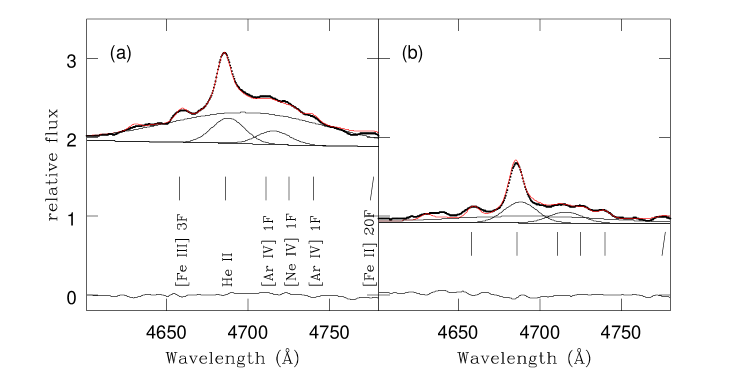
Figure 4: (a) Fit of the mean of the four strongest spectra of Mark 110 in the region around He II $\lambda$4686 and He I $\lambda$4713. The dotted line shows the observations; the continuous line is the best fit. The lowest line represents the residuals. We also show the three He I and He II variable components. The locations of the strongest narrow lines are indicated. (b) The same for the mean of the four weakest spectra.

If the BLR is a rotating disk, the observed line width depends on its inclination to the line of sight. Collin & Kawaguchi (collin04 (2004)) have shown that the BLR should be a geometrically thick disc. Such a disc must be sustained vertically by a turbulent pressure corresponding to a turbulent velocity which is such that, when seen face-on, the width of the emission lines emitted by the disc is reduced compared to an edge-on disc depending on the aspect ratio of the disc h/r. This could cause a systematic underestimation of the central mass by a factor of (h/r)² (Krolik krolik01 (2001)). Accordingly, Kollatschny (2003b ) noted that the derived BH mass is a lower limit. He showed that the redshift of the r.m.s. profiles with respect to the narrow emission lines increases as a function of line width and ionization potential. He interpreted this effect as being due to gravitational redshifts. The BH mass needed to explain these redshifts is M_BH=(14$\pm$3$)\times$10⁷ M$\odot$, implying a value of the aspect ratio smaller than 0.36. We note however that, according to Kollatschny (2003b ), the broadest line, with the largest redshift, is He II $\lambda$4686. But the broad variable emission feature at $\sim$4700 Å which was considered by Kollatschny as being a single very broad He II $\lambda$4686 component is modeled here, ignoring the non variable narrow lines, with three individual broad variable lines: He I $\lambda$ 4713 and He II $\lambda$4686 in the system B3 and He II $\lambda$4686 in the system B1 (Fig. 4). It turns out that the very broad He II line is not always the main contributor to the emission complex and is even barely detected in the 12 weakest spectra. In these conditions it seems doubtful that cross correlating the integrated flux of the broad emission feature with the intensity of the continuum can lead to a reliable timelag.

Müller & Wold (muller06 (2006)), modelling the emission lines emitted near a Kerr BH, have shown that the broad lines observed in Mark 110 could indeed be gravitationally redshifted in an accretion disk having an inclination of $\sim$30°. Moreover, a broad ($\sim$16 200 km s^-1 FWHM), redshifted (z=0.023) component of the O VII triplet (at $\sim$570 eV) discovered in the spectrum of Mark 110 could be due to a gravitational redshift effect; however, infall motion towards the central BH cannot be excluded (Boller et al. boller07 (2007)).

This BH mass ((14$\pm$3$)\times$10⁷ M$\odot$) is about 50 times larger than the value obtained from the bulge velocity dispersion which is unaffected by orientation effects but which could be influenced by the merging experienced by the host galaxy. It is also $\sim$7 times greater than the mass derived from reverberation mapping, but this difference could be explained, as we have seen, if the accretion disk is seen nearly pole-on with an aspect ratio smaller than 0.36.

Papadakis (papadakis04 (2004)) has found a significant anticorrelation between the 2-10 keV variability amplitude and the BH mass. The upper limit observed for the variance of Mark 110 suggests that the BH mass is larger than 10⁷ M$\odot$ (O’Neill et al. oneill05 (2005)), in agreement with the reverberation mapping determination.

5.3 Nature of Mark 110: NLS1 or BLS1?

Subtracting the narrow H$\beta$ components from the average spectrum of Mark 110, we found that the broad emission line system has a width of $\sim$ 1 700 km s^-1 (FWHM) and, therefore, this galaxy could be classified as a NLS1 as suggested by Grupe et al. (grupe04b (2004)). However, this object has none of the other properties characteristic of NLS1s.

NLS1s generally have a soft X-ray excess together with an unusually steep 2-10 keV power law which could be due to a high accretion rate (Pounds et al. pounds95 (1995); Shemmer et al. shemmer06 (2006)), although strong ultra soft X-ray emission is not a universal characteristic of NLS1s (Williams et al. williams04 (2004)). Wang & Netzer (wang03 (2003)) presented a model consisting of an extreme slim disc with a hot corona to explain the soft X-ray excess and suggested that it is a natural consequence of super Eddington accretion.

The X-ray photon index of Mark 110 in the energy range 0.2-2.0 keV ($\Gamma$=2.41$\pm$0.03, Lawrence et al. lawrence97 (1997) or $\Gamma$=2.47$\pm$0.01, Grupe et al. grupe01 (2001)) is typical of BLS1s rather than of NLS1s (Lawrence et al. lawrence97 (1997)) suggesting that this object is not super Eddington (Grupe grupe04 (2004)). Dasgupta & Rao (dasgupta06 (2006)) found $\Gamma$=1.75$\pm$0.01 in the 2-12 keV range and a large soft excess which can be fitted with a blackbody with kT=100$\pm$2 eV. Alternatively, they could fit the data in the range 0.3-12 keV with a broken power law, the values of the photon indices being $\Gamma$=2.29$\pm$0.01 and $\Gamma$=1.78$\pm$0.01 and the break energy 1.66$\pm$0.04 keV. This low value of the 2-12 keV photon index is again typical of BLS1s (Leighly leighly99 (1999), Middleton et al. middleton07 (2007)).

Xu et al. (xu07 (2007)) have shown that, while in NLS1s the electron density of the NLR, as estimated from the [S II]$\lambda$6716/$\lambda$6731 line ratio, covers a rather large range (2-770 cm^-3, corresponding to $\lambda$6716/$\lambda$6731 in the range 0.94-1.23), in BLS1s the density is always relatively large ($>$140 cm^-3, $\lambda$6716/$\lambda$6731 $<$1.27). In Mark 110, we have measured $\lambda$6716/$\lambda$6731=1.12 which does not exclude the possibility that this object is an NLS1 but makes its classification as a BLS1 more likely.

Fe II emission in the broad line region has not been detected and is extremely weak (see above). Boroson (boroson02 (2002)) and Grupe (grupe04 (2004)) suggested that the inverse correlation between the strengths of Fe II and [O III] is driven predominantly by the Eddington ratio. Objects with a high Edington ratio have strong Fe II emission. The extreme weakness of Fe II in Mark 110 therefore also argues for a low Eddington ratio.

If Mark 110 has a relatively low Eddington ratio, its BH mass should be larger than the typical value obtained for NLS1s of similar luminosity.

The Eddington luminosity is taken to be L_Edd=1.25$\times$M_BH/M$\odot$$\times$10³⁸ erg s^-1 (Laor et al. laor97 (1997)) i.e., for Mark 110, 17.4$\times$10⁴⁵ erg s^-1, assuming M_BH=14$\times$10⁷ M$\odot$. The optical luminosity $\lambda$$\times$L_λ at 5100 Å is found to vary in the range (0.11-0.25)$\times$10⁴⁴ erg s^-1 (Peterson et al. peterson98 (1998); Kaspi et al. kaspi05 (2005)) after removal of the host galaxy contribution (Bentz et al. bentz06 (2006)). In these conditions, the bolometric luminosity varies in the range (0.11-0.25)$\times$10⁴⁵ erg s^-1 which corresponds to an Eddington ratio in the range (0.6-1.4)$\times$10^-2. If this is the case, Mark 110 would be far from emitting at the Eddington luminosity. Even if the BH mass is much smaller (e.g. 0.33$\times$10⁷ M$\odot$), the Eddington ratio would be in the range 0.25-0.60, still smaller than one.

5.4 Comparison of Mark 110 with I Zw 1 and IRAS 07598+6508

Mark 110 is the third narrow line Seyfert 1 galaxy for which we have performed a detailed analysis of the emission line spectrum using high signal to noise spectra. The first two were I Zw 1 (Véron-Cetty et al. veron04 (2004)) and IRAS 07698+6508 (Véron-Cetty et al. cetty06 (2006)). These three objects have been classified as NLS1s on the basis of the width of their broad emission lines. Their spectra are extremely dissimilar (Fig. 5).

Figure 5: Spectra of three NLS1s. Fluxes are in units of 10^-15 erg s^-1 cm^-2 Å^-1. As shown in the text, although Mark 110 has narrow ”broad” emission lines, it is probably not a genuine NLS1.

IRAS 07598+6508 is a very strong Fe II emitter with R₄₅₇₀=Fe II $\lambda$4570/H$\beta$$\sim$8. The spectrum is completely dominated by broad permitted lines of Fe II, Ti II and Cr II. No narrow line could be detected. In I Zw 1, the broad permitted Fe II lines are weaker (R₄₅₇₀=1.5-1.9). The narrow line system is relatively weak and is dominated by Fe II permitted and forbidden lines. In Mark 110, no broad Fe II lines could be detected while the narrow line system is much stronger relative to the broad lines.

Vestergaard & Peterson (vestergaard06 (2006)) have determined the luminosity of the nucleus and the BH mass of I Zw 1. They found $\lambda$$\times$L(5100)= 6.22$\times$10⁴⁰ erg s^-1 and M_BH=2.65$\times$10⁷ M$\odot$ which leads to an Eddington ratio of 1.8.

The flux density of IRAS 07598+6508 at 5100 Å is 3.64$\times$10^-16 erg s^-1 cm^-2 Å^-1 which, with z= 0.149, corresponds to $\lambda$$\times$L(5100)=8.9$\times$10⁴⁴ erg s^-1. According to Bentz et al. (bentz06 (2006)) this corresponds to a size of the broad line region of 100 l.d. Then, according to Kaspi et al. (kaspi05 (2005)) and using k=1.26 and 1 780 km s^-1 for the H$\beta$ FWHM (Véron-Cetty et al. veron01 (2001)), the BH mass is M_BH=7.34$\times$10⁷ M$\odot$. We deduced from these numbers that the Eddington ratio is equal to $\sim$1.

The values of the Eddington ratio for these three galaxies are quite uncertain but seem to confirm that this is an important parameter in determining the main properties of the emission line spectrum of this type of object.

5.5 Other similar objects

Kaz 320 is a Seyfert 1 galaxy (B=13.8) at z=0.034. The FWHM of the broad H$\beta$ component is equal to 1 375 km s^-1 (Botte et al. botte04 (2004)) or 1 470 km s^-1 (Véron-Cetty et al. veron01 (2001)). The spectrum exhibits strong Balmer and [O III] lines together with some highly ionized species like [Fe VII]$\lambda$6087 and [Fe X]$\lambda$6375. According to Zamorano et al. (zamorano92 (1992)), permitted Fe II lines, if present, are too weak to be detected. However we have measured R₄₅₇₀=0.49. We found that the H$\beta$ FWHM of the broad component is equal to 1 470 km s^-1 (Véron-Cetty et al. veron01 (2001)).

HS 0328+0528 is a Seyfert 1 galaxy (B=15.7) at z=0.043 (Perlman et al. perlman96 (1996); Engels et al. engels98 (1998)). The FWHM of the broad Balmer component is $\sim$1 500 km s^-1. The Fe II emission is weak (R₄₅₇₀=0.43)(Véron-Cetty et al. veron01 (2001)).

The BH mass has been estimated to be 0.23 and 0.53$\times$10⁷ M$\odot$ respectively in these two objects (Wang & Lu wang01 (2001)). Like Mark 110, they could be pole-on, but otherwise normal BLS1s.

6 Conclusion

We have analyzed the optical emission line spectrum of the peculiar NLS1 galaxy Mark 110. Except for ”narrow” broad lines, Mark 110 lacks all other characteristics of this class of objects such as a weak [O III]$\lambda 5007$/H$\beta$ ratio and strong permitted Fe II lines (We have shown that all the detected Fe II lines belong to the narrow line system). The X-ray spectrum of Mark 110 is also more similar to that of a BLS1 than that of an NLS1.

The properties of the NLS1s are generally attributed to a high accretion rate on a relatively small mass BH leading to a super Eddington luminosity. We argue that, although the ”broad” emission lines in Mark 110 are narrow ($\sim$1 700 km s^-1), its BH mass is such that its luminosity is not super Eddington.

The analysis of the narrow line system indicates that the electron density fills the range 10³ - 10⁶ cm^-3 with a column density between 5$\times$10¹⁹ and 5$\times$10²¹ cm^-2.

The broad lines have three components with a FWHM of 6 000, 3 340 and 1 515 km s^-1 respectively. The first and the third components are variable while, strangely, the second is not.

Comparison with two previously studied NLS1s (IRAS 07598+6508 and I Zw 1) shows the diversity of the emission spectrum of these objects which exhibit a very large range of Fe II emission intensity. The total width of the broad lines, although easy to measure, is probably not a major significant physical parameter to classify these objects. The Eddington luminosity, much more difficult to evaluate, is certainly more important.

We note that a few other objects such as Kaz 320 and HS 0328+0528, are similar to Mark 110 in having ”narrow” broad lines, but weak Fe II and strong [O III], constituting a sub-class of BLS1s with ”narrow” broad lines.

7 Acknowledgments

We gratefully thank M.C. Bentz who kindly put at our disposal her HST image of Mark 110 and S. Collin and D. Péquignot for helpful discussions. We acknowledge the referee, D. Grupe, thanks to whom the paper has been significantly improved.

Appendix A Line list for the narrow line region

Table 5: Lines observed in the stronger narrow line system. Col. 1 : line identification, col. 2 : rest wavelength, col. 3 : intensity relative to H$\beta$ (H$\beta$ flux = 20.3$\times$10^-15 erg s^-1 cm^-2).

Name	wavelength	intensity
H$\beta$	4861.33	1.00
H$\alpha$	6562.77	3.02
H$\gamma$	4340.47	0.48
Ti II 33	4227.34	0.04
$\rm[FeII]$ 21F	4231.56	0.00
Fe II 27	4233.17	0.02
Cr II 31	4233.25	0.02
Cr II 17	4238.69	0.03
$\rm[FeII]$ 21F	4243.97	0.10
$\rm[FeII]$ 21F	4244.81	0.02
$\rm[FeII]$ 21F	4276.83	0.06
$\rm[FeII]$ 7F	4287.39	0.09
$\rm[FeII]$ 21F	4305.90	0.02
$\rm[FeII]$ 21F	4319.63	0.04
He II 3	4338.67	0.01
$\rm[FeII]$ 21F	4346.85	0.02
$\rm[FeII]$ 21F	4352.78	0.03
$\rm[FeII]$ 21F	4358.36	0.04
$\rm[FeII]$ 7F	4359.33	0.07
$\rm[OIII]$ 2F	4363.21	0.77
Ti II 104	4367.66	0.10
$\rm[FeII]$ 21F	4372.43	0.02
Ti II 93	4374.82	0.04
He I 51	4387.93	0.00
$\rm[FeII]$ 7F	4413.78	0.05
$\rm[FeII]$ 6F	4416.27	0.05
$\rm[FeII]$ 6F	4432.45	0.00
Ti II 19	4443.80	0.01
$\rm[FeII]$ 7F	4452.10	0.03
$\rm[FeII]$ 6F	4457.94	0.02
He I 14	4471.69	0.05
$\rm[FeII]$ 7F	4474.90	0.02
Mg II 4	4481.13	0.03
Ti II 115	4488.32	0.02
$\rm[FeII]$ 6F	4488.75	0.01
Fe II 37	4489.18	0.01
Fe II 37	4491.40	0.03
$\rm[FeII]$ 6F	4492.63	0.01
Ti II 31	4501.27	0.06
Fe II 38	4508.28	0.05
$\rm[FeII]$ 6F	4509.60	0.00
$\rm[FeII]$ 6F	4514.90	0.01
Fe II 37	4515.34	0.05
Fe II 37	4520.22	0.02
Fe II 38	4522.63	0.03
$\rm[FeII]$ 6F	4528.38	0.00
Ti II 82	4529.46	0.02
$\rm[FeII]$ 6F	4533.00	0.00
He II 2	4541.49	0.05
Fe II 38	4549.47	0.04
Fe II 37	4555.89	0.02
Cr II 44	4558.68	0.03
Ti II 50	4563.76	0.03
Ti II 81	4571.97	0.03
Fe II 38	4576.33	0.03
Fe II 37	4582.83	0.01

Table 5: (continued)

Name	wavelength	intensity
Fe II 38	4583.83	0.04
Ti II 50	4589.96	0.04
Fe II 38	4620.51	0.00
Fe II 37	4629.34	0.03
$\rm[FeII]$ 4F	4639.67	0.00
?	4642.78	0.02
$\rm[FeIII]$ 3F	4658.05	0.05
$\rm[FeII]$ 4F	4664.44	0.00
He II 1	4685.68	0.22
$\rm[ArIV]$ 1F	4711.37	0.01
He I 12	4713.17	0.00
$\rm[NeIV]$ 1F	4714.25	0.02
$\rm[NeIV]$ 1F	4715.61	0.01
$\rm[NeIV]$ 1F	4724.15	0.02
$\rm[NeIV]$ 1F	4725.62	0.02
$\rm[FeII]$ 4F	4728.07	0.01
Fe II] 43	4731.45	0.02
$\rm[ArIV]$ 1F	4740.16	0.04
$\rm[FeII]$ 4F	4772.06	0.00
$\rm[FeII]$ 20F	4774.72	0.01
$\rm[FeII]$ 4F	4798.27	0.00
$\rm[FeII]$ 20F	4814.53	0.05
Cr II 30	4824.13	0.02
$\rm[FeII]$ 20F	4874.48	0.01
$\rm[FeII]$ 20F	4905.34	0.02
He I 48	4921.93	0.01
Fe II 42	4923.92	0.05
$\rm[FeIII]$ 1F	4930.53	0.05
$\rm[FeII]$ 20F	4947.38	0.01
$\rm[FeII]$ 20F	4950.74	0.01
$\rm[OIII]$ 1F	4958.91	2.98
$\rm[FeII]$ 20F	4973.39	0.01
$\rm[FeII]$ 20F	5005.51	0.01
$\rm[FeII]$ 4F	5006.65	0.00
$\rm[OIII]$ 1F	5006.84	8.96
He I 4	5015.67	0.02
Fe II 42	5018.43	0.08
$\rm[FeII]$ 20F	5020.23	0.01
$\rm[FeII]$ 20F	5043.52	0.01
$\rm[FeII]$ 18F	5107.94	0.00
$\rm[FeII]$ 19F	5111.63	0.01
$\rm[FeII]$ 18F	5158.00	0.01
$\rm[FeII]$ 19F	5158.78	0.07
$\rm[FeII]$ 35F	5163.95	0.05
Fe II 42	5169.03	0.03
$\rm[FeII]$ 18F	5181.95	0.00
$\rm[ArIII]$ 3F	5191.82	0.03
Fe II 49	5197.57	0.01
$\rm[NI]$ 1F	5197.90	0.01
$\rm[FeII]$ 35F	5199.17	0.01
$\rm[NI]$ 1F	5200.26	0.04
$\rm[FeII]$ 19F	5220.06	0.01
Fe II 49	5234.62	0.03
$\rm[FeII]$ 19F	5261.62	0.04
$\rm[FeII]$ 18F	5268.88	0.00
$\rm[FeIII]$ 1F	5270.40	0.03
$\rm[FeII]$ 18F	5273.35	0.01
Fe II 49	5275.99	0.03

Table 5: (end)

Name	wavelength	intensity
$\rm[FeII]$ 35F	5278.37	0.01
$\rm[FeII]$ 35F	5283.11	0.01
?	5288.90	0.02
$\rm[FeII]$ 19F	5296.83	0.01
Fe II 49	5316.61	0.04
Fe II 49	5325.56	0.02
$\rm[FeII]$ 19F	5333.65	0.03
Ti II 69	5336.81	0.02
$\rm[FeII]$ 18F	5347.65	0.00
$\rm[FeII]$ 19F	5376.47	0.02
He II 2	5411.52	0.00
$\rm[FeII]$ 17F	5412.65	0.03
Fe II 49	5425.27	0.02
$\rm[FeII]$ 18F	5433.13	0.00
$\rm[FeII]$ 34F	5477.25	0.01
$\rm[FeII]$ 17F	5495.82	0.01
$\rm[FeII]$ 17F	5527.34	0.04
Fe II] 55	5534.86	0.03
$\rm[FeII]$ 18F	5556.31	0.00
$\rm[OI]$ 3F	5577.34	0.01
?	5608.74	0.01
$\rm[FeII]$ 17F	5654.85	0.01
$\rm[FeII]$ 17F	5745.70	0.00
$\rm[FeII]$ 34F	5746.97	0.01
$\rm[NII]$ 3F	5754.57	0.03
$\rm[FeIV]$	5798.78	0.01
$\rm[FeII]$ 34F	5843.90	0.00
He I 11	5875.70	0.10
Na I D	5889.95	0.03
Na I D	5895.92	0.03
$\rm[OI]$ 1F	6300.23	0.60
$\rm[SIII]$ 1F	6312.06	0.07
Si II 2	6347.09	0.02
$\rm[OI]$ 1F	6363.88	0.20
Si II 2	6371.36	0.05
$\rm[NII]$ 1F	6548.04	0.14
He II 2	6560.10	0.02
$\rm[NII]$ 1F	6583.46	0.43
He I 46	6678.15	0.03
$\rm[SII]$ 2F	6716.44	0.58
$\rm[SII]$ 2F	6730.81	0.51
$\rm[FeVII]$ 2F	4893.90	0.01
$\rm[CaVII]$ 1F	4940.30	0.02
$\rm[FeVII]$ 2F	4942.49	0.04
$\rm[FeVI]$ 2F	4967.13	0.06
$\rm[FeVI]$ 2F	4972.47	0.09
$\rm[FeVI]$ 2F	5145.75	0.03
$\rm[FeVII]$ 2F	5158.41	0.09
$\rm[FeVI]$ 2F	5176.04	0.14
$\rm[FeVII]$ 2F	5276.39	0.05
$\rm[FeXIV]$ 1F	5303.60	0.01
$\rm[CaV]$ 1F	5308.90	0.08
$\rm[CaVII]$ 1F	5620.36	0.01
$\rm[FeVI]$ 1F	5631.07	0.01
$\rm[CaVI]$ 2F	5631.40	0.01
$\rm[FeVI]$ 1F	5676.95	0.03
$\rm[FeVII]$ 1F	5720.71	0.13
$\rm[FeVII]$ 1F	6086.30	0.18

References

- (1) Adams, T.F. 1977, ApJS, 33,19
- (2) Appenzeller, I. & Ostreicher, R. 1988, AJ, 95,45
- (3) Arakelyan, M.A., Dibai, E.A., Esipov, V.F. & Markaryan, B.E. 1970, Astrophysics, 6,189
- (4) Barth, A.J., Greene, J.E. & Ho, L.C. 2005, ApJ, 619,L151
- (5) Baskin, A. & Laor, A. 2005, MNRAS, 358,1043
- (6) Bentz, M.C., Peterson, B.M., Pogge, R.W., Vestergaard, M. & Onken, C.A. 2006, ApJ, 644,133
- (7) Bischoff, K. & Kollatschny, W. 1999, A&A, 345,49
- (8) Boller, T., Balestra, I. & Kollatschny, W. 2007, A&A, 465,87
- (9) Boroson, T.A. 2002, ApJ, 565,78
- (10) Boroson, T.A. & Green, R.F. 1992, ApJS, 80,109
- (11) Botte, V., Ciroi, S., Rafanelli, P. & Di Mille, F. 2004, AJ, 127,3168
- (12) Botte, V., Ciroi, S., Di Mille F., Rafanelli, P. & Romano, A. 2005, MNRAS, 356,789
- (13) Collin, S. & Joly, M. 2000, New Astronomy Review, 44,531
- (14) Collin, S. & Kawaguchi, T. 2004, A&A, 426,797
- (15) Cool, R.J., Howell, S.B., Pena, M., Adamson, A.J. & Thompson, R.R. 2005, PASP, 117,462
- (16) Crawford, F.L., McKenna, F.C., Keenan, F.P. et al. 1999, A&AS, 139,135
- (17) Crenshaw, D.M. 1986, ApJS, 62,821
- (18) Dasgupta, S. & Rao, A.R. 2006, ApJ, 651,L13
- (19) De Robertis, M.M. & Osterbrock, D.E. 1984, ApJ, 286,171
- (20) Elvis, A., Wilkes, B.J., McDowell, J.C. et al. 1999, ApJS, 95,1
- (21) Engels, D., Hagen, H.-J., Cordis, L. et al. 1998, A&AS, 128,507
- (22) Feldman, F.R., Weedman, D.W., Balzano, V.A. & Ramsey, L.W. 1982, ApJ, 256,427
- (23) Ferrarese, L. & Merritt, D. 2000, ApJ, 539,L9
- (24) Ferrarese, L., Pogge, R.W., Peterson, B.M. et al. 2001, ApJ, 555,L79
- (25) Garcia-Lario, P., Riera, A. & Manchado, A. 1999, ApJ, 526,854
- (26) Greene, J.E. & Ho, L.C. 2006, ApJ, 641,L21
- (27) Grupe, D. 2004, AJ, 127,1799
- (28) Grupe, D., Beuermann, K., Mannheim, K. & Thomas, H.-C. 1999, A&A, 350,805
- (29) Grupe, D., Thomas, H.-C. & Beurmann, K. 2001, A&A, 367,470
- (30) Grupe D., Wills, B.J., Leighly, K.L. & Meusinger, H. 2004, AJ, 127,156
- (31) Harlaftis, E. 1999, A&A, 346,L73
- (32) Hutchings, J.B. & Craven, S.E. 1988, AJ, 95,677
- (33) Kaspi, S., Smith, P.S., Netzer, H. et al. 2000, ApJ, 533,631
- (34) Kaspi, S., Maoz, D., Netzer, H. et al. 2005, ApJ, 629,61
- (35) Keenan, F.P., Crawford, F.L., Feibelman, W.A. & Aller, L.H. 2001, ApJS, 132,103
- (36) Kollatschny, W. 2003a, A&A, 407,461
- (37) Kollatschny, W. 2003b, A&A, 412,L61
- (38) Kollatschny, W. & Fricke, K.J. 1981, A&A, 146,L11
- (39) Kollatschny, W., Schneider, H., Fricke, K.J. & York, H.W. 1981, A&A, 104,198
- (40) Kollatschny, W., Bischoff, K. & Dietrich, M. 2000, A&A, 361,901
- (41) Kollatschny, W., Bischoff, K., Robinson, E.L., Welsh, W.F. & Hill, G.J. 2001, A&A, 379,125
- (42) Krolik, J.H. 2001, ApJ, 551,72
- (43) Laor, A., Fiore, F., Elvis, M., Wilkes, B.J. & McDowel, J.C. 1997, ApJ, 477,93
- (44) Lawrence, A., Elvis, M., Wilkes, B.J., McHardy, I. & Brandt, N. 1997, MNRAS, 285,879
- (45) Leighly, K.M. 1999, ApJS, 125,317
- (46) McKenty, J.W. 1990, ApJS, 72,231
- (47) Markaryan, B.E. 1969, Astrophysics, 5,206
- (48) McKenna, F.C., Keenan, F.P., Hambly, N.C. et al. 1997, ApJS, 109,225
- (49) Merrill, P. W. 1961, ApJ, 133,503
- (50) Merritt, D. & Ferrarese, L. 2001, ApJ, 547,140
- (51) Meyers, K.A. & Peterson, B.M. 1985, PASP, 97,734
- (52) Middleton, M., Done, C. & Gierlinski, M. 2007, MNRAS (submitted), astro-ph/0704.2970
- (53) Müller, A. & Wold, M. 2006, A&A, 457,485
- (54) Netzer, H. 1990, in: Active galactic nuclei, R.D. Blanford, Netzer, H. & Woltjer, L. eds.
- (55) O’Neill, P.M., Nandra, K., Papadakis, I.E. & Turner, T.J. 2005, MNRAS, 358,1405
- (56) Onken, A., Ferrarese, L., Merritt, D. et al. 2004, ApJ, 615,645
- (57) Osterbrock, D.E. 1974, Astrophysics of gaseous nebulae, W.H. Freeman and company
- (58) Osterbrock, D.E. 1977, ApJ, 215,733
- (59) Osterbrock, D.E. & Pogge, R.W. 1985, ApJ, 297,166
- (60) Papadakis, I.E. 2004, MNRAS, 348,207
- (61) Perlman, E.S., Stocke, J.T., Schachter, J.F. et al. 1996, ApJS, 104,251
- (62) Peterson, B.M. 1988, PASP, 100,18
- (63) Peterson, B.M. & Wandel, A. 2000, ApJ, 540,L13
- (64) Peterson, B.M., Foltz, C.B., Crenshaw, D.M., Meyers, K.A. & Byard, M.C. 1984, ApJ, 279,529
- (65) Peterson, B.M., Crenshaw, D.M. & Meyers, K.A. 1985, ApJ, 298,283
- (66) Peterson, B.M., Wanders, I., Bertram, R. et al. 1998, ApJ, 501,82 (erratum in ApJ, 511,513)
- (67) Peterson, B.M., Ferrarese, L., Gilbert, K.M. et al. 2004, ApJ, 613,682
- (68) Phillips, M.M. 1978, ApJ, 226,736
- (69) Pounds, K.A., Done, C. & Osborne, J.P. 1995, MNRAS, 277,L5
- (70) Schlegel, D.J., Finkbeiner, D.P. & Davis, M. 1998, ApJ, 500,525
- (71) Shemmer, O., Brandt, W.N., Netzer, H., Maiolino, R. & Kaspi, S. 2006, ApJ, 646,L29
- (72) Stepanian, J.A., Benitez, E., Krongold, Y. et al. 2003, ApJ, 588,746
- (73) Storey, P.J. & Zeippen, C.J. 2000, MNRAS, 312,813
- (74) Véron, P., Lindblad, P.O., Zuiderwijk, E.J., Véron-Cetty, M.-P. & Adams, G. 1980, A&A, 87,245
- (75) Véron-Cetty, M.-P., Véron, P. & Goncalves, A.C. 2001, A&A, 372,730
- (76) Véron-Cetty, M.-P., Joly, M. & Véron, P. 2004, A&A, 417,515
- (77) Véron-Cetty, M.-P., Joly, M. & Véron, P. 2006, A&A, 451,851
- (78) Vestergaard, M. & Peterson, B.M. 2006, ApJ, 625,688
- (79) Vrtilek, J.M. & Carleton, N.P. 1985, ApJ, 294,106
- (80) Wandel, A., Peterson, B.M. & Malkan, M.A. 1999, ApJ, 526,579
- (81) Wang, T. & Lu, Y. 2001, A&A, 377,52
- (82) Wang, J.M. & Netzer, H. 2003, A&A, 398,927
- (83) Wang, J., Wei, J.Y. & He, X.T. 2005, A&A, 436,417
- (84) Webb, W. & Malkan, M. 2000, ApJ, 540,652
- (85) Wehinger, P.A. & Wyckoff, S. 1977, MNRAS, 72,231
- (86) Williams, R.J., Mathur, S. & Pogge, R.W. 2004, ApJ, 610,737
- (87) Wu, J.-H., He, X.-T., Chen, Y. & Voges, W. 2003, Chin. J. Astron. Astrophys., 3,423
- (88) Xu, D., Komossa, S., Zhou, H., Wang, T., Wei, J. 2007,ApJ (in press), astro-ph/0706.2574
- (89) Zamorano, J., Gallego, J., Rego, M., Vitores, A.G. & Gonzalez-Riestra, R. 1992, AJ, 104,1000