Spontaneous soliton symmetry breaking in two-dimensional coupled Bose-Einstein condensates supported by optical lattices

Abstract

Models of two-dimensional (2D) traps, with the double-well structure in the third direction, for Bose-Einstein condensate (BEC) are introduced, with attractive or repulsive interactions between atoms. The models are based on systems of linearly coupled 2D Gross-Pitaevskii equations (GPEs), where the coupling accounts for tunneling between the wells. Each well carries an optical lattice (OL) (stable 2D solitons cannot exist without OLs). The linear coupling splits each finite bandgap in the spectrum of the single-component model into two subgaps. The main subject of the work is spontaneous symmetry breaking (SSB) in two-component 2D solitons and localized vortices (SSB was not considered before in 2D settings). Using variational approximation (VA) and numerical methods, we demonstrate that, in the system with attraction or repulsion, SSB occurs in families of symmetric or antisymmetric solitons (or vortices), respectively. The corresponding bifurcation destabilizes the original solution branch and gives rise to a stable branch of asymmetric solitons or vortices. The VA provides for an accurate description of the emerging branch of asymmetric solitons. In the model with attraction, all stable branches eventually terminate due to the onset of collapse. Stable asymmetric solitons in higher finite bandgaps, and vortices with a multiple topological charge are found too. The models also give rise to first examples of embedded solitons and embedded vortices (the states located inside Bloch bands) in two dimensions. In the linearly-coupled system with opposite signs of the nonlinearity in the two cores, two distinct types of stable solitons and vortices are found, dominated by either the self-attractive component or the self-repulsive one. In the system with a mismatch between the two OLs, a pseudo-bifurcation is found: when the mismatch attains its largest value ($\pi$), the bifurcation does not happen, as branches of different solutions asymptotically approach each other but fail to merge.

I Introduction

A great variety of dynamical patterns in Bose-Einstein condensates (BECs) can be supported by optical lattices (OLs), i.e., spatially periodic potentials induced by laser beams illuminating the BEC Markus . A well-known species of such patterns are gap solitons in condensates composed of repulsively interacting atoms. Gap solitons in BEC were predicted theoretically GS -Ostrovskaya2 , and then created in a “cigar-shaped” (i.e., nearly one-dimensional, 1D) crossed-beam optical trap, to which a longitudinal OL was added. In self-attractive media, the OL potential makes it possible to trap a usual soliton at a required position, and generates stable multi-soliton complexes Wang . In the case of a very deep OL, the corresponding Gross-Pitaevskii equation (GPE) Pit reduces to a discrete nonlinear Schrödinger (NLS) equation Smerzi , which supports well-known solitons, including staggered ones Panos .

Another topic which has drawn a great deal of interest, in terms of BEC double-well and nonlinear optics double-well-optics alike, is spontaneous symmetry breaking (SSB) in matter waves or optical beams trapped in settings based on double-well potentials (using the terminology widely adopted in optics double-well-optics , the medium corresponding to each potential well is sometimes called a “core” below). If two parallel “cigar-shaped” traps are strong enough, the system may be described by a pair of one-dimensional GPEs with linear coupling between them we , hence the destabilization of symmetric solitons and spontaneous transition to asymmetric ones in the double cigar-shaped trap, filled with self-attractive condensate, is described in the same way as the formation of asymmetric solitons in the well-studied model of dual-core nonlinear optical fibers dual-core (in nonlinear optics, the SSB of 1D solitons was also studied in dual-core models with non-Kerr nonlinearities, such as quadratic chi2 and cubic-quintic Lior ). On the other hand, if the dual-core BEC waveguide is realized as a set of two parallel finite-width potential troughs, separated by a finite buffer layer, which are embedded in a 2D (horizontal) trap and tightly confined in the transverse (vertical) direction, the SSB in the respective double-core solitons can be examined in the framework of the full 2D GPE (i.e., considering the tunneling across the buffer layer explicitly, rather than approximating it by the linear coupling between the two 1D equations) Michal . Both models predict a subcritical symmetry-breaking bifurcation for solitons in the self-attractive condensate [which means that branches of asymmetric solutions emerge as unstable ones at the SSB point, and originally go backward (for which reason the bifurcation is also called a backward one), but then turn forward, stabilizing themselves at the turning point].

The objective of the present work is to find symmetric, antisymmetric and asymmetric families of 2D BEC solitons, and similar families of localized vortices (alias vortex solitons), in the system built as a stacked pair of “pancake-shaped” traps, each carrying a two-dimensional OL. The traps are linearly coupled by tunneling across the buffer layer separating them. This model is a natural extension of a double-trap system recently studied in the 1D setting we (in optics, spontaneous symmetry breaking in 1D multi-component gap solitons was studied in models of dual-core Mak and triple-core Arik fiber Bragg gratings). The generalization to the higher dimension is significant, because 2D solitons are drastically different from their 1D counterparts review , especially in the case of the self-attractive nonlinearity (the existence of the respective 2D solitons is fundamentally restricted by the possibility of collapse). Besides that, the new species of vortex solitons is possible in 2D geometry review . To the best of our knowledge, SSB in 2D solitons or vortices has never been considered before.

We will examine different physically relevant versions of the model, with attractive or repulsive nonlinearity in each trap (following Ref. we , they are referred to as AA and RR systems, i.e., “attractive-attractive” and “repulsive-repulsive”). In the AA system, the solitons originate in the semi-infinite gap of the linear spectrum, while in the RR system one may expect to find solitons in finite bandgaps induced by the OL (we will consider the first two gaps, each of them being split into two subgaps under the action of the linear coupling between the traps). In some cases (similar to what was found in the 1D model we ), families of solitons and vortices extend across Bloch bands separating the (sub)gaps, thus becoming embedded solitons embedded . As a matter of fact, the present paper reports the first examples of 2D embedded solitons (and vortices).

A mixed (AR) system, with self-attraction in one trap and self-repulsion in the parallel one, will be considered too. As is known, the sign of the interaction between atoms can be reversed by means of the Feshbach resonance imposed by external magnetic field Feshbach ; accordingly, the signs may be made opposite in the two traps by applying the magnetic field which is inhomogeneous across the “pancake” stack. Solitons in 1D settings of the latter type, but without OLs, were elaborated in Refs. Valery ; a 2D generalization was considered too (with no OLs either) Valery2 , but it does not give rise to stable solitons.

In the normalized form, 2D models considered in this work are based on a system of linearly coupled GPEs for the mean-field wave functions in the two flat traps, $\psi(x,y,t)$ and $\phi(x,y,t)$,

$$i\psi_{t}+\nabla^{2}\psi+\varepsilon\left[\cos(2x)+\cos(2y)\right]\psi+\lambda_{1}|\psi|^{2}\psi+\kappa\phi = 0,$$

$$i\phi_{t}+\nabla^{2}\phi+\varepsilon\left[\cos(2x+\Delta_{1})+\cos(2y+\Delta_{2})\right]\phi+\lambda_{2}|\phi|^{2}\phi+\kappa\psi = 0,$$

where $$x y \nabla^{2} \equiv\partial^{2}/\partial x^{2}+\partial^{2}/\partial y^{2} \lambda_{1,2}=+1 -1 \kappa \varepsilon \pi x y \Delta_{1} \Delta_{2} \Delta_{1}=\Delta_{2}=0 \Delta_{1}=\Delta_{2}=\pi \Delta_{1}=\pi \Delta_{2}=0$$ and are planar coordinates, , and correspond to the attractive and repulsive nonlinearity in the cores, real linear-coupling coefficient is proportional to the rate of tunneling across the potential barrier separating the parallel traps (“cores”), and is the strength of the OLs, whose period is scaled to be . We assume equal depths of the OLs in both traps, while asymmetry between the lattices may be introduced by mismatches (phase shifts) in the - and -directions, and . We will chiefly deal with the symmetric system, i.e., ; nevertheless, effects produced by the mismatches will be addressed too (in fact, we will consider the case of the largest possible mismatch in the diagonal or horizontal direction, i.e., , or , , respectively). In optical models, various effects of the mismatch between linearly-coupled Bragg gratings on gap solitons supported by the gratings were studied in Refs. Yossi .

The 2D form of Eqs. (LABEL:the_model_2d) implies that the “pancake”-shaped traps are tightly confined in the transverse ($Z$) direction, which allows one to reduce the underlying 3D GPE to two dimensions, as performed, in the general form, in Refs. 3D-2D . Together with normalizations of the OL period and nonlinearity constants adopted in Eqs. (LABEL:the_model_2d), this implies that variables $t$ and $\left(x,y\right)$ in Eqs. (LABEL:the_model_2d) are related to physical time $T$ and coordinates $\left(X,Y\right)$ by

$$t\equiv\frac{\pi^{2}\hslash}{2md^{2}}T,~{}\left(x,y\right)\equiv\frac{\pi}{d}\left(X,Y\right),$$ (2)

where $m$ is the atomic mass, and $d$ the OL period in physical units, while the scaled wave functions are related to their counterparts, $\Psi$ and $\Phi$, in the 3D space as follows:

$$\left\{\begin{array}[]{c}\Psi(X,Y,Z,T)\\ \Phi(X,Y,Z,T)\end{array}\right\}=\frac{1}{2}\sqrt{\frac{\pi}{\left|a_{s}\right|d^{2}}}\left\{\begin{array}[]{c}\psi(x,t)\\ \phi(x,t)\end{array}\right\}\exp\left(-\frac{i}{2}\omega_{\perp}T-\frac{m\omega_{\perp}}{2\hbar}Z^{2}\right).$$ (3)

Here $\omega_{\perp}$ is the transverse trapping frequency, and $a_{s}$ the $s$-wave scattering length of atomic collisions ($a_{s}<0$ for attractive interactions). Due to the normalizations, the lattice strength is represented by $\varepsilon=2\mathcal{E}/\mathcal{E}_{\mathrm{rec}}$, where $\mathcal{E}_{\mathrm{rec}}=\left(\pi\hslash\right)^{2}/\left(md^{2}\right)$ is the lattice recoil energy, and $\mathcal{E}$ the depth of the periodic potential in physical units.

The AA and RR systems may be experimentally realized in ⁷Li Lithium or ⁸⁵Rb Cornish , and ⁸⁷Rb Markus condensates, respectively. In this work, the analysis is presented in the range of $\kappa\sim 1$ in Eqs. (LABEL:the_model_2d). With regard to Eqs. (2), the corresponding normalized tunnel-coupling time, $t_{\mathrm{coupl}}=\pi/(2\kappa)$, translates, for $d\sim 1$ $\mu$m, into physical time $T_{\mathrm{coupl}}\sim 10$ $\mu$s and $100$ $\mu$s, for lithium and rubidium, respectively. A prediction most essential to the experiment is the number of atoms expected in stable solitons. Assuming an experimentally relevant value of the trapping frequency – for instance, $\omega_{\perp}\simeq 2\pi\times 100$ Hz for the rubidium condensate (then, the corresponding transverse-confinement size is estimated to be $\sim 1$ $\mu$m, i.e., comparable to the OL period) – and translating the results reported below into physical units, we conclude that the symmetry-breaking 2D solitons are built of $\sim 10^{3}$ atoms. In vortex solitons, the number of atoms is larger, roughly, by a factor of $10$.

The paper is organized as follows. In Section II, we focus on relevant mathematical formulations, which include the linear spectrum of the coupled system, stationary equations for solitons, and the setting for the variational approximation (VA) describing symmetric and asymmetric solitons in the AA and RR systems. Systematic numerical results for solitons in symmetric AA and RR systems (and comparison with predictions of the VA) are reported in Section III, while Section IV reports numerical results for vortex solitons, in the same systems. Findings for asymmetric systems (of the AR type, as well as ones with mismatched OLs) are collected in Section V. Section VI concludes the paper.

II Formulations: the linear spectrum, stationary equations, and variational approximation

II.1 Linear spectra

Before looking for soliton solutions, it is necessary to identify the system’s spectrum within the framework of the linearized equations. First, we consider the symmetric system, with $\Delta_{1}=\Delta_{2}=0$, and look for solutions with chemical potential $\mu$ as

$$\left\{\psi(x,y,t),\phi(x,y,t)\right\}=\left[\alpha(x,y)\pm\beta(x,y)\right]e^{-i\mu t}.$$ (4)

Substituting this in the linearized version of Eqs. (LABEL:the_model_2d), we arrive at a 2D eigenvalue problem based on the decoupled equations,

$$\nabla^{2}\alpha(x,y)+\varepsilon\left[\cos(2x)+\cos(2y)\right]\alpha(x,y) = -(\mu+\kappa)\alpha(x,y),$$ (5a)

$$\nabla^{2}\beta(x,y)+\varepsilon\left[\cos(2x)+\cos(2y)\right]\beta(x,y) = -(\mu-\kappa)\beta(x,y).$$ (5b)

Each one of these equations is tantamount to the eigenvalue problem for the single GPE with a 2D lattice and effective chemical potential $$\mu^{\prime}=\mu\pm\kappa$$. The spectrum generated by the linearization of the single-component GPE is well known, see Refs. Ostrovskaya and references therein. Figure 1 shows a typical example of the spectrum of the 2D coupled system with the zero mismatch. We observe that the linear coupling in Eqs. (LABEL:the_model_2d) splits the finite gaps of the single-component model BEC into pairs of subgaps, which is similar to what was observed, under the action of the linear coupling, in the 1D counterpart of the present system we .

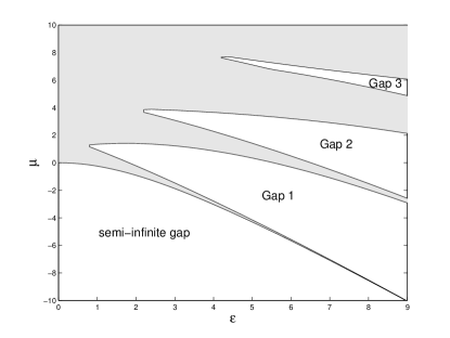
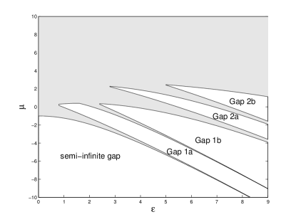
Figure 1: (Color online) The spectrum of the linearized 2D system with aligned optical lattices ($\Delta_{1}=\Delta_{2}=0$). Throughout the paper, all numerically obtained results are given for $\varepsilon=8$, which makes it possible to display the findings in a generic form. Here and in figures following below, Bloch bands are shaded. (a) The uncoupled system, $\kappa=0$; (b) the coupled one, with $\kappa=1$ (unless specified otherwise, all figures in the paper pertain to $\kappa=1$).

To show in detail how the gaps split into subgaps, in Fig. 2 we display the dependence of the chemical potential on vectorial quasi-momentum $\left(k_{x},k_{y}\right)$ in the diagonal direction ($k_{x}=k_{y}\equiv k$), in the uncoupled system and in its coupled counterpart with $\kappa=1$, both pertaining to $\varepsilon=8$. The new, nearly flat, branch of the $\mu(k)$ dependence, which appears in the latter case around $\mu=-7.5$, explains the splitting of former gap 1 into subgaps 1a and 1b by a new very narrow Bloch band, cf. Fig. 1. At other values of $\varepsilon$, the splitting mechanism is quite similar.

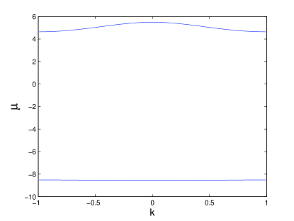
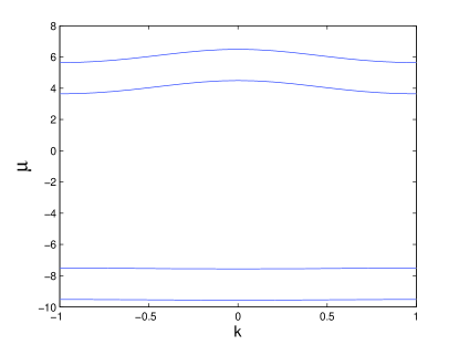
Figure 2: (Color online) The dependence of chemical potential $\mu$ on quasi-momentum $k$ (in the diagonal direction, see text) in the uncoupled system, $\kappa=0$ (a), and in the coupled one, $\kappa=1$ (b). In both cases, $\Delta_{1}=\Delta_{2}=0$ and $\varepsilon=8$. The new nearly flat branch of the dependence, observed around $\mu=-7.5$, explains the splitting of gap 1 into subgaps 1a and 1b in Fig. 1.

Figure 2 and all others in this paper display numerical results for OL strength $\varepsilon=8$ (a moderately deep lattice), which corresponds to the most typical situation. As for coupling constant $\kappa$, the results are displayed for $\kappa=1$ (which also helps to presents generic findings), unless a different value of $\kappa$ is indicated.

As shown in Fig. 3, we also examined the transformation of the linear spectrum under the action of the diagonal mismatch between the OLs in the two traps, assuming $\Delta_{1}=\Delta_{2}\equiv\Delta$. In this case, the linearized equations cannot be decoupled; nevertheless, the computation is straightforward, as we can use the separability of the linear operator to construct eigenfunctions of the 2D model as products of eigenfunctions of the corresponding 1D models we . Figure 3 demonstrates that, with the increase of $\Delta$, the subgaps generated by the coupling-induced splitting tend to shrink, which resembles the trend observed in the 1D model we .

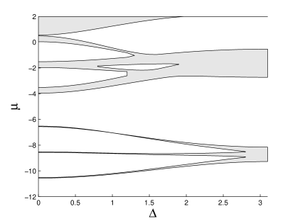
Figure 3: (Color online) The change of the linear spectrum with the increase of diagonal mismatch $\Delta$ between the lattices in the coupled traps, for $\kappa=2$.

II.2 Stationary equations

Stationary solutions to the full nonlinear system of Eqs. (LABEL:the_model_2d) are looked for as $\left\{\psi,\phi\right\}=\left\{u(x,y),v(x,y)\right\}e^{-i\mu t}$, with real functions $u$ and $v$ to be found from equations

$$\mu u+\nabla^{2}u+\varepsilon\left[\cos(2x)+\cos(2y)\right]u+\lambda_{1}u^{3}+\kappa v = 0,$$

$$\mu v+\nabla^{2}v+\varepsilon\left[\cos(2x+\Delta_{1})+\cos(2y+\Delta_{2})\right]v+\lambda_{2}v^{3}+\kappa u = 0.$$

In the symmetric models, i.e., AA and RR ones ($$\lambda_{1}=\lambda_{2}=\pm 1 \Delta_{1}=\Delta_{2}=0 u=v u=-v \mu \hat{u}_{0}(x,y;\mu)$$) with zero mismatch (), symmetric () and antisymmetric () solutions can be expressed in terms of a stationary solution of the single-component GPE with chemical potential , to be denoted as :

$$u(x,y;\mu)=\pm v(x,y;\mu)=\hat{u}_{0}(x,y;\mu\pm\kappa).$$ (7)

Similar to the situation in the 1D model we , we conclude from Eq. (7) that, when the gap splitting occurs, the symmetric and antisymmetric solitons will be moved to the lower and upper subgaps, respectively. In some cases, they may end up in Bloch bands separating the subgaps, thus becoming embedded solitons, examples of which are presented below.

To find general asymmetric soliton solutions and SSB bifurcations linking them to their symmetric and antisymmetric counterparts, we solved the full system of stationary equations (LABEL:stationary_2d) numerically. The stability of all solitons was examined by direct simulations of Eqs. (LABEL:the_model_2d). Soliton families are characterized (see below) by norms of the two components and the total norm,

$$\left\{N_{u},N_{v}\right\}=\int\int\left\{u^{2}(x,y),v^{2}(x,y)\right\}dxdy,~{}N\equiv N_{u}+N_{v},$$ (8)

For asymmetric solutions, we define the asymmetry ratio we as

$$\Theta=\left|N_{u}-N_{v}\right|/\left(N_{u}+N_{v}\right).$$ (9)

The total norm, together with the energy, are dynamical invariants of Eqs. (LABEL:the_model_2d).

II.3 Variational approximation for the symmetric system

The symmetric version of Eqs. (LABEL:stationary_2d) ($\lambda_{1}=\lambda_{2}\equiv\lambda,~{}\Delta_{1}=\Delta_{2}=0$) can be derived from the following Lagrangian:

$$L = \int\int\left[\mu\left(|u|^{2}+|v|^{2}\right)-\left(|\nabla u|^{2}+|\nabla v|^{2}\right)\right.+\varepsilon\left[\cos(2x)+\cos(2y)\right]\left(|u|^{2}+|v|^{2}\right)$$ (10)

$$\left.+\left(\lambda/2\right)\left(|u|^{4}+|v|^{4}\right)+\kappa\left(u^{\ast}v+uv^{\ast}\right)\right].$$

A simple real isotropic Gaussian ansatz Baizakov , with single width $W$ but different amplitudes $A$ and $B$ pertaining to the two components, may be adopted for the solitons:

$$\left(u,v\right)=\left(A,B\right)\exp\left(-\frac{x^{2}+y^{2}}{2W^{2}}\right).$$ (11)

The total norm of this expression is [see Eq. (8)]

$$N=\pi W^{2}\left(A^{2}+B^{2}\right).$$ (12)

The substitution of ansatz (11) in Lagrangian (10) yields the corresponding effective Lagrangian,

$$L_{\mathrm{eff}}/\pi = \mu\left(A^{2}+B^{2}\right)W^{2}-\left(A^{2}+B^{2}\right)+2\varepsilon\left(A^{2}+B^{2}\right)W^{2}e^{-W^{2}}$$ (14)

$$+\left(\lambda/4\right)\left(A^{4}+B^{4}\right)W^{2}+2\kappa ABW^{2}.$$

Variational equations following from this Lagrangian can be conveniently written as

$$\partial L_{\mathrm{eff}}/\partial\left(A^{2}+B^{2}\right)=\partial L_{\mathrm{eff}}/\partial\left(AB\right)=\partial L_{\mathrm{eff}}/\partial\left(W^{2}\right)=0.$$ (15)

For symmetric and antisymmetric solitons, defined by $A=sB$ with $s=\pm 1$, Eqs. (15) amount to a set of two equations,

$$N \equiv 2\pi W^{2}A^{2}=8\pi\lambda\left(1-2\varepsilon W^{4}e^{-W^{2}}\right),$$ (16)

$$\mu+s\kappa = -W^{-2}-2\varepsilon e^{-W^{2}}\left(1-2W^{2}\right).$$ (17)

In the attractive model ($\lambda=+1$), Eqs. (16) and (17) are tantamount to those analyzed in the framework of the VA in Refs. Baizakov and GMM . It was demonstrated that the norm of the 2D soliton takes values in the following intervals:

$$0 < N<N_{\max}^{(\mathrm{attr})}\equiv 8\pi,~{}\mathrm{if~{}}\varepsilon>\varepsilon_{\mathrm{cr}}\equiv e^{2}/8\approx\allowbreak 0.92;$$

$$N_{\min}^{(\mathrm{attr})} \equiv 8\pi\left(1-\varepsilon/\varepsilon_{\mathrm{cr}}\right)<N<8\pi,~{}\mathrm{if~{}}\varepsilon<\varepsilon_{\mathrm{cr}}.$$

Note that $N_{\max}^{(\mathrm{attr})}=8\pi$ corresponds, in terms of the VA Anderson , to the norm of the Townes soliton, i.e., the localized solution of the 2D NLS equation in free space, which is unstable against collapse Berge (while the OL stabilizes 2D solitons Baizakov ; Jianke ). In fact, the vanishing of $N_{\min}^{(\mathrm{attr})}$ at $\varepsilon>\varepsilon_{\mathrm{cr}}$ in Eqs. (LABEL:+1Nmax) is an artifact of the VA Baizakov , explained by the fact that Gaussian ansatz (11) is not appropriate for multi-peaked solitons supported by the strong OL.

In the repulsive model ($\lambda=-1$), variational equations (16) and (17) which, essentially, pertain to the single-component setting, predict solitons only if the OL is strong enough GMM . Indeed, a straightforward consideration of Eq. (16) demonstrates that, in this case, solutions exist only for $\varepsilon>\varepsilon_{\mathrm{cr}}$, the norm of the solution family being limited to interval

$$0<N<N_{\max}^{(\mathrm{rep})}\equiv 8\pi\left(\varepsilon/\varepsilon_{\mathrm{cr}}-1\right)$$ (19)

[$\varepsilon_{\mathrm{cr}}$ is the same as in Eq. (LABEL:+1Nmax)]. The comparison of Eq. (19) with known numerical results for 2D gap solitons Ostrovskaya ; Sakaguchi demonstrates that the nonexistence of solitons in the repulsive model at $\varepsilon<\varepsilon_{\mathrm{cr}}^{(1)}$ is another artifact of the VA, signalling that gap solitons cannot be approximated by simple Gaussian ansatz (11) for $\varepsilon<\varepsilon_{\mathrm{cr}}$.

For asymmetric solitons, with $A^{2}\neq B^{2}$, Eqs. (15) can be cast in the following form:

$$A^{2}+B^{2} = 2\left[\lambda\left(W^{-2}-2\varepsilon W^{2}e^{-W^{2}}\right)+\sqrt{\left(W^{-2}-2\varepsilon W^{2}e^{-W^{2}}\right)^{2}+2\kappa^{2}}\right],$$ (20)

$$AB = 2\lambda\kappa,$$ (21)

$$\mu = -2\varepsilon e^{-W^{2}}\left(1-W^{2}\right)-\lambda\sqrt{\left(W^{-2}-2\varepsilon W^{2}e^{-W^{2}}\right)^{2}+2\kappa^{2}}.$$ (22)

With regard to Eq. (20), norm (12) of the asymmetric solitons becomes

$$N=2\pi\left[\lambda\left(1-2\varepsilon W^{4}e^{-W^{2}}\right)+\sqrt{\left(1-2\varepsilon W^{4}e^{-W^{2}}\right)^{2}+2\kappa^{2}W^{4}}\right],$$ (23)

Variational solutions for the asymmetric solitons are meaningful if they satisfy an obvious condition, $A^{2}+B^{2}\geq 2\left|AB\right|$. In fact, the asymmetric solitons bifurcate from symmetric or antisymmetric ones [if, respectively, $\lambda=+1$ or $-1$, as follows from Eq. (21)] precisely at point $A^{2}+B^{2}=2\left|AB\right|$. Soliton families predicted by the VA, i.e., obtained by numerical solution of Eqs. (20) - (23), are represented by the corresponding dependences $N=N(\mu)$ in Figs. 4 and 7, along with their counterparts found from the numerical solution of full stationary equations (LABEL:stationary_2d).

III Numerical results: solitons

III.1 Symmetric attraction-attraction system

In Fig. 4, we display a generic example of families of antisymmetric, symmetric and asymmetric stationary solitons in the AA model with zero mismatch between the lattices ($\Delta=0$). The families were found from systematic numerical solutions of Eqs. (LABEL:stationary_2d). Figure 4 also includes the solution families as predicted, for the same case, by the VA, which demonstrates good agreement between the variational and numerical results, for all the three types of solitons (at small values of the norm, the variational branches are indistinguishable from their numerical counterparts). A typical example of comparison of the profiles of asymmetric solitons produced by the numerical solution and VA is presented in Fig. 5.

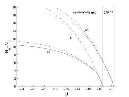
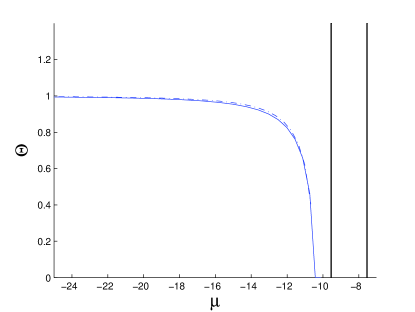
Figure 4: (Color online) Families of 2D solitons found in the symmetric attraction-attraction model ($\lambda_{1}=\lambda_{2}=1$, $\Delta_{1}=\Delta_{2}=0$). Symmetric, antisymmetric and asymmetric solutions are labeled by “s”, “an”, and “as”, respectively. Dashed-dotted lines represent solutions (of all the three types) produced by the variational approximation, while solid and dotted lines depict, respectively, numerically found stable and unstable solutions. (a) The soliton’s total power versus the chemical potential. (b) Ratio $\Theta$ [see Eq. (9)] for the family of asymmetric solitons. The same conventions for labelling solution families of different types (variaitonal/numerical, stable/unstable, symmetric/antisymmetric/asymmetric) are adopted in other figures.

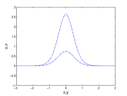
Figure 5: (Color online) Comparison of profiles of the 2D soliton in the attraction-attraction model, as found from the numerical solution and predicted by the variational approximation (solid and dashed curves, respectively). Shown are cross sections of the soliton along $x$- and $y$-axes, for $\mu=-12$. Norms of the two components of the soliton are $N_{u}\approx 4.5$ and $N_{v}\approx 0.4$.

We observe in Fig. 4(a) that the symmetric-soliton branch undergoes a supercritical bifurcation at some critical value of the norm, giving rise to the branch of asymmetric solitons, which is the manifestation of the SSB in this setting (note that the bifurcation point is very accurately predicted by the VA). Symmetric solitons are stable before the bifurcation, and unstable afterwards, while asymmetric solitons emerge as stable solutions [recall the stability of the solutions was identified by direct simulations of Eqs. (LABEL:the_model_2d)]. On the other hand, the family of antisymmetric solitons never bifurcates, i.e., it never gets destabilized through SSB. As a consequence of that, the system features bistability, when the antisymmetric solutions are stable simultaneously with either symmetric or asymmetric ones (below or above the bifurcation point, respectively). It is worthy to note that all branches of the solutions satisfy the Vakhitov-Kolokolov (VK) criterion, $dN/d\mu<0$, which is a necessary stability condition VK ; Berge . It is also noteworthy that the stable branch of antisymmetric solitons displayed in Fig. 4(a) continues across the (narrow) Bloch band separating the semi-infinite gap and subgap 1a. Inside the narrow band, this family represents 2D embedded solitons (which are stable in direct simulations). As far as we know, this is the first example of 2D embedded solitons reported in any model.

The above results resemble findings recently reported in the 1D system we . However, in the 2D case we observe an additional destabilization mechanism in the AA system, through collapse of the soliton of any type, when its norm becomes too large. In particular, the antisymmetric branch, which would be totally stable in the 1D case, loses its stability in the 2D system when the soliton’s norm exceeds the corresponding collapse threshold. Direct simulations demonstrate that, in this situation, the unstable antisymmetric soliton is first transformed into a strongly asymmetric structure; eventually, the high-amplitude component collapses, forming a singularity, while its counterpart with the lower amplitude decays into quasi-linear waves, as shown in Fig. 6.

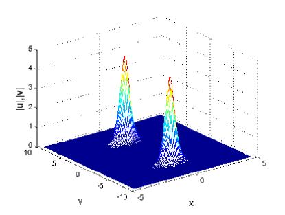
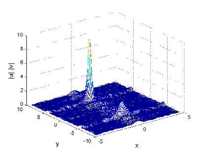
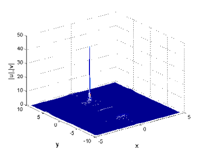
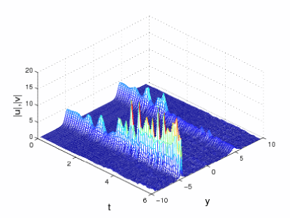
Figure 6: (Color online) Evolution of an antisymmetric 2D soliton (with $\mu=-16$) in the attraction-attraction model, which is destabilized by the collapse. (a) The initial state at $t=0$; (b) the formation of an asymmetric state at $t=4$; (c) the collapse of the high-amplitude component and decay of the low-amplitude one, at $t=6$; (d) the evolution of the entire pattern in the cross section along $x=0$. Here and in similar figures presented below, panels display the side-by-side juxtaposition of the two components, $|u|$ and $|v|$.

The evolution of symmetric solitons destabilized by the SSB bifurcation is not affected by the collapse. Similar to what was reported in the study of the 1D model we , the unstable symmetric solitons clearly tend to rearrange themselves into stable asymmetric counterparts (examples are not shown here, as they are not essentially different from what was observed in the 1D system). The branch of the asymmetric solitons is also subject to the collapse, but this happens on a remote portion of the $N(\mu)$ curve, which could not be shown in Fig. 4.

III.2 Symmetric repulsion-repulsion system

A generic example of families of solitons found in the RR model is shown in Fig. 7. In subgap 1b, the VA predicts the solutions very accurately. For this case, the comparison of numerical and variational asymmetric soliton profiles is displayed in Fig. 8. On the other hand, the VA also predicts asymmetric solutions in subgap 2a, where such solutions could not be found in the numerical form, therefore the extension of the asymmetric branch into the latter subgap is an artifact of the variational method. It is noteworthy too that the stable branch of symmetric solitons crosses the Bloch band separating subgaps 1a and 1b, thus providing for the first example of 2D embedded solitons in a self-defocusing medium. These embedded solitons are stable, as illustrated by an example of the evolution of a perturbed soliton shown in Fig. 9.

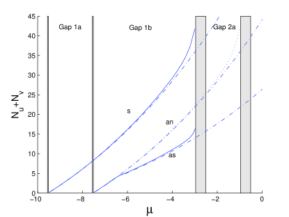
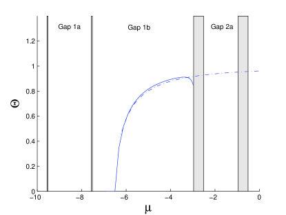
Figure 7: (Color online) The same as in Fig. 4, but for families of solitons in the symmetric repulsion-repulsion model ($\lambda_{1}=\lambda_{2}=-1$, $\Delta=0$). The portion of the asymmetric-soliton branch in subgap 2a is an artifact of the variational approximation.

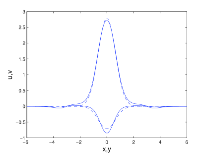
Figure 8: (Color online) Comparison of profiles of asymmetric solitons, as predicted by the VA and found in the numerical form (dashed and solid lines, respectively), in the symmetric repulsive-repulsive model. In this case, $\mu=-4$, and $N_{u}\approx 10.5,N_{v}\approx 0.6.$

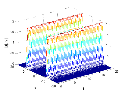
Figure 9: (Color online) Evolution of a perturbed symmetric embedded soliton in the symmetric repulsion-repulsion model is shown in the cross-section along $x=0$. The chemical potential of the unperturbed soliton is $\mu=-7.54$, placing it into the Bloch zone separating subgaps 1a and 1b. The norm of the soliton is $N\approx 8$. The soliton is obviously stable.

The situation in the RR system is closer to what was found for its 1D counterpart in Ref. we (because collapse does not occur with repulsive nonlinearity): the antisymmetric branch undergoes a supercritical bifurcation, which gives rise to stable asymmetric solitons, while the symmetric branch does not bifurcate and remains always stable (the VK criterion does not apply to gap solitons in models with the repulsive nonlinearity). Note that, like in Fig. 4, the bifurcation point is very accurately predicted by the VA. The asymmetric solitons are stable whenever they exist, hence the bistability between symmetric and antisymmetric or asymmetric solitons takes place here. The antisymmetric solitons, destabilized by the SSB bifurcation, transform themselves into persistent localized breathers, see an example in Fig. 10. The breather features oscillations in its two components, with equal amplitudes and phase shift $\pi/2$ between them.

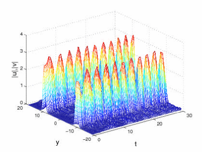
Figure 10: (Color online) Spontaneous transformation of an unstable antisymmetric soliton (with $\mu=-3.5$) into a persistent breather, in the symmetric repulsion-repulsion model ($\lambda_{1}=\lambda_{2}=-1$, $\Delta=0$).

Lastly, stable asymmetric solitons have also been found in higher bandgaps, an example of which is given in Fig. 11. Typically, the solitons in higher bandgaps are less tightly bound, featuring well-pronounced sidelobes.

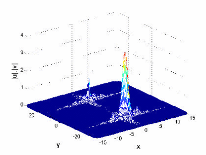
Figure 11: (Color online) An example of a stable asymmetric soliton found, in the symmetric repulsion-repulsion system, in subgap 2a, with $\mu=1$.

IV Numerical results: vortices

IV.1 Symmetric attraction-attraction system

In the model based on the single-component GPE in two dimensions with the OL and attractive nonlinearity, stable solutions in the form of localized vortices with topological charge (“spin”) $S=1$ were reported in Refs. Baizakov and Jianke , and their (also stable) counterparts with $S>2$ were found in Ref. Sakaguchi2 . Before proceeding to the new problem of the SSB in two-component vortices, it is relevant to recapitulate basic results obtained for vortex solitons in the single-component model. Figure 12 shows a generic example of families of vortex-soliton solutions with $S=1$ in this model. The most compact “crater-shaped” vortices, which feature a single peak with a hole in the center, are always unstable. However, the vortices built as 4- and 8-peak complexes, with phase shifts, respectively, $\pi/2$ or $\pi/4$ between the peaks (which corresponds to the net phase circulation of $2\pi$, i.e., $S=1$), constitute entirely stable families (Fig. 12 includes examples of all the three species of localized vortices). These complexes are quite similar to examples of stable vortices reported in Refs. Baizakov and Jianke .

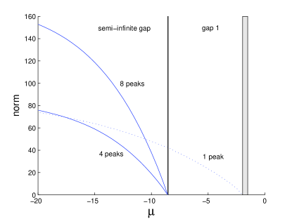
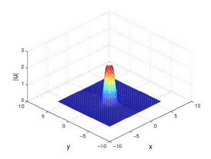
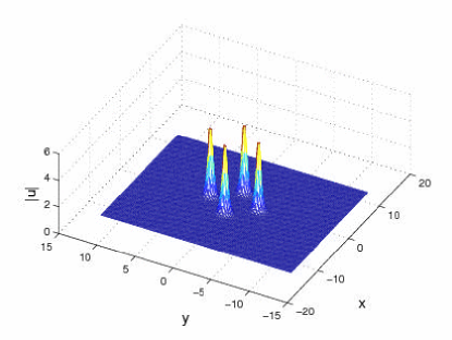
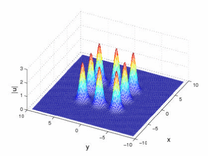
Figure 12: (Color online) Localized vortices with topological charge $S=1$ in the single-component model with attraction ($\lambda=1$). (a) Three solution families (unstable single-peak crater-shaped vortices, and stable 4- and 8-peak vortex complexes) are represented by the dependence of their norm on the chemical potential. (b)-(d) Examples of the three species of localized vortices, with $\left(\mu=-4.5,~{}N\approx 20\right)$, $\left(\mu=-20,~{}N\approx 76\right)$, and $\left(\mu=-12,~{}N\approx 78\right)$, respectively.

We have found the SSB of two-component vortex solitons in the symmetric AA system ($\lambda_{1}=\lambda_{2}=+1$, $\Delta=0$). Families of 4- and 8-peak vortices of the symmetric, antisymmetric and asymmetric types, found in the coupled system, are shown in Figs. 13 and 14, along with examples of respective stable asymmetric vortices.

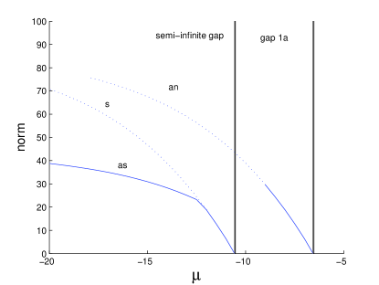
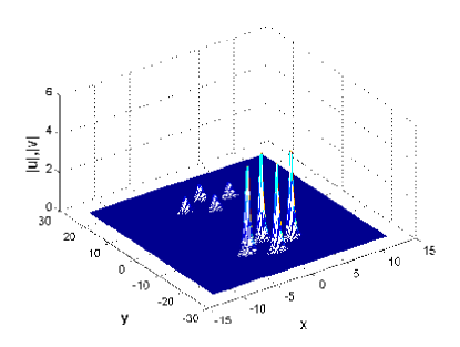
Figure 13: (Color online) 4-peak vortices with topological charge $S=1$, in the symmetric attraction-attraction system, with $\kappa=2$. (a) Families of the symmetric, antisymmetric, and asymmetric vortex solutions represented by $N(\mu)$ curves. (b) An example of a stable asymmetric vortex, for $\mu=-18$ and $N=36.5$.

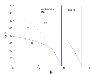
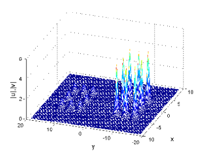
Figure 14: (Color online) The same as in Fig. 13, but for 8-peak vortices. In panel (b), an example of the stable asymmetric vortex is displayed for $\mu=-18$, $N=73.5$.

The stability of these solutions was identified, as above, by direct simulations. Symmetric vortices get destabilized by the bifurcation and tend to spontaneously rearrange into asymmetric ones, which emerge as stable solutions, while antisymmetric vortices do not bifurcate. At large values of the norm, the localized vortices are subject to collapse.

IV.2 Symmetric repulsion-repulsion system

In the repulsive model with the OL, localized vortices may be treated as a species of 2D solitons of the gap type Ostrovskaya2 ; Sakaguchi . First, in Fig. 15 we present families of vortex solitons in the single-component model. Similar to what was shown above for the attractive model, the single-peak (crater-shaped) vortices are unstable, while multiple-peak vortical complexes are stable. However, in the repulsive model only the (unstable) single-peak and (stable) 8-peak structures carry topological charge $S=1$, while the 4-peak entity is a complex bound state of several vortices. Indeed, the phase distribution in the latter state, displayed in Fig. 16, suggests that it may be interpreted as a structure built of of five vortices: one, with $S=1$, is located in the center, being surrounded by four constituent vortices, each carrying charge $S=-1$.

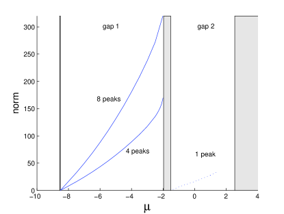
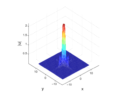
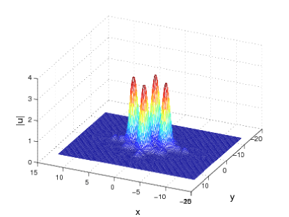
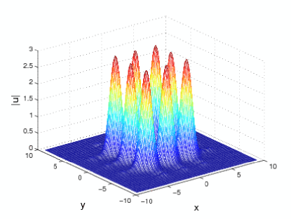
Figure 15: (Color online) Localized vortices in the single-component model with repulsion ($\lambda=-1$). (a) Norm versus the chemical potential for three species of vortex solitons: single-peak, 4-peak, and 8-peak ones. (b)-(d): Examples of vortices of these types, with $\left(\mu=1.5,~{}N\approx 35\right)$, $\left(\mu=-2.5,~{}N\approx 135\right)$, and $\left(\mu=-3.5,~{}N\approx 208\right)$, respectively.

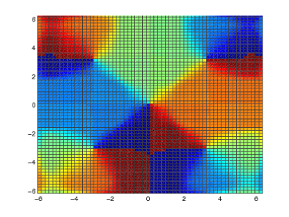
Figure 16: (Color online) The phase pattern in the 4-peak vortex complex in the single-component repulsive model, whose density profile is displayed in Fig. 15(c).

In the coupled (two-component) RR system, we observed SSB in both types of stable vortex states, 4-peak and 8-peak ones, as shown in Fig. 17. Similar to what was demonstrated above for the solitons, the asymmetric branch bifurcates from the antisymmetric one, while the family of the symmetric vortices does not bifurcate and remains entirely stable, thus giving rise to the bistability, together with the stable asymmetric vortices. Antisymmetric two-component vortices destabilized by the SSB bifurcation develop into persistent breathers. A noteworthy feature of Fig. 17 is the fact that the branch of symmetric solutions (both 4- and 8-peak ones) crosses the Bloch band between subgaps 1a and 1b, which provides for the first example of (stable) embedded vortex solitons.

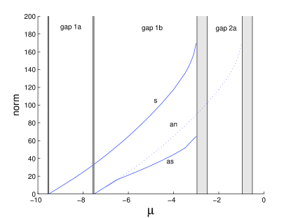
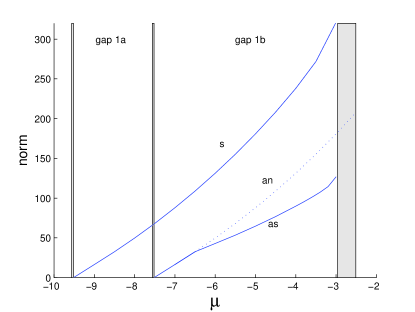
Figure 17: (Color online) Families of 4-peak (a) and 8-peak (b) vortices in the symmetric repulsion-repulsion system.

Stable asymmetric vortices residing in higher bandgaps, as well as stable vortices with higher vorticity, $S>1$, have been found too. In particular, Fig. 18 displays an example of a stable 8-peaked vortex with $S=2$, found in subgap 2a.

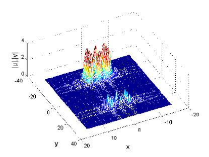
Figure 18: (Color online) A stable asymmetric vortex with topological charge $S=2$, found in the symmetric repulsion-repulsion system. In this case, $\mu=1$ (which falls in subgap 2a). Norms of the components are $N_{u}\approx 272$, $N_{v}\approx 13$. Note the difference in the $x$- and $y$- scales in the figure (in fact, the vortex is invariant with respect to $x\leftrightarrow y$).

V Asymmetric models

As explained in Introduction, the symmetry of coupled equations (LABEL:the_model_2d) may be broken by opposite signs of the nonlinearity in the two cores (in the AR system, with $\lambda_{1}=-\lambda_{2}=+1$), or by mismatches between the lattices in them, $\Delta_{1,2}\neq 0$. We did not aim to perform an exhaustive analysis of the asymmetric models, but examples of stable solitons in these models have been found.

Figure 19 shows stable solitons in the AR system. Solutions of two types have been found in it: one with a dominant self-repulsive component sitting in subgap 1a, and another one with the dominant self-attractive component found, as should be expected, in the semi-infinite gap. Stability of the solitons have been verified by direct simulations.

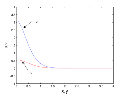
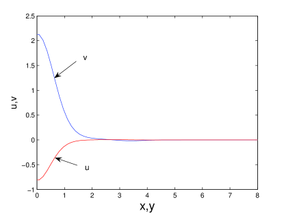
Figure 19: (Color online) Stable solitons in the coupled attraction-repulsion system ($\lambda_{1}=-\lambda_{2}=1,~{}\Delta_{1,2}=0$). The solitons’ profiles are even functions of $x$ and $y$, and are invariant with respect to transformation $x\leftrightarrow y$. (a) A soliton with the dominant self-attractive component. It has $\mu\approx-13$ (which falls in the semi-infinite gap), and $N_{u}\approx 5.7,N_{v}\approx 0.26$. (b) A soliton with the dominant self-repulsive component, found with $\mu\approx-5.7$ (which belongs to subgap 1a) and $N_{u}\approx 0.55,N_{v}\approx 5.35$.

Stable 8-peak vortices with $S=1$ have also been found in the AR model. Vortices with dominant self-attractive and self-repulsive components are located in the semi-infinite gap and subgap 1a, respectively. Their examples are not shown here, as they are very similar to the 8-peak asymmetric solitons found in the AA and RR models, that were reported above.

We have also studied the system with the mismatch between the OLs, concentrating on two most interesting cases, with $\Delta_{1}=\pi,\Delta_{2}=0$ or $\Delta_{1}=\Delta_{2}=\pi$ in Eqs. (LABEL:the_model_2d). In either case, the phase mismatch was given the largest possible value ($\pi$). As in the 1D model with nonzero mismatch we , quasi-symmetric and asymmetric solutions have been identified, as states with $N_{u}=N_{v}$ and $N_{u}\neq N_{v}$, respectively. In the mismatched system, asymmetric solitons have peaks in the two components located at the same position, while in quasi-symmetric solutions the peaks are slightly separated. Typical profiles of quasi-symmetric and asymmetric solutions in the misaligned AA system are shown in Fig. 20 for $\Delta_{1}=\Delta_{2}=\pi$ (this choice corresponds to the largest diagonal mismatch). Direct simulations demonstrate that the quasi-symmetric solitons are always unstable in this case (an explanation of this feature is given below), while the asymmetric solitons are stable, beneath the collapse threshold.

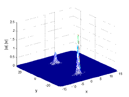
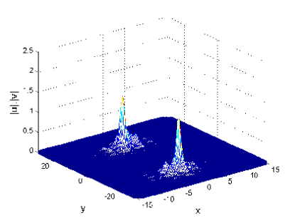
Figure 20: (Color online) Soliton profiles in the attraction-attraction model with the maximum diagonal mismatch between the lattices in the cores, $\Delta_{1}=\Delta_{2}=\pi$, for $\kappa=10$, and $N=5$. (a) A stable asymmetric soliton; (b) an unstable quasi-symmetric soliton.

Further, Fig. 21 depicts the dependence of the asymmetry ratio, defined as per Eq. (9), on coupling coefficient $\kappa$. In the case of the maximum horizontal mismatch, $\Delta_{1}=\pi,\Delta_{2}=0$, we observe that the bifurcation which breaks the (quasi-)symmetry of solitons at a critical value of $\kappa$ is replaced by the pseudo-bifurcation, i.e., the branch of asymmetric solutions asymptotically approaches its quasi-symmetric counterpart with the increase of $\kappa$, but the bifurcation does not happen, since the two branches never merge. A similar phenomenon was reported in the 1D model with $\Delta=\pi$ we . The replacement of the bifurcation by the pseudo-bifurcation is observed only in the case of the largest mismatch, $\Delta_{1}=\pi$ and/or $\Delta_{2}=\pi$, and it explains the above-mentioned total instability of the family of quasi-symmetric solitons, as the corresponding branch never has a chance to get stabilized by the inverse bifurcation (if one considers the evolution of the solutions with the increase of $\kappa$ at fixed total norm $N$).

A new feature specific to the 2D system is that, in the system with the largest diagonal mismatch, $\Delta_{1}=\Delta_{2}=\pi$, the numerical procedure suddenly ceases to converge at some critical value of $\kappa$, and no asymmetric solitons are found past this point. For instance, at $\kappa=15.485$ a stable asymmetric soliton with a regular profile can be found, but when the coupling increases to $\kappa=15.490$, the soliton is lost. The shape of the $\Theta(\kappa)$ dependence in Fig. 21(b) strongly suggests that the branch of asymmetric solitons terminates, in this case, due to a tangent bifurcation, which results from collision and mutual annihilation of the branch with an additional branch of unstable solutions, that we did not aim to find.

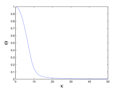
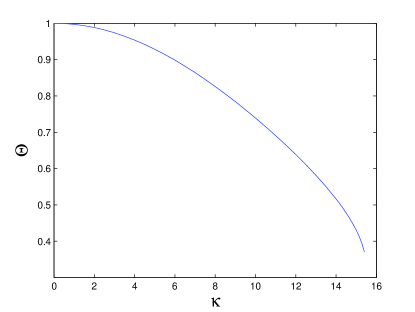
Figure 21: (Color online) The asymmetry ratio, defined as per Eq. (9), as a function of the linear-coupling constant in the misaligned ($\Delta_{1}=\pi,\Delta_{2}=0$) attraction-attraction model with fixed total norm of the two-component soliton, $N=5$. (a) The pseudo-bifurcation. (b) The termination of the family of asymmetric soliton solutions.

Other types of stable solitons and vortices have also been found in the misaligned system of the AA type. In particular, an example of a soliton with two peaks in one component and a single peak in the other is shown in Fig. 22.

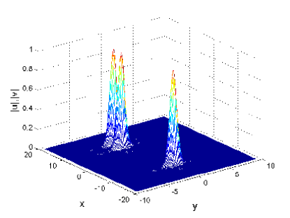
Figure 22: (Color online) A stable soliton in the diagonally mismatched ($\Delta_{1}=\Delta_{2}=\pi$) attraction-attraction system. In this case $\mu=-9$, and $N_{u}=0.8$, $N_{v}=1.6$.

Stable asymmetric solitons in the RR system with misaligned lattices have been found too. A typical stable asymmetric soliton in this system is shown in Fig. 23

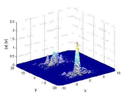
Figure 23: (Color online) An example of a strongly asymmetric stable soliton in the diagonally mismatched ($\Delta_{1}=\Delta_{2}=\pi$) repulsion-repulsion system with $\kappa=10$. This soliton has $\mu=-11$, and $N_{u}=4.4$, $N_{v}=1.6$.

VI Conclusion

We have introduced experimentally relevant models of two stacked flat BEC traps, with attractive or repulsive interactions between atoms. Each flat trap carries an OL (optical lattice), stable 2D solitons being impossible without it. First, it was demonstrated that the linear coupling splits every finite bandgap in the linear spectrum of the single-component model into two subgaps, which are separated by narrow Bloch bands. The main issue, addressed in this work by means of the VA (variational approximation) and numerical methods, is SSB (spontaneous symmetry breaking) in families of solitons and localized vortices, as a result of the competition of three factors: the attractive or repulsive nonlinearity in each core, the action of the OL potential, and the linear coupling between the cores. Similar to what was found in the zero-dimensional setting double-well (this means a double-well potential without any transverse dimension) and one-dimensional models we ; Michal , the SSB occurs in families of symmetric or antisymmetric states, in the case of the attractive or repulsive nonlinearity, respectively. In either case, the corresponding bifurcation destabilizes the branch of symmetric or antisymmetric solitons or vortices, giving rise to a stable branch of asymmetric solutions. The VA, based on the Gaussian ansatz, yields an accurate prediction for the bifurcation and the branch of asymmetric solitons generated by the bifurcation. A feature specific to the 2D setting is the termination of all stable branches in the AA (attraction-attraction) system due to the onset of collapse.

Stable asymmetric solitons sitting in higher finite bandgaps, and localized vortices with multiple values of the topological charge have been found too. In addition, the models considered in this work give rise to first examples of (stable) embedded solitons and embedded vortices (localized states found inside Bloch bands separating the subgaps) in any 2D setting.

Solitons and localized vortices were also considered in the linearly-coupled systems whose symmetry is broken by opposite signs of the nonlinearity in the two traps, or by a mismatch between the OLs in them. In the former case, the system gives rise to two distinct types of stable solitons and vortices, which are dominated by either a self-attractive component or self-repulsive one, which sit, respectively, in the semi-infinite gap, or in a finite bandgap. In the system with mismatched lattices, the phenomenon of the pseudo-bifurcation (which was recently reported in the 1D system we ) was found: when the mismatch takes the largest value ($\pi$) in any direction (horizontal or diagonal), the SSB bifurcation fails to happen, as branches of asymmetric and quasi-symmetric (or quasi-antisymmetric) solutions asymptotically approach each other, but never merge.

This work was supported, in a part, by the Israel Science Foundation through the Center-of- Excellence Grant No. 8006/03 and the German-Israel Foundation (GIF) through Grant No. 149/2006.

References

- (1) O. Morsch and M. Oberthaler, Rev. Mod. Phys. 78, 179 (2006).
- (2) F. Kh. Abdullaev, B. B. Baizakov, S. A. Darmanyan, V. V. Konotop, and M. Salerno, Phys. Rev. A 64, 043606 (2001); I. Carusotto, D. Embriaco, and G. C. La Rocca, ibid. 65, 053611 (2002); B. B. Baizakov, V. V. Konotop and M. Salerno, J. Phys. B 35, 5105 (2002).
- (3) E. A. Ostrovskaya and Y. S. Kivshar, Phys. Rev. Lett. 90, 160407 (2003); 93, 160405 (2004); Opt. Exp. 12, 19 (2004).
- (4) E. A. Ostrovskaya and Y. S. Kivshar, Phys. Rev. Lett. 93, 160405 (2004).
- (5) B. Eiermann, Th. Anker, M. Albiez, M. Taglieber, P. Treutlein, K.-P. Marzlin, and M. K. Oberthaler, Phys. Rev. Lett. 92, 230401 (2004).
- (6) B. A. Malomed, Z. H. Wang, P. L. Chu, and G. D. Peng, J. Opt. Soc. Am. B 16, 1197 (1999); G. L. Alfimov, V. V. Konotop, and M. Salerno, Europhys. Lett. 58, 7 (2002); V. A. Brazhnyi and V. V. Konotop, Mod. Phys. Lett. B 18, 627 (2004).
- (7) F. Dalfovo, S. Giorgini, L. P. Pitaevskii, and S. Stringari, Rev. Mod. Phys. 71, 463 (1999).
- (8) A. Trombettoni and A. Smerzi, Phys. Rev. Lett. 86, 2353-2356 (2001); G. L. Alfimov, P. G. Kevrekidis, V. V. Konotop, and M. Salerno, Phys. Rev. E 66, 046608 (2002).
- (9) P. G. Kevrekidis, K. Ø. Rasmussen, and A. R. Bishop, Int. J. Mod. Phys. B 15, 2833 (2001).
- (10) G. J. Milburn, J. Corney, E. M. Wright, and D. F. Walls, Phys. Rev. A 55, 4318-4324 (1997); A. Smerzi, S. Fantoni, S. Giovanazzi, and S. R. Shenoy, Phys. Rev. Lett. 79, 4950-4953 (1997); J. Ruostekoski and D. F. Walls, Phys. Rev. A 58, R50-R53 (1998); S. Raghavan, A. Smerzi, S. Fantoni, and S. R. Shenoy, ibid. 59, 620-633 (1999); L. Salasnich, A. Parola, and L. Reatto, ibid. 60, 4171-4174 (1999); E. A. Ostrovskaya, Y. S. Kivshar, M. Lisak, B. Hall, F. Cattani, and D. Anderson, ibid. 61, 031601 (2000); J. E. Williams, ibid. 64, 013610 (2001); W. H. Aschbacher , J. Frohlich, G. M. Graf, K. Schnee, and M. Troyer, J. Math. Phys. 43, 3879 (2002); L. Salasnich, A. Parola, and L. Reatto, J. Phys. B - At. Mol. Opt. Phys. 35, 3205 (2002); P. Coullet and N. Vandenberghe, ibid. 35, 1593-1612 (2002); T. G. Tiecke, M. Kemmann, C. Buggle, I. Shvarchuck, W. von Klitzing, and J. T. M. Walraven, J. Opt. B - Quant. Semicl. Opt. 5, S119 (2003); E. Sakellari, N. P. Proukakis, and C. S. Adams, J. Phys. B - At. Mol. Opt. Phys. 37, 3681 (2004); R. K. Jackson and M. I. Weinstein, J. Stat. Phys. 116, 881 (2004); M. Jaaskelainen and P. Meystre, Phys. Rev. A 71, 043603 (2005); E. Infeld, P. Ziń, J. Gocałek, and M. Trippenbach, Phys. Rev. E 74, 026610 (2006); Q.-X. Yuan and G.-H. Ding, Phys. Lett. A 344, 156 (2005); G. Theocharis, P. G. Kevrekidis, D. J. Frantzeskakis, and P. Schmelcher, Phys. Rev. E 74, 056608 (2006); M. Anderlini, J. Sebby-Strabley, J. Kruse, J. V. Porto, and W. D. Phillips, J. Phys. B - At. Mol. Opt. Phys. 39, S199 (2006).
- (11) P. G. Kevrekidis, Z. G. Chen, B. A. Malomed, D. J. Frantzeskakis, and M. I. Weinstein, Phys. Lett. A 340, 275 (2005).
- (12) A. Gubeskys and B. A. Malomed, Phys. Rev. A 75, 063602 (2007).
- (13) W. C. K. Mak, P. L. Chu and B. A. Malomed, J. Opt. Soc. Am. B 15, 1685 (1998); Phys. Rev. E 69, 066610 (2004).
- (14) A. Gubeskys and B. A. Malomed, Eur. Phys. J. D 28, 283 (2004).
- (15) B. A. Malomed, D. Mihalache, F. Wise, and L. Torner, J. Optics B: Quant. Semics. Opt. 7, R53 (2005).
- (16) P. L. Chu, B. A. Malomed, and G. D. Peng, J. Opt. Soc. Am. B 10, 1379 (1993); N. Akhmediev and A. Ankiewicz, Phys. Rev. Lett. 70, 2395 (1993); B. A. Malomed, I. Skinner, P. L. Chu, and G. D. Peng, Phys. Rev. E 53, 4084 (1996).
- (17) W. Mak, B. A. Malomed, and P. L. Chu, Phys. Rev. E 55, 6134 (1997); ibid. 57, 1092 (1998).
- (18) R. Driben, B. A. Malomed, and P. L. Chu, J. Phys. B: At. Mol. Opt. Phys. 39, 2455 (2006); L. Albuch and B. A. Malomed, Mathematics and Computers in Simulation 74, 361 (2007).
- (19) M. Matuszewski, B. A. Malomed, and M. Trippenbach, Phys. Rev. A 75, 063621 (2007).
- (20) J. Yang, B. A. Malomed, and D. J. Kaup, Phys. Rev. Lett. 83, 1958-1961 (1999); A. R. Champneys, B. A. Malomed, J. Yang, and D. J. Kaup, Physica D 152-153, 340 (2001).
- (21) S. Inouye, M. R. Andrews, J. Stenger, H. J. Miesner, D. M. Stamper-Kurn, and W. Ketterle, Nature 392, 51 (1998); E. A. Donley, N. R. Claussen, S. L. Cornish, J. L. Roberts, E. A. Cornell, and C. E. Wieman, ibid. 412, 295 (2001).
- (22) V. S. Shchesnovich, B. A. Malomed, and R. A. Kraenkel, Physica D 188, 213-240 (2004); V. S. Shchesnovich, S. B. Cavalcanti, R. A. Kraenkel, Phys. Rev. A 69, 033609 (2004).
- (23) V. S. Shchesnovich and S. B. Cavalcanti, Phys. Rev. A 71, 023607 (2005); V. S. Shchesnovich and S. B. Cavalcanti, J. Phys. A Math. Gen. 38, 6917 (2005).
- (24) A. A. Sukhorukov and Y. S. Kivshar. Phys. Rev. Lett. 97, 233901 (2006); Y. Tsofe and B. A. Malomed, Phys. Rev. E 75, 056603 (2007).
- (25) L. Salasnich, Laser Phys. 12, 198 (2002); L. Salasnich, A. Parola, and L. Reatto, Phys. Rev. A 65, 043614 (2002); Y. B. Band, I. Towers, and B. A. Malomed, Phys. Rev. A 67, 023602 (2003).
- (26) K. E. Strecker, G. B. Partridge, A. G. Truscott and R. G. Hulet, Nature 417, 150 (2002); L. Khaykovich, F. Schreck, G. Ferrari, T. Bourdel, J. Cubizolles, L. D. Carr, Y. Castin, and C. Salomon, Science 256, 1290 (2002).
- (27) S. L. Cornish, S. T. Thompson, and C. E. Wieman, Phys. Rev. Lett. 96, 170401 (2006).
- (28) B. B. Baizakov, M. Salerno, and B. A. Malomed, Europhys. Lett. 63, 642 (2003); see also an article in Nonlinear Waves: Classical and Quantum Aspects, ed. by F. Kh. Abdullaev and V. V. Konotop, pp. 61-80 (Kluwer Academic Publishers: Dordrecht, 2004; also available at http://rsphysse.anu.edu.au/~asd124/Baizakov_2004_61_NonlinearWaves.pdf).
- (29) A. Gubeskys, B. A. Malomed and I. Merhasin, Stud. Appl. Math. 115, 255 (2005).
- (30) M. Desaix, D. Anderson and M. Lisak, J. Opt. Soc. Am. B 8, 2082 (1991).
- (31) L. Bergé, Phys. Rep. 303, 259 (1998).
- (32) M. G. Vakhitov and A. A. Kolokolov, Sov. J. Radiophys. Quantum Electr. 16, 783 (1973).
- (33) J. Yang and Z. H. Musslimani, Opt. Lett. 28, 2094 (2003).
- (34) H. Sakaguchi and B. A. Malomed, J. Phys. B 37, 2225 (2004).
- (35) H. Sakaguchi and B. A. Malomed, Europhys. Lett. 72, 698 (2005).