Searches for Mixing and $CP$ Violation in the $D^{0}$-$\overline{D}{}^{\,0}$ System

Abstract

We review searches for mixing and $CP$ violation in the $D^{0}$-$\overline{D}{}^{\,0}$ system and discuss the first evidence for mixing recently obtained by the Belle and BABAR collaborations. We also present world average values for the mixing parameters $x=\Delta m/\Gamma$ and $y=\Delta\Gamma/(2\Gamma)$ as calculated by the Heavy Flavors Averaging Group.

I Introduction

Mixing in the $D^{0}$-$\overline{D}{}^{\,0}$ system has been searched for for more than two decades without success — until this past year. Both “$B$-factory” experiments, Belle and BABAR, have recently published evidence for this phenomenon belle_kk ; babar_kpi . Here we review these measurements and discuss their implications. In total four measurements are presented, involving the following decay modes charge_conjugates : $D^{0}\!\rightarrow\!K^{+}\ell^{-}\nu$, $D^{0}\!\rightarrow\!K^{+}K^{-}/\pi^{+}\pi^{-}$, $D^{0}\!\rightarrow\!K^{+}\pi^{-}$, and $D^{0}\!\rightarrow\!K^{0}_{S}\,\pi^{+}\pi^{-}$.

Mixing in heavy flavor systems such as that of $B^{0}$ and $B^{0}_{s}$ is governed by the short-distance box diagram. However, in the $D^{0}$ system this diagram is both doubly-Cabibbo-suppressed and GIM-suppressed relative to the amplitude dominating the decay width, and thus the short-distance rate is very small. Consequently, $D^{0}$-$\overline{D}{}^{\,0}$ mixing is expected to be dominated by long-distance processes that are difficult to calculate; theoretical estimates for the mixing parameters $x\equiv\Delta m/\Gamma$ and $y\equiv\Delta\Gamma/(2\Gamma)$ range over two-three orders of magnitude Petrov . Here, $\Delta M$ and $\Delta\Gamma$ are the differences in the masses and decay widths, respectively, of the two $D^{0}$-$\overline{D}{}^{\,0}$ mass eigenstates, and $\Gamma$ is the mean decay width.

All methods discussed here identify the flavor of the $D^{0}/\overline{D}{}^{\,0}$ when produced by reconstructing the decay $D^{*+}\!\rightarrow\!D^{0}\pi^{+}$ or $D^{*-}\!\rightarrow\!\overline{D}{}^{\,0}\pi^{-}$; the charge of the accompanying pion identifies the $D$ flavor. Because $M_{D^{*}}-M_{D^{0}}-M_{\pi^{+}}\approx 6$ MeV, which is relatively small, the pion has very low momentum and thus is denoted $\pi_{s}$ (“$\pi$ slow”). The $D^{0}$ decay time ($t$) is calculated via $(\ell/p)\times M_{D}$, where $\ell$ is the distance between the $D^{*}$ and $D^{0}$ decay vertices and $p$ is the $D^{0}$ momentum. The $D^{*}$ vertex position is taken to be the intersection of the $\pi_{s}$ momentum with the beamspot profile. Most of the precision on $t$ is due to the vertical ($y$) component of $\ell$, as the spread of the beamspot is only a few microns in this dimension. To reject $D^{(*)}$ decays originating from $B$ decays, one requires $p_{D^{*}}>2.5$ GeV, which is the kinematic endpoint.

II “Wrong-sign” $D^{0}\!\rightarrow\!K^{+}\ell^{-}\nu$ Decays

The decay $D^{0}\!\rightarrow\!K^{+}\ell^{-}\nu$ is in principle an ideal signature for mixing, as this “wrong-sign” (WS) final state can be reached only via a $D^{0}\!\rightarrow\!\overline{D}{}^{\,0}$ transition (in contrast to the “right-sign” (RS) final state $K^{-}\ell^{+}\nu$). However, the neutrino in the final state precludes the decay from being fully-reconstructed, and consequently the decay time measurement is smeared. The decay time dependence is given by $e^{-\Gamma t}[1+(x^{2}+y^{2})t^{2}/2]$, and both Belle and BABAR measure the coefficient $(x^{2}+y^{2})/2\equiv R_{M}$ by fitting the decay time distribution. To reduce backgrounds, only the electron channel ($Ke\nu$) has been used.

Belle uses 253 fb^-1 of data belle_semi , making a relatively loose event selection and fitting the resulting $M(Ke\nu)$ and $\Delta M\equiv M(\pi_{s}\,Ke\nu)-M(Ke\nu)$ distributions to determine the yield of WS events. To improve the resolution on both $\Delta M$ and the decay time, two corrections are made to better determine $P_{\nu}=P_{\rm cms}-P_{\pi Ke}-P_{\rm rest}$, where $P_{\rm rest}$ is the total four-momentum of all tracks and photons in the event besides the $\pi_{s}$, $K$, and $e$ candidates, and $P_{\rm cms}$ is the four-momentum of the center-of-mass (cms) system. First, $P_{\rm rest}$ is rescaled by a factor $x$ such that $(P_{\rm cms}-xP_{\rm rest})^{2}=P^{2}_{D^{*}}=M^{2}_{D^{*}}$; second, $\vec{p}_{\rm rest}$ is rotated in the plane of $\vec{p}_{\rm rest}$ and $\vec{p}_{\pi_{s}Ke}$ such that $(P_{\rm cms}-P_{\pi_{s}Ke}-xP_{\rm rest})^{2}=P^{2}_{\nu}=0$.

The ratio of WS to RS events are measured for six bins of decay time ranging from one to ten $D^{0}$ lifetimes. Summing over all bins, $16430\,\pm 155$ RS and $-1\,\pm 37$ WS events are found. For each bin the ratio depends on $R_{M}$, and the six resulting values of $R_{M}$ are fit to a constant. The result is

$$R_{M} = (0.020\,\pm 0.047\,\pm 0.014)\%\,,$$ (1)

where the first error listed is statistical and the second error is systematic. The latter is dominated by uncertainty in the background $\Delta M$ PDF. As much of the $R_{M}$ likelihood is in the unphysical (negative) region, Belle uses a Feldman-Cousins FeldmanCousins approach to calculate an upper limit; the result is $R_{M}<0.10\%$ at 90% C.L. This limit implies both $|x|$ and $|y|$ are $<4.5$%.

The BABAR experiment uses 344 fb^-1 of data babar_semi and, in contrast to Belle, imposes tight selection criteria to reduce background as much as possible (with a corresponding loss in efficiency). The most restrictive criterion is that events must have a $D^{(*)}$ decay fully reconstructed in the hemisphere opposite that of the semileptonic decay, where the modes $D^{*+}\!\rightarrow\!D^{0}\pi^{+}$, $D^{0}\!\rightarrow\!K^{-}\pi^{+}$, $D^{0}\!\rightarrow\!K^{-}\pi^{+}\pi^{0}$, $D^{0}\!\rightarrow\!K^{-}\pi^{+}\pi^{+}\pi^{-}$, and $D^{+}\!\rightarrow\!K^{-}\pi^{+}\pi^{+}$ are used. This “double-tagging” eliminates copious background from real $D^{0}$’s combining with random $\pi^{\pm}$ tracks to make false $D^{*}$ candidates, but it reduces the signal efficiency by an order of magnitude. The neutrino momentum is determined via a neural network algorithm, and events are required to have decay times in the range 600-3900 fs (corresponding to 1.5-9.5 $D^{0}$ lifetimes). A separate neural network is used to select signal events, and a final set of kinematic selection criteria are applied to the signal side. These criteria include cuts on the $\pi_{s}$ and $e$ momenta, and on the $dE/dx$ of the electron track in the silicon vertex tracker.

The final candidate samples for WS data and Monte Carlo (MC) simulation are shown in Figs. 1a and 1b, respectively. In the data, three events are observed in the signal region $\Delta M<0.20$ GeV/$c^{2}$, whereas the MC predicts (for the luminosity of the data) $2.85\pm 1.43$ background events. Together these values give $R_{M}=(0.004\,^{+0.07}_{-0.06})$%, where the error corresponds to where the log-likelihood function for $N_{s}$ (the true number of signal events) rises by 0.50 units with respect to the minimum value. The points where the log-likelihood function rises by 1.35 units give a 90% C.L. constraint $-0.13\%\!<\!R_{M}\!<\!0.12\%$. This upper bound is similar to the upper limit obtained by Belle.

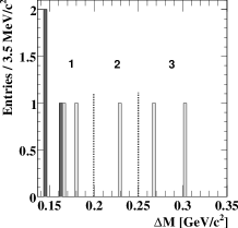
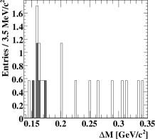
Figure 1: WS $\Delta M$ distribution for BABAR’s $D^{0}\!\rightarrow\!K^{+}\ell^{-}\nu$ candidate sample babar_semi , in data (left) and MC (right). The MC sample is 1.75 times the size of the data sample. The dark (light) histogram shows events after (before) the final kinematic selection. In the left plot, region “1” denotes the signal region used to determine $R_{M}$.

III Hadronic Decays $D^{0}\!\rightarrow\!h^{+}_{1}\,h^{-}_{2}$

Two-body hadronic final states $K^{+}K^{-}$, $\pi^{+}\pi^{-}$, and $K^{\pm}\pi^{\mp}$ can be reached from either $D^{0}$ or $\overline{D}{}^{\,0}$; thus $D^{0}\!\rightarrow\!f$ and $D^{0}\!\rightarrow\!\overline{D}{}^{\,0}\!\rightarrow\!f$ amplitudes both contribute to the decay rate, and detecting the effect of the latter provides evidence for mixing. The time dependence of the decay rate ${\cal R}$ is given by

$$e^{-\Gamma t}\left[1+(y\,{\rm Re}\lambda-x\,{\rm Im}\lambda)t+|\lambda|^{2}\,\frac{x^{2}+y^{2}}{2}\,t^{2}\right]\,,$$ (2)

where $\lambda=(q/p){\cal A}(\overline{D}{}^{\,0}\!\rightarrow\!f)/{\cal A}(D^{0}\!\rightarrow\!f)$ and $q,p$ are complex coefficients relating mass eigenstates to flavor eigenstates: $D_{1,2}=p|D^{0}\rangle\pm q|\overline{D}{}^{\,0}\rangle$. The parameter $\lambda$ can be written $-|q/p||{\cal A}_{\overline{D}{}^{\,0}}/{\cal A}_{D^{0}}|\,e^{i(\phi+\delta)}$, where $\delta$ is the strong phase difference between amplitudes ${\cal A}(\overline{D}{}^{\,0}\!\rightarrow\!f)$ and ${\cal A}(D^{0}\!\rightarrow\!f)$, and $\phi$ is a possible weak phase. In the absence of $CP$ violation ($CPV$), $|q/p|=1$ and $\phi=0$. For $f=K^{-}\pi^{+}$, ${\cal A}(\overline{D}{}^{\,0}\!\rightarrow\!f)$ is doubly-Cabibbo-suppressed, ${\cal A}(D^{0}\!\rightarrow\!f)$ is Cabibbo-favored, and thus $|\lambda|\ll 1$ and ${\cal R}\approx e^{-\Gamma\,t}$.

III.1 $CP$-eigenstates $K^{+}K^{-}$ and $\pi^{+}\pi^{-}$

For decays to self-conjugate states $K^{+}K^{-}$ and $\pi^{+}\pi^{-}$, $|\lambda|=|q/p|\approx\!1$ and the third term in Eq. (2) can be neglected since $|x|$ and $|y|$ are very small. As $\delta\!=\!0$, if there is no $CPV$ in mixing ($|q/p|\!=\!1$) then $\lambda=-e^{i\phi}$ and ${\cal R}_{h^{+}h^{-}}\approx e^{-\Gamma t}[1-(y\cos\phi)\Gamma t]\approx e^{-\Gamma(1+y\cos\phi)\,t}$. Thus $\tau_{K^{-}\pi^{+}}/\tau_{h^{+}h^{-}}\!\approx\!1+y\cos\phi$. The observable $\tau_{K^{-}\pi^{+}}/\tau_{h^{+}h^{-}}-1$ is denoted $y_{CP}$ and, for no $CPV$ in mixing, equals $y\cos\phi$; if $CP$ is conserved, $y_{CP}\!=\!y$. Allowing for arbitrary $CPV$, one obtains Nir

$$y_{CP}\hskip-3.61371pt = \hskip-3.61371pt\frac{1}{2}\left(\left|\frac{q}{p}\right|+\left|\frac{p}{q}\right|\right)y\cos\phi-\frac{1}{2}\left(\left|\frac{q}{p}\right|-\left|\frac{p}{q}\right|\right)x\sin\phi\,.$$

The (normalized) difference in lifetimes $A_{\Gamma}\equiv(\tau_{D^{0}\rightarrow K^{+}K^{-}}\!-\tau_{\overline{D}{}^{\,0}\rightarrow K^{+}K^{-}})/\tau_{K^{+}K^{-}}$ is equal to the related expression Nir

$$A_{\Gamma}\hskip-3.61371pt = \hskip-3.61371pt\frac{1}{2}\left(\left|\frac{q}{p}\right|-\left|\frac{p}{q}\right|\right)y\cos\phi-\frac{1}{2}\left(\left|\frac{q}{p}\right|+\left|\frac{p}{q}\right|\right)x\sin\phi\,.$$

This method has been used by numerous experiments to constrain $y_{\rm CP}$ ycp_references . Belle’s new measurement belle_kk uses 540 fb^-1 of data and both $K^{+}K^{-}$ and $\pi^{+}\pi^{-}$ final states. One advance of this analysis is the resolution function, which is constructed as a sum over many Gaussian functions $G$:

$${\cal R}(t-t_{\rm true}) = \sum_{i=1}^{n}f_{i}\sum_{k=1}^{3}w_{k}\,G(t-t_{\rm true};\sigma_{ik},t_{0})\,,$$

with standard deviations $\sigma_{ik}=s_{k}\times\sigma^{\rm pull}_{k}\times\sigma_{i}$. In this expression, $f_{i}$ is the weight of the value $\sigma_{i}$ taken from the normalized, binned, $D^{0}\!\rightarrow\!K^{-}\pi^{+}$ distribution of $\sigma_{t}$, the event-by-event uncertainty in the decay time (i.e., $\sigma_{i}=\sigma_{t}({\rm bin\ }i)$). Parameter $w_{k}$ is the weight of value $\sigma^{\rm pull}_{k}$ obtained by fitting the MC pull distribution to a sum of three Gaussians with widths $\sigma^{\rm pull}_{k}\ (k=\!1\!-\!3)$. The $s_{k}$ are scale factors to account for differences between MC and data, and $t_{0}$ is a common offset. The parameters $s_{k}$ and $t_{0}$ are left free when fitting for $y_{\rm CP}$. This resolution function, and a slight variation with an additional offset parameter, yields accurate values of the $D^{0}\!\rightarrow\!K^{-}\pi^{+}$ lifetime over all running periods. The mean value is $408.7\,\pm 0.6$ fs, which is consistent with the PDG value pdg (and actually has greater statistical precision).

Fitting the $K^{-}\pi^{+}$, $K^{+}K^{-}$, and $\pi^{+}\pi^{-}$ decay time distributions (Figs. 2a-c) shows a statistically significant difference between the $K^{-}\pi^{+}$ and $h^{+}h^{-}$ lifetimes. The effect is visible in Fig. 2d, which plots the ratio of event yields $N_{h^{+}h^{-}}/N_{K\pi}$ as a function of decay time. Performing a simultaneous maximum likelihood (ML) fit to all three $h^{+}_{1}h^{-}_{2}$ samples gives

$$y_{\rm CP} = (1.31\,\pm 0.32\,\pm 0.25)\%\,,$$ (3)

which deviates from zero by $3.3\sigma$. The systematic error is dominated by uncertainty in the background decay time distribution, variation of selection criteria, and the assumption that $t_{0}$ is equal for all three final states. The analysis also measures

$$A_{\Gamma} = (0.01\,\pm 0.30\,\pm 0.15)\%\,,$$ (4)

which is consistent with zero (no $CPV$). The sources of systematic error for $A_{\Gamma}$ are similar to those for $y_{\rm CP}$.

Figure 2: Projections of the decay-time fit superimposed on the data for $D^{0}\!\rightarrow\!K^{+}K^{-}$, $D^{0}\!\rightarrow\!K^{-}\pi^{+}$, and $D^{0}\!\rightarrow\!\pi^{+}\pi^{-}$ decays, from Belle belle_kk . The hatched area represents the background contribution. Plot (d) shows the ratio of decay-time distributions for $D^{0}\!\rightarrow\!(K^{+}K^{-}+\pi^{+}\pi^{-})$ and $D^{0}\!\rightarrow\!K^{-}\pi^{+}$; the solid line is a fit to the points.

III.2 “Wrong-sign” $D^{0}\!\rightarrow\!K^{+}\pi^{-}$ Decays

For $f\!=\!K^{+}\pi^{-}$ and no $CPV$, Eq. (2) simplifies to $e^{-\Gamma t}\left[R_{D}+\sqrt{R_{D}}\,y^{\prime}\,t+(x^{\prime 2}+y^{\prime 2})\,t^{2}/4\right]$, where $R_{D}={\cal A}(D^{0}\!\rightarrow\!K^{+}\pi^{-})/{\cal A}(\overline{D}{}^{\,0}\!\rightarrow\!K^{+}\pi^{-})$ and $x^{\prime}=x\cos\delta+y\sin\delta$, $y^{\prime}=y\cos\delta-x\sin\delta$ are “rotated” mixing parameters. Both BABAR babar_kpi and Belle belle_kpi do unbinned ML fits to the decay-time distribution of WS $D^{0}\!\rightarrow\!K^{+}\pi^{-}$ decays to determine $x^{\prime 2},y^{\prime}$, and $R_{D}$. Because $K^{+}\pi^{-}$ is doubly-Cabibbo-suppressed, $R_{D}$ is small and the mixing terms in the above expression play a larger role; however, there is substantial background, $\sim$ 48%. The largest background component consists of real $D^{0}\!\rightarrow\!K^{-}\pi^{+}$ decays combining with random $\pi^{-}$ tracks; fortunately, the decay time distribution for this background is simple, the same as that for RS $D^{0}\!\rightarrow\!K^{-}\pi^{+}$ decays.

The results of the BABAR and Belle fits are listed in Table 1. For BABAR, the value for $x^{\prime 2}$ is negative, i.e., outside the physical region, nominally due to statistical fluctuation. The BABAR likelihood contours are shown in Fig. 3. The no-mixing point $(0,0)$ has $\Delta{\cal L}=23.9$ units above the minimum value, corresponding to a CL of only 0.01% ($3.9\sigma$) including systematic uncertainty. This constitutes evidence for mixing. The largest systematic error is from uncertainty in modeling the tail of the background decay time distribution. The mixing is visible in Fig. 4, which plots the ratio of the background-subtracted yields of WS to RS decays in bins of decay time. For each bin, the yields are determined from two-dimensional fits to variables $M(K\pi)$ and $\Delta M\equiv M(\pi_{s}\,K\pi)-M(K\pi)$. The plot shows the ratio increasing with decay time, consistent with Eq. (2) but inconsistent with the no-mixing or flat hypothesis. Fitting to Eq. (2) gives $\chi^{2}/{\rm dof}\!=\!1.5$, whereas fitting to a flat distribution gives $\chi^{2}/{\rm dof}\!=\!24.0$. To allow for $CPV$, BABAR fits the $D^{0}$ and $\overline{D}{}^{\,0}$ samples separately; the results are consistent with each other, showing no evidence of $CPV$ (see Table 1).

Table 1: BABAR babar_kpi and Belle belle_kpi results from fitting the decay time distribution of $D^{0}\!\rightarrow\!K^{+}\pi^{-}$ decays. The errors listed are statistical plus systematic, except for those from BABAR’s $D^{0}$ and $\overline{D}{}^{\,0}$ subsamples, which are statistical only.

Exp. (fb-1)	$x^{\prime 2}$ (%)	$y^{\prime}$ (%)	$R_{D}$ (%)
BABAR (384)	$-0.022\,\pm 0.037$	$0.97\,\pm 0.54$	$0.303\,\pm 0.019$
$D^{0}$ only	$-0.024\,\pm 0.043$	$0.98\,\pm 0.64$
$\overline{D}{}^{\,0}$ only	$-0.020\,\pm 0.041$	$0.96\,\pm 0.61$
Belle (400)	$0.018\,^{+0.021}_{-0.023}$	$0.06\,^{+0.40}_{-0.39}$	$0.364\,\pm 0.017$
$CPV$-allwd	$<0.072$	$(-2.8,2.1)$

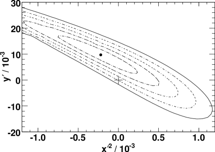
Figure 3: Two-dimensional $1\sigma$-$5\sigma$ contours for $(x^{\prime 2},y^{\prime})$, from BABAR’s fit to the decay time distribution of $D^{0}\!\rightarrow\!K^{+}\pi^{-}$ decays babar_kpi . The contours are calculated from the change in the value of $-2\ln{\cal L}$ from the minimum value, and systematic uncertainties are included. The point is the best-fit value.

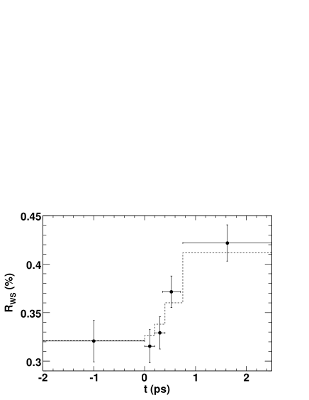
Figure 4: The WS $D^{0}\!\rightarrow\!K^{+}\pi^{-}$ branching fraction for separate bins of decay time, from BABAR babar_kpi . The dashed line shows the expectation based on the values of $(x^{\prime 2},y^{\prime})$ obtained from the decay time fit. The data agrees well with the dashed line but not with a flat (i.e., no mixing) line.

The Belle measurement has somewhat greater statistical precision than that of BABAR, but the central values are in the physical region ($x^{\prime 2}>0$). Belle obtains confidence regions for $x^{\prime 2}$ and $y^{\prime}$ using a toy-MC frequentist method. Due to the proximity of the unphysical region, the procedure uses Feldman-Cousins likelihood ratio ordering FeldmanCousins . The resulting contours are shown in Fig. 5. The CL of the no-mixing point $(0,0)$ is 3.9%, corresponding to $2.1\sigma$. The largest systematic uncertainty arises from variation of the $p_{D^{*}}$ minimum value cut.

Belle searches for $CPV$ by fitting the $D^{0}$ and $\overline{D}{}^{\,0}$ distributions separately. The results, denoted $(x^{\prime 2+},y^{\prime+},R_{D})$ and $(x^{\prime 2-},y^{\prime-},\overline{R}_{D})$, respectively, are used to calculate the $CPV$ parameter $A_{M}=(R^{+}_{M}-R^{-}_{M})/(R^{+}_{M}+R^{-}_{M})$, where $R^{\pm}_{M}=(x^{\prime\pm 2}+y^{\prime\pm 2})/2$. Theoretically, $A_{M}=(|q/p|^{4}-1)/(|q/p|^{4}+1)\approx|q/p|^{2}-1$. The $CPV$ parameter ${\rm Arg}(q/p)\equiv\phi$ and mixing parameters $x^{\prime 2},\,y^{\prime}$ are determined via the relations

$$x^{\prime\pm} = [(1\pm A_{M})/(1\mp A_{M})]^{1/4}(x^{\prime}\cos\phi\pm y^{\prime}\sin\phi)$$

$$y^{\prime\pm} = [(1\pm A_{M})/(1\mp A_{M})]^{1/4}(y^{\prime}\cos\phi\mp x^{\prime}\sin\phi)\,.$$

The resulting confidence region for $(x^{\prime 2},y^{\prime})$ is plotted in Fig. 5 as the solid contour; the complicated shape is due to there being two solutions for $(x^{\prime},y^{\prime})$, depending on the relative sign of $x^{\prime+}$ and $x^{\prime-}$ (which is unmeasured). The fit results are $\phi=(9.4\,\pm 25.3)^{\circ}$ or $(84.5\,\pm 25.3)^{\circ}$ for the same or opposite signs of $x^{\prime+}$ and $x^{\prime-}$, and $A_{M}=0.67\,\pm 1.20$.

Figure 5: 95% C.L. contours for $(x^{\prime 2},y^{\prime})$ from Belle’s analysis of $D^{0}\!\rightarrow\!K^{+}\pi^{-}$ decays belle_kpi : dotted (dashed) is statistical (statistical plus systematic) contour for no $CPV$; solid is statistical plus systematic contour allowing for $CPV$. The point is the best-fit value for no $CPV$. The contours are obtained from a frequentist toy-MC calculation.

IV Dalitz Plot Analysis of $D^{0}\!\rightarrow\!K^{0}_{S}\,\pi^{+}\pi^{-}$

The time dependence of the Dalitz plot for $D^{0}\!\rightarrow\!K^{0}_{S}\,\pi^{+}\pi^{-}$ decays is sensitive to mixing parameters $x$ and $y$ without ambiguity due to strong phases. For a particular point in the Dalitz plot $(m^{2}_{+},m^{2}_{-})$, where $m_{+}\equiv m(K^{0}_{S}\,\pi^{+})$ and $m_{-}\equiv m(K^{0}_{S}\,\pi^{-})$, the overall decay amplitude is

$${\cal A}_{D^{0}}(m^{2}_{+},m^{2}_{-})\,\frac{e_{1}(t)+e_{2}(t)}{2} +$$ (5)

$$\hskip-86.72377pt\left(\frac{q}{p}\right){\cal A}_{\overline{D}{}^{\,0}}(m^{2}_{+},m^{2}_{-})\,\frac{e_{1}(t)-e_{2}(t)}{2}\,,$$

where $e_{(1,2)}(t)=e^{-(im_{1,2}+\Gamma_{1,2}/2)t}$. The first term represents the (time-dependent) amplitude for $D^{0}\!\rightarrow\!K^{0}_{S}\,\pi^{+}\pi^{-}$, and the second term represents the amplitude for $D^{0}\!\!\rightarrow\!\!\overline{D}{}^{\,0}\!\!\rightarrow\!\!K^{0}_{S}\,\pi^{+}\pi^{-}$. Taking the modulus squared of Eq. (5) gives the decay rate or, equivalently, the density of points $\rho(m^{2}_{+},m^{2}_{-};t)$. The result contains terms proportional to $\cosh(y\,\Gamma t)$, $\cos(x\,\Gamma t)$, and $\sin(x\,\Gamma t)$, and thus fitting the time-dependence of $\rho(m^{2}_{+},m^{2}_{-};t)$ determines $x$ and $y$. This method was developed by CLEO cleo_kspp .

To use Eq. (5) requires choosing a model for the decay amplitudes ${\cal A}_{D^{0},\overline{D}{}^{\,0}}(m^{2}_{+},m^{2}_{-})$. This is usually taken to be the “isobar model” isobar , and thus, in addition to $x$ and $y$, one also fits for the magnitudes and phases of various intermediate states. Specifically, ${\cal A}_{D^{0}}(m^{2}_{+},m^{2}_{-})=\sum_{j}a_{j}\,e^{i\delta_{j}}\,A_{j}$, where $\delta_{j}$ is a strong phase, $A_{j}$ is the product of a relativistic Breit-Wigner function and Blatt-Weiskopf form factors, and the parameter $j$ runs over all intermediate states. This sum includes possible scalar resonances and, typically, a constant non-resonant term. For no direct $CPV$, ${\cal A}_{\overline{D}{}^{\,0}}(m^{2}_{+},m^{2}_{-})={\cal A}_{D^{0}}(m^{2}_{-},m^{2}_{+})$; otherwise, one must consider separate decay parameters $(a_{j},\delta_{j})$ for $D^{0}$ decays and $(\bar{a}_{j},\bar{\delta}_{j})$ for $\overline{D}{}^{\,0}$ decays.

Belle has recently fit a large $D^{0}\!\rightarrow\!K^{0}_{S}\,\pi^{+}\pi^{-}$ sample selected from 540 fb^-1 of data belle_kspp . The analysis proceeds in two steps. First, signal and background yields are determined from a two-dimensional fit to variables $M(K\pi\pi)$ and $\Delta M=M(\pi_{s}K\pi\pi)-M(K\pi\pi)$. Within a signal region $|M(K\pi\pi)-M_{D^{0}}|\!<\!15$ MeV/$c^{2}$ and $|\Delta M-5.9{\rm\ MeV}|\!<\!1.0$ MeV (corresponding to $3\sigma$ in resolution), there are 534 000 signal candidates with 95% purity. These events are fit for $x$ and $y$; the (unbinned ML) fit variables are $m^{2}_{+}$, $m^{2}_{-}$, and the decay time $t$. Most of the background is combinatoric, i.e., the $D^{0}$ candidate results from a random combination of tracks. The decay-time distribution of this background is modeled as the sum of a delta function and an exponential function convolved with a Gaussian resolution function, and all parameters are determined from fitting events in the sideband $30{\rm\ MeV}/c^{2}<|M(K\pi\pi)-M_{D^{0}}|<55$ MeV/$c^{2}$.

The results from two separate fits are listed in Table 2. In the first fit $CP$ conservation is assumed, i.e., $q/p\!=\!1$ and ${\cal A}_{\overline{D}{}^{\,0}}(m^{2}_{+},m^{2}_{-})={\cal A}_{D^{0}}(m^{2}_{-},m^{2}_{+})$. The free parameters are $x,y,\tau_{D^{0}}$, some timing resolution function parameters, and decay model parameters $(a_{r},\delta_{r})$. The results for the latter are listed in Table 3. The results for $x$ and $y$ indicate that $x$ is positive, about $2\sigma$ from zero. Projections of the fit are shown in Fig. 6. The fit also yields $\tau_{D}=(409.9\pm 0.9)$ fs, which is consistent with the PDG value pdg (and actually has greater statistical precision).

For the second fit, $CPV$ is allowed and the $D^{0}$ and $\overline{D}{}^{\,0}$ samples are considered separately. This introduces additional parameters $|q/p|$, ${\rm Arg}(q/p)=\phi$, and $(\bar{a}_{j},\bar{\delta}_{j})$. The fit gives two equivalent solutions, $(x,y,\phi)$ and $(-x,-y,\phi+\pi)$. Aside from this possible sign change, the effect upon $x$ and $y$ is small, and the results for $|q/p|$ and $\phi$ are consistent with no $CPV$. The sets of Dalitz parameters $(a_{r},\delta_{r})$ and $(\bar{a}_{r},\bar{\delta}_{r})$ are consistent with each other, indicating no direct $CPV$. Taking $a_{j}\!=\!\bar{a}_{j}$ and $\delta_{j}\!=\!\bar{\delta}_{j}$ (i.e., no direct $CPV$) and repeating the fit gives $|q/p|=0.95\,^{+0.22}_{-0.20}$ and $\phi=(-2\,^{+10}_{-11})^{\circ}$.

The dominant systematic errors are from the time dependence of the Dalitz plot background, and the effect of the $p_{D^{*}}$ momentum cut used to reject $D^{*}$’s originating from $B$ decays. The default fit includes $\pi\pi$ scalar resonances $\sigma_{1}$ and $\sigma_{2}$; when evaluating systematic errors, the fit is repeated without any $\pi\pi$ scalar resonances using $K$-matrix formalism K-matrix . The influence upon $x$ and $y$ is small and included as a systematic error.

The 95% C.L. contour for $(x,y)$ is plotted in Fig. 7. The contour is obtained from the locus of points where $-2\ln{\cal L}$ rises by 5.99 units from the minimum value; the distance of the points from the origin is subsequently rescaled to include systematic uncertainty. We note that for the $CPV$-allowed case, the reflections of the contours through the origin are also allowed regions.

Table 2: Fit results and 95% C.L. intervals for $x$ and $y$, from Belle’s analysis of $D^{0}\!\rightarrow\!K^{0}_{S}\,\pi^{+}\pi^{-}$ decays belle_kspp . The errors are statistical, experimental systematic, and decay-model systematic, respectively.

Fit	Param.	Result	95% C.L. inter.
No	$x\,(\%)$	$0.80\,\pm 0.29\,^{+0.09\,+0.10}_{-0.07\,-0.14}$	$(0.0,1.6)$
$CPV$	$y\,(\%)$	$0.33\,\pm 0.24\,^{+0.08\,+0.06}_{-0.12\,-0.08}$	$(-0.34,0.96)$
$CPV$	$x\,(\%)$	$0.81\,\pm 0.30\,^{+0.10\,+0.09}_{-0.07\,-0.16}$	$|x|<1.6$
	$y\,(\%)$	$0.37\,\pm 0.25\,^{+0.07\,+0.07}_{-0.13\,-0.08}$	$|y|<1.04$
	$|q/p|$	$0.86\,^{+0.30\,+0.06}_{-0.29\,-0.03}\,\pm 0.08$	$-$
	$\phi\,(^{\circ})$	$-14\,^{+16\,+5\,+2}_{-18\,-3\,-4}$	$-$

Table 3: Fit results for $D^{0}\!\rightarrow\!K^{0}_{S}\,\pi^{+}\pi^{-}$ Dalitz plot parameters, from Belle belle_kspp . The errors are statistical only. The fit fraction is defined as the ratio of the integral $\int|a_{r}\,{\cal A}_{r}(m^{2}_{-}\,,m^{2}_{+})|^{2}\,dm^{2}_{-}\,dm^{2}_{+}$ to $\int|\sum_{r=1}^{n}a_{r}\,e^{i\phi_{r}}{\cal A}_{r}(m^{2}_{-}\,,m^{2}_{+})|^{2}\,dm^{2}_{-}\,dm^{2}_{+}$.

Resonance	Amplitude	Phase (deg)	Fit fraction
$K^{*}(892)^{-}$	$1.629\pm 0.006$	$134.3\pm 0.3$	0.6227
$K_{0}^{*}(1430)^{-}$	$2.12\pm 0.02$	$-0.9\pm 0.8$	0.0724
$K_{2}^{*}(1430)^{-}$	$0.87\pm 0.02$	$-47.3\pm 1.2$	0.0133
$K^{*}(1410)^{-}$	$0.65\pm 0.03$	$111\pm 4$	0.0048
$K^{*}(1680)^{-}$	$0.60\pm 0.25$	$147\pm 29$	0.0002
$K^{*}(892)^{+}$	$0.152\pm 0.003$	$-37.5\pm 1.3$	0.0054
$K_{0}^{*}(1430)^{+}$	$0.541\pm 0.019$	$91.8\pm 2.1$	0.0047
$K_{2}^{*}(1430)^{+}$	$0.276\pm 0.013$	$-106\pm 3$	0.0013
$K^{*}(1410)^{+}$	$0.33\pm 0.02$	$-102\pm 4$	0.0013
$K^{*}(1680)^{+}$	$0.73\pm 0.16$	$103\pm 11$	0.0004
$\rho(770)$	1 (fixed)	0 (fixed)	0.2111
$\omega(782)$	$0.0380\pm 0.0007$	$115.1\pm 1.1$	0.0063
$f_{0}(980)$	$0.380\pm 0.004$	$-147.1\pm 1.1$	0.0452
$f_{0}(1370)$	$1.46\pm 0.05$	$98.6\pm 1.8$	0.0162
$f_{2}(1270)$	$1.43\pm 0.02$	$-13.6\pm 1.2$	0.0180
$\rho(1450)$	$0.72\pm 0.04$	$41\pm 7$	0.0024
$\sigma_{1}$	$1.39\pm 0.02$	$-146.6\pm 0.9$	0.0914
$\sigma_{2}$	$0.267\pm 0.013$	$-157\pm 3$	0.0088
NR	$2.36\pm 0.07$	$155\pm 2$	0.0615

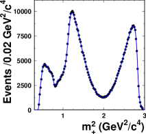
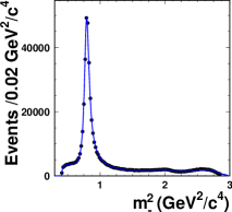
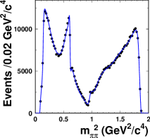
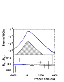
Figure 6: Projection of the unbinned ML fit superimposed on the data for $D^{0}\!\rightarrow\!K^{0}_{S}\,\pi^{+}\pi^{-}$ decays, from Belle belle_kspp . In (d), the hatched area represents the combinatorial background contribution, and the lower plot shows the ratio of decay-time distributions for events in the $K^{*}(892)^{+}$ and $K^{*}(892)^{-}$ regions, where sensitivity to $(x,y)$ is highest.

Figure 7: 95% C.L. contours for $(x,y)$ from Belle belle_kspp : dotted (solid) is statistical (statistical plus systematic) contour for no $CPV$; dashed-dotted (dashed) is statistical (statistical plus systematic) contour allowing for $CPV$. The point is the best-fit value for no $CPV$.

V Combining all Measurements

All mixing measurements can be combined to obtain world average (WA) values for $x$ and $y$. The Heavy Flavor Averaging Group (HFAG) has done such a combination by adding together log-likelihood functions obtained from analyses of $D^{0}\!\rightarrow\!K^{+}\ell\nu$, $D^{0}\!\rightarrow\!h^{+}h^{-}$, $D^{0}\!\rightarrow\!K^{+}\pi^{-}$, $D^{0}\!\rightarrow\!K^{+}\pi^{-}\pi^{0}$, $D^{0}\!\rightarrow\!K^{+}\pi^{-}\pi^{+}\pi^{-}$, and $D^{0}\!\rightarrow\!K^{0}_{S}\,\pi^{+}\pi^{-}$ decays, as well as CLEOc results for double-tagged branching fractions measured at the $\psi(3770)$ resonance hfag_charm . The combination of likelihood functions preserves correlations among parameters and also accounts for non-Gaussian errors. When using this method, HFAG assumes negligible $CPV$.

As a first step, WA values for $y_{\rm CP}$ and $R_{M}$ are calculated by taking weighted averages of independent experimental measurements – see Figs. 8 and 9.These results are then converted to three-dimensional likelihood functions for $(x,y,\delta)$. For example, the measurement of $y_{CP}$ gives a parabolic log-likelihood function in $y$ and flat distributions in $x$ and $\delta$. The $R_{M}$ likelihood function is an annulus in the $x$-$y$ plane and a flat distribution in $\delta$.

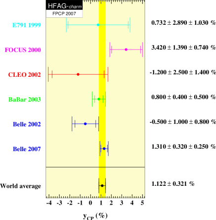
Figure 8: World average value for $y_{\rm CP}$, from HFAG hfag_charm .

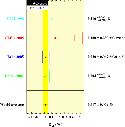
Figure 9: World average value for $R_{M}$, from HFAG hfag_charm .

The logarithm of the likelihood functions are added, and the result is added to the $(x,y,\delta)$ log-likelihood function obtained from $D^{0}\!\rightarrow\!K^{+}\pi^{-}$ decays. The latter is determined as follows. The experiments directly measure a likelihood function ${\cal L}(x^{\prime 2},y^{\prime},R_{D})$; thus one first projects out $R_{D}$ by allowing it to take, for any $(x^{\prime 2},y^{\prime})$ point, its preferred value. The resulting likelihood for $(x^{\prime 2},y^{\prime})$ is converted to ${\cal L}(x,y,\delta)$ by scanning values of $(x,y,\delta)$, calculating the corresponding values of $(x^{\prime 2},y^{\prime})$, and assigning the likelihood for that $(x^{\prime 2},y^{\prime})$ bin. This method ignores unphysical (negative) values of $x^{\prime 2}$. The resulting function ${\cal L}(x,y,\delta)$ is added to those obtained from $y_{\rm CP}$, $R_{M}$, and other measurements. The final likelihood function is projected onto the $(x,y)$ plane by letting $\delta$ take, for any $(x,y)$ point, its preferred value. This projection is shown in Fig. 10. The unusual shape around $x\!=\!y\!=\!0$ is mainly due to $D^{0}\!\rightarrow\!K^{+}\pi^{-}$ decays, which disfavor the no-mixing point. At $x\!=\!y\!=\!0$, $-2\ln{\cal L}$ rises by 37 units above the minimum value; this difference implies that the no-mixing point is excluded at the level of $5.7\sigma$.

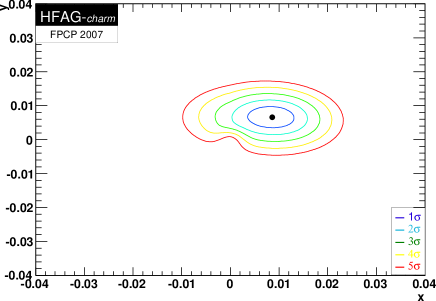
Figure 10: Two-dimensional $1\sigma$-$5\sigma$ contours for $(x,y)$, obtained by adding log-likelihoods from measurements of $D^{0}\!\rightarrow\!K^{+}\ell\nu$, $D^{0}\!\rightarrow\!h^{+}h^{-}$, $D^{0}\!\rightarrow\!K^{+}\pi^{-}$, $D^{0}\!\rightarrow\!K^{+}\pi^{-}\pi^{0}$, $D^{0}\!\rightarrow\!K^{+}\pi^{-}\pi^{+}\pi^{-}$, and $D^{0}\!\rightarrow\!K^{0}_{S}\,\pi^{+}\pi^{-}$ decays, and double-tagged branching fractions measured at the $\psi(3770)$ resonance (from HFAG hfag_charm ).

The likelihood function is condensed to one dimension by letting, for any value of $x$ $(y)$, the parameter $y$ $(x)$ take its preferred value. The resulting likelihoods for $(x,y)$ give central values and 68.3% C.L. intervals

$$x = (0.87\,^{+0.30}_{-0.34})\%$$ (6)

$$y = (0.66\,^{+0.21}_{-0.20})\%\,.$$ (7)

The former is $2.6\sigma$ from zero, and the latter is $3.2\sigma$ from zero.

In summary, we conclude the following:

• the experimental data consistently indicates that $D^{0}$’s undergo mixing. The effect is presumably dominated by long-distance processes, and unless $|x|\gg|y|$, it may be difficult to identify new physics from mixing alone.

• Since $y_{\rm CP}$ is positive, the $CP$-even state is shorter-lived, as in the $K^{0}$-$\overline{K}{}^{\,0}$ system. However, since $x$ appears to be positive, the $CP$-even state is heavier, unlike in the $K^{0}$-$\overline{K}{}^{\,0}$ system.

• There is no evidence yet for $CPV$ in the $D^{0}$-$\overline{D}{}^{\,0}$ system.

- (1) M. Staric et al. (Belle), Phys. Rev. Lett. 98, 211803 (2007).
- (2) B. Aubert et al. (BABAR), Phys. Rev. Lett. 98, 211802 (2007).
- (3) Charge-conjugate modes are included unless noted otherwise.
- (4) A. A. Petrov, eConf C030603, MEC05 (2003) arXiv:hep-ph/0311371.
- (5) U. Bitenc et al. (Belle), Phys. Rev. D 72, 071101 (2005).
- (6) G. Feldman and R. Cousins, Phys. Rev. D 57, 3873 (1998).
- (7) B. Aubert et al. (BABAR), arXiv:0705.0704 (2007).
- (8) Y. Nir, arXiv:hep-ph/0703235 (2007).
- (9) E. M. Aitala et al. (E791), Phys. Rev. Lett. 83, 32 (1999); J. M. Link et al. (FOCUS), Phys. Lett. B 485, 62 (2000); S. E. Csorna et al. (CLEO), Phys. Rev. D 65, 092001 (2002); B. Aubert et al. (BABAR), Phys. Rev. Lett. 91, 121801 (2003).
- (10) W.-M. Yao et al. (PDG), Jour. of Phys. G 33, 1 (2006).
- (11) L. M. Zhang et al. (Belle), Phys. Rev. Lett. 96, 151801 (2006).
- (12) D. M. Asner et al. (CLEO), Phys. Rev. D 72, 012001 (2005); arXiv:hep-ex/0503045 (revised April, 2007).
- (13) A. Poluektov et al. (Belle), Phys. Rev. D 73, 112009 (2006); S. Kopp et al. (CLEO), Phys. Rev. D 63, 092001 (2001).
- (14) L. M. Zhang et al. (Belle), arXiv:0704.1000 (2007).
- (15) J. M. Link et al. (FOCUS), Phys. Lett. B 585, 200 (2004); B. Aubert et al. (BABAR), arXiv:hep-ex/0507101 (2005).
- (16) http://www.slac.stanford.edu/xorg/hfag/charm/index.html