Thermodynamic modeling of the Hf-Si-O system

Abstract

The Hf-O system has been modeled by combining existing experimental data and first-principles calculations results through the CALPHAD approach. Special quasirandom structures of $\alpha$ and $\beta$ hafnium were generated to calculate the mixing behavior of oxygen and vacancies. For the total energy of oxygen, vibrational, rotational and translational degrees of freedom were considered. The Hf-O system was combined with previously modeled Hf-Si and Si-O systems, and the ternary compound in the Hf-Si-O system, HfSiO₄ has been introduced to calculate the stability diagrams pertinent to the thin film processing.

1 Introduction

The Hf-O system has been considered as one of the most important systems in various industrial fields, such as nuclear materials and high temperature/pressure materials. Hafnium dioxide is known as the least volatile of all the oxides and its high melting point, extreme chemical inertness, and high thermal neutron capture cross section make it suitable for use as control rods or neutron shielding. All of these reasons can make HfO₂ a promising refractory material for future nuclear applications[1].

Recently, the Hf-O system has even attracted considerable attention for semi-conductor materials. The current gate oxide material (SiO₂ in general) thickness in advanced complementary metal-oxide semiconductor (CMOS) integrated circuits has continuously decreased and has reached the current process limit[2]. One solution to further improve their performance is to use alternative materials with higher dielectric constants (k), such as ZrO₂ and HfO₂[3, 4]. In this regard, thermodynamic stability calculations results showed that the interface between HfO₂ and Si is found to be stable with respect to the formation of silicides whereas the ZrO₂/Si interface is not[5]. The stability of the HfO₂/Si interface make the use of this oxide even more promising.

The other important group IVA transition metals, such as Ti and Zr, which show very similar behavior as Hf, with oxygen are modeled recently by Waldner and Eriksson [6] and Wang et al. [7] respectively. All these systems commonly have a wide oxygen solubility ranges in the hcp phase, up to 33 at.%(Ti-O), 29 at.%(Zr-O), and 20 at.%(Hf-O) at room temperature, as derived from higher temperature measurements.

In the present work, the Hf-O system has been modeled with the existing experimental data and first-principles calculations results. Afterwards, combining with the thermodynamic parameters of the Hf-Si and the Si-O binary systems, the thermodynamic description of the Hf-Si-O ternary system is obtained, and the stability diagrams pertinent to thin film processing, such as the HfO₂-SiO₂ pseudo-binary, the isopleth of HfO₂-Si, and isothermal sections are calculated.

2 Experimental data

2.1 Phase diagram data

2.1.1 Hf-O

Many investigations have been conducted to clarify the phase diagram of the Hf-O system[8, 9, 10, 11]. The main issues regarding the phase diagram of the Hf-O system include: the extent of the $\alpha$-Hf solid solution, the congruent melting of HfO₂, and the allotropic transformations of HfO₂.

The phase diagrams suggested by Rudy and Stecher [8] and Domagala and Ruh [9] are quite similar to each other, except the formation of the $\beta$-Hf phase and the eutectic reaction around 37 at.% oxygen of liquid. For the hafnium rich-side, Rudy and Stecher [8] proposed a eutectic reaction at 2273K, while Domagala and Ruh [9] suggested a peritectic reaction around 2523K. Similar to other group IVA transition metals, such as Ti, and Zr, it is strongly believed that Hf also has a peritectic reaction at the Hf-rich side. Another minor disagreement between these two phase diagram determinations is the eutectic reaction, Liquid $\rightarrow$ $\alpha$ + HfO₂. Rudy and Stecher suggested composition of oxygen in the liquid as 40 at.% O and 2453$\pm$40K, while Domgala and Ruh proposed 37 at.% O and $\sim$2473K.

For the $\alpha$-Hf solid solution, these two works[8, 9] are in quite good agreement with each other. Rudy and Stecher found that $\alpha$-Hf dissolves up to 20.5 at.% oxygen at 1623K and that the solubility range is almost independent of temperature; this shows consistency with observations by Domagala and Ruh and they quoted a solubility of oxygen in $\alpha$-Hf of 18.6 at.% at 1273K.

Ruh and Patel [11] proposed a tentative phase diagram for the $\rm HfO_{2}$-rich portion of the Hf-HfO₂ system on the basis of metallographic data. They suggested the existence of solid solution regions for both cubic and tetragonal phases deviated from the stoichiometric composition of HfO₂. Since the important phases in the Hf-O system are the polymorphs of the $\rm HfO_{2}$ phases, i.e. monoclinic, tetragonal, and cubic, they have been studied extensively[12, 13, 14, 15, 16]. Allotropic transformations of the HfO₂ phase have been well summarized by Wang et al. [17].

The suggested phase diagram of the Hf-O system by Massalski [18] is shown in Fig. 1 .

Figure 1: Proposed phase diagram of the Hf-O system from Massalski [18].

2.1.2 Hf-Si-O

Not many studies have been conducted regarding the phase stabilities of the Hf-Si-O ternary system. Speer and Cooper [19] reported a ternary compound, Hafnon, with the chemical formula of HfSiO₄ and the crystal structure as $I4_{1}/amd$. One of the most important phase diagrams of the Hf-Si-O system is the HfO₂-SiO₂ pseudo-binary that includes HfSiO₄ since the phase stabilities of this pseudo-binary are pertinent to the processing of the dielectric thin film. Parfenenkov et al. [20] determined the melting of HfSiO₄ at 2023$\pm$15K.

2.2 Thermochemical data

As discussed in the introduction, the Hf-O system has a wide range of oxygen solubility in the hcp phase. Hirabayashi et al. studied order/disorder transformation of interstitial oxygen in hafnium[21] around 10 $\sim$ 20at.% by electron microscopy and neutron and X-ray diffractions. This work revealed that two types of interstitial superstructures are formed in the hypo- and hyper-stoichiometric compositions near $\rm HfO_{1/6}$ below 700K which have $R\bar{3}$ and $P\bar{3}1c$ symmetries, respectively.

For the completely disordered hcp phase at high temperature, Boureau and Gerdanian [22] measured the partial molar enthalpy of solution of oxygen in $\alpha$-Hf solid solution at 1323K as a function of oxygen content using a Tian-Calvet-type microcalorimeter. Previously, it was almost impossible to measure the extremely low oxygen pressure in equilibrium with hafnium-oxygen solutions. Therefore derivation from the second law of thermodynamics was the only way to acquire thermodynamic information of solid solution phases[23, 24]. The major difficulty of direct measurement is making sure that all the hafnium surface is accessible at the same time to oxygen. Boureau and Gerdanian improved the accuracy of measurement by solving the geometrical effect of specimen and oxygen contact. The observed phase boundary of $\alpha$-Hf in this work is consistent with that of previous phase diagram studies[8, 9] as O/Hf=0.255.

3 First-principles calculations

3.1 Methodology

The Vienna Ab initio Simulation Package (VASP)[25] was used to perform the Density Functional Theory (DFT) electronic structure calculations. The projector augmented wave (PAW) method[26] was chosen and the general gradient approximation (GGA)[27] was used to take into account exchange and correlation contributions to the hamiltonian of the ion-electron system. An energy cutoff of 500 eV was used to calculate the electronic structures of all the compounds. 5,000 k-points per reciprocal atom based on the Monkhorst-Pack scheme for the Brillouin-zone sampling was used. The $k$-point meshes were centered at the $\Gamma$ point for the hcp calculations.

3.2 Ordered phases

The ordered structures of the Hf-Si-O system calculated in this work can be categorized into three groups. First, pure elements, i.e. hcp hafnium and diamond silicon are calculated for the reference states. Second, hypothetical compounds, the end-members of the $\alpha$, $\beta$ solid solutions (HfO_0.5 and HfO₃), are also calculated. The stable compounds, monoclinic HfO₂, quartz SiO₂, and the ternary compounds, HfSiO₄ are calculated as well. The calculated results of the ordered structures are listed in Table 1. The enthalpy of those compounds are calculated from Eqn. 3.2:

$$\Delta H^{Hf_{x}Si_{y}O_{z}}_{f}= H(Hf_{x}Si_{y}O_{z})-\tfrac{x}{x+y+z}H(Hf)$$

$$-\tfrac{y}{x+y+z}H(Si)-\tfrac{z}{x+y+z}H(O)$$ (1)

where $H$ corresponds to the enthalpies of the compound and reference structures. The reference states for Hf and Si were the hcp and diamond structures, respectively. In the case of condensed phases, the effects of lattice vibrations and other degrees of freedom (i.e. electronic, magnetic) can be neglected at low temperatures. Moreover, due to their rather small molar volumes, the $PV$ contributions to their enthalpies ($H\equiv U+PV$) can also be neglected. Thus their enthalpies $H$, can be replaced by the calculated first-principles total energies at 0K in Eqn. 3.2. For the oxygen gas, the selected reference state was diatomic oxygen, O₂. In this case, the contributions due to vibrational and translational degrees of freedom, as well as the $PV$ work term, the molar volume of O₂ is much larger than that of the condensed phases and cannot be neglected. In the following section, the determination of the correct reference state for O₂ will be briefly discussed.

Table 1: First-principles calculation results of pure elements, hypothetical compounds ($\alpha$, $\beta$-Hf), and stable compounds (HfO₂, SiO₂, and HfSiO₄). By definition, $\Delta H^{f}$ of pure elements are zero. Reference states for all the compounds are SER.

Phases	Space	Lattice parameters (Å)			Total energy	$\Delta H^{f}$
	Group	a	b	c	(eV/atom)	(kJ/mol-atom)
HCP_A3 (Hf)	$P6_{3}/mmc$	3.198	3.198	5.053	-9.8320	0
Diamond_A4 (Si)	$Fd\bar{3}m$	5.468	5.468	5.468	-5.4315	0
Gas (O2)					-4.7936	0
$\alpha$-Hf (HfO0.5)	$P\bar{3}m1$	3.225	3.225	5.150	-9.9718	-175.511
$\beta$-Hf (HfO3)	$Im\bar{3}m$	4.364	4.364	4.364	-7.7253	-161.308
Monoclinic(HfO2)a	$P2_{1}/c$	5.135	5.194	5.314	-10.2101	-360.563
Quartz (SiO2)	$P3_{2}21$	5.007	5.007	5.496	-7.9581	-284.809
HfSiO4	$I4_{1}/amd$	6.616	6.616	6.004	-9.1024	-324.453
						-1.769b

• ^a $\beta$=99.56^∘

• ^b Reference states are monoclinic (HfO₂) and quartz (SiO₂).

3.3 Oxygen calculation

The selected reference state for oxygen corresponds to the diatomic molecule at 298K. Two oxygen atoms were placed in a ’big box’ to model the oxygen molecule gas and completely relaxed to find the lowest energy configuration. In order to properly account for the net magnetic moment of this molecule, spin polarization was considered. It was necessary to take into account the contributions of vibrational, rotational and translational degrees of freedom at finite temperature. Under the harmonic oscillator-rigid rotor approximation at temperatures greater than the characteristic rotational temperature— 2.07K for O₂—the internal energy of the O₂ molecule is given by [28]:

$$E(T)=k_{B}T\left(\frac{5}{2}+\frac{\Theta_{\nu}}{2}+\frac{\Theta_{\nu}/T}{e^{\Theta_{\nu}/T}-1}\right)+E_{0}$$ (2)

where $\Theta_{\nu}$ is the characteristic vibrational temperature. The first term in Eqn. 2 corresponds to the contributions due to translational and rotational degrees of freedom and the second and third terms correspond to vibrational contributions. The last term, E₀, corresponds to the energy of the ground electronic state at 0K. By including the $PV=k_{B}T$ term of an ideal, non-interacting gas in Eqn. 2, the enthalpy of the diatomic O₂ molecule can be obtained. The difference between the ground state electronic energy and the enthalpy of O₂, per atom, is given by:

$$H(T)^{O_{2}}-E_{0}^{O_{2}}=\frac{k_{B}T}{2}\left(\frac{7}{2}+\frac{\Theta_{\nu}}{2}+\frac{\Theta_{\nu}/T}{e^{\Theta_{\nu}/T}-1}\right)$$ (3)

In the case of O₂, the characteristic vibrational temperature, $\Theta_{\nu}$ is 2256K [28]. At 298K, the value of $H(T)^{O_{2}}-E_{0}^{O_{2}}$ is +0.0936 eV/atom or +9.03 kJ/mol-atom.

3.4 Disordered phases: Special quasirandom structures

In order to calculate the enthalpies of mixing of oxygen and vacancy for both hcp and bcc phases in the Hf-O system, special quasirandom structures (SQS)[29] are used which are supercells with correlation functions as close as possible to those of a completely random solution phase.

In order to introduce the special quasirandom structure, it is convenient to understand the concept of correlation functions. In any atomic arrangements, the geometrical correlation between atoms in the structure can be defined as to whether it is ordered or disordered. For a completely disordered structure, the surrounding environment of an atom at any given sites should be the same as all the other lattice sites. Correlation functions, $\prod_{k,m}$, are defined as the products of site occupation numbers of different figures, $k$, such as point, pair, triplet (when $k=1,2,3,\dots$) and so forth. The correlation functions of each figure can be grouped together based on the distance from a lattice site as m^th nearest-neighbors.

For a binary system, a spin variable, $\sigma=\pm 1$, can be assigned to different types of atomic occupations and their products represent the correlation functions of binary alloys. The correlation function of a random alloy is simply described as $(2x-1)^{k}$ in the $A_{1-x}B_{x}$ substitutional binary alloy, where $x$ is the composition. Once such a supercell satisfies the correlation function of a target structure, it can be easily transferred to other systems by simply switching the types of atoms in the structure.

The major drawback of SQS is that the concentration which can be calculated is typically limited to 25, 50, and 75 at.% since the correlation functions for completely random structures other than those three compositions are almost impossible to satisfy with a small number of atoms. In principle, one can find a bigger supercell which has better correlation functions than smaller ones; however, such a calculation requires expensive computing. On the other hand, three data points from SQS calculations can clearly indicate the mixing behavior of solution phases. Another disadvantage of SQS is that it cannot consider the long range interaction since the size of the structure itself is limited. It is reported that SQS works well with a system where short range interactions are dominant[30, 31].

Three different compositions, i.e. $y_{O}$ = 0.25, 0.5, and 0.75 with $y_{O}$ representing the mole fraction of oxygen in the hcp and bcc interstitial sites, were considered and only two structures were generated in both phases since the structures of $y_{O}=0.25$ and 0.75 are switchable to each other. For the $\alpha$ solid solution,the total number of lattice sites considered were 24, 36, and 48. Since only the mixing between oxygen and vacancies are considered to generate a SQS for the hcp and bcc phases, the hafnium ions are excluded from the correlation function calculations. Therefore, the total number of oxygen and vacancies are 8, 12, and 16, respectively. For the $\beta$ solid solution, the total number of lattice sites that were considered for the mixing of oxygen and vacancy were 12 and 24 with total number of sites being 16 and 32, respectively. The complete descriptions of the SQS’s for $\alpha$ and $\beta$ solid solutions are listed in Tables 2 and 3, and their correlation functions are given in Tables 4 and 5. Finding bigger cells than these were prohibited by the limited computing resources.

Table 2: Structural descriptions of the SQS-$N$ structures for the $\alpha$ solid solution. Lattice vectors and atom/vacancy positions are given in fractional coordinates of the supercell. Atomic positions are given for the ideal, unrelaxed hcp sites. Translated Hf positions are not listed. Original Hf positions in the primitive cell are (0 0 0) and ($\tfrac{2}{3}$ $\tfrac{1}{3}$ $\tfrac{1}{2}$).

Oxygen %	50			75
SQS-$N$	24	36	48	48
Lattice vectors	$\left(\begin{array}[]{rrr}1&0&-1\\ -1&-2&0\\ -3&0&-1\\ \end{array}\right)$	$\left(\begin{array}[]{rrr}1&-1&1\\ -2&-2&1\\ -1&-3&-1\\ \end{array}\right)$	$\left(\begin{array}[]{rrr}0&-2&0\\ 0&0&-2\\ 4&2&0\\ \end{array}\right)$	$\left(\begin{array}[]{rrr}2&1&-1\\ 0&-2&-1\\ -2&1&-2\\ \end{array}\right)$
O	$\begin{array}[t]{rrr}\tfrac{1}{3}&\tfrac{1}{3}&-\tfrac{3}{4}\\ -1\tfrac{2}{3}&-1\tfrac{1}{3}&-\tfrac{3}{4}\\ -\tfrac{2}{3}&-1\tfrac{1}{3}&-\tfrac{3}{4}\\ -2\tfrac{2}{3}&-1\tfrac{1}{3}&-1\tfrac{3}{4}\\ \end{array}$	$\begin{array}[t]{rrr}-\tfrac{2}{3}&-2\tfrac{1}{3}&\tfrac{1}{4}\\ -1\tfrac{2}{3}&-2\tfrac{1}{3}&1\tfrac{1}{4}\\ -2\tfrac{2}{3}&-4\tfrac{1}{3}&\tfrac{1}{4}\\ -\tfrac{2}{3}&-2\tfrac{1}{3}&1\tfrac{1}{4}\\ -1\tfrac{2}{3}&-4\tfrac{1}{3}&\tfrac{1}{4}\\ -\tfrac{2}{3}&-4\tfrac{1}{3}&\tfrac{1}{4}\\ \end{array}$	$\begin{array}[t]{rrr}\tfrac{1}{3}&-1\tfrac{1}{3}&-\tfrac{3}{4}\\ 2\tfrac{1}{3}&-\tfrac{1}{3}&-\tfrac{3}{4}\\ 3\tfrac{1}{3}&-\tfrac{1}{3}&-\tfrac{3}{4}\\ 1\tfrac{1}{3}&-1\tfrac{1}{3}&-1\tfrac{3}{4}\\ 2\tfrac{1}{3}&\tfrac{2}{3}&-1\tfrac{3}{4}\\ 3\tfrac{1}{3}&\tfrac{2}{3}&-1\tfrac{3}{4}\\ 2\tfrac{1}{3}&-\tfrac{1}{3}&-1\tfrac{3}{4}\\ 3\tfrac{1}{3}&-\tfrac{1}{3}&-1\tfrac{3}{4}\\ \end{array}$	$\begin{array}[t]{rrr}-\tfrac{2}{3}&\tfrac{2}{3}&-2\tfrac{3}{4}\\ \tfrac{1}{3}&\tfrac{2}{3}&-2\tfrac{3}{4}\\ \tfrac{1}{3}&1\tfrac{2}{3}&-2\tfrac{3}{4}\\ -\tfrac{2}{3}&-\tfrac{1}{3}&-1\tfrac{3}{4}\\ 1\tfrac{1}{3}&-\tfrac{1}{3}&-1\tfrac{3}{4}\\ -\tfrac{2}{3}&\tfrac{2}{3}&-1\tfrac{3}{4}\\ \tfrac{1}{3}&\tfrac{2}{3}&-1\tfrac{3}{4}\\ 1\tfrac{1}{3}&\tfrac{2}{3}&-1\tfrac{3}{4}\\ -\tfrac{2}{3}&-\tfrac{1}{3}&-2\tfrac{3}{4}\\ \tfrac{1}{3}&-\tfrac{1}{3}&-2\tfrac{3}{4}\\ -\tfrac{2}{3}&-1\tfrac{1}{3}&-1\tfrac{3}{4}\\ \tfrac{1}{3}&-\tfrac{1}{3}&-\tfrac{3}{4}\\ \end{array}$
Va	$\begin{array}[t]{rrr}-1\tfrac{2}{3}&-\tfrac{1}{3}&-1\tfrac{3}{4}\\ -1\tfrac{2}{3}&-\tfrac{1}{3}&-\tfrac{3}{4}\\ -\tfrac{2}{3}&-\tfrac{1}{3}&-\tfrac{3}{4}\\ -2\tfrac{2}{3}&-1\tfrac{1}{3}&-\tfrac{3}{4}\\ \end{array}$	$\begin{array}[t]{rrr}-1\tfrac{2}{3}&-3\tfrac{1}{3}&\tfrac{1}{4}\\ -\tfrac{2}{3}&-3\tfrac{1}{3}&\tfrac{1}{4}\\ -1\tfrac{2}{3}&-4\tfrac{1}{3}&1\tfrac{1}{4}\\ -\tfrac{2}{3}&-1\tfrac{1}{3}&\tfrac{1}{4}\\ -1\tfrac{2}{3}&-3\tfrac{1}{3}&1\tfrac{1}{4}\\ -\tfrac{2}{3}&-3\tfrac{1}{3}&1\tfrac{1}{4}\\ \end{array}$	$\begin{array}[t]{rrr}\tfrac{1}{3}&-\tfrac{1}{3}&-\tfrac{3}{4}\\ 1\tfrac{1}{3}&-\tfrac{1}{3}&-\tfrac{3}{4}\\ 1\tfrac{1}{3}&-1\tfrac{1}{3}&-\tfrac{3}{4}\\ 2\tfrac{1}{3}&\tfrac{2}{3}&-\tfrac{3}{4}\\ 3\tfrac{1}{3}&\tfrac{2}{3}&-\tfrac{3}{4}\\ \tfrac{1}{3}&-\tfrac{1}{3}&-1\tfrac{3}{4}\\ 1\tfrac{1}{3}&-\tfrac{1}{3}&-1\tfrac{3}{4}\\ \tfrac{1}{3}&-1\tfrac{1}{3}&-1\tfrac{3}{4}\\ \end{array}$	$\begin{array}[t]{rrr}\tfrac{1}{3}&-\tfrac{1}{3}&-1\tfrac{3}{4}\\ \tfrac{1}{3}&-1\tfrac{1}{3}&-1\tfrac{3}{4}\\ 1\tfrac{1}{3}&\tfrac{2}{3}&-\tfrac{3}{4}\\ -1\tfrac{2}{3}&-\tfrac{1}{3}&-2\tfrac{3}{4}\\ \end{array}$

Table 3: Structural descriptions of the SQS-$N$ structures for the $\beta$ solid solution. Lattice vectors and atom/vacancy positions are given in fractional coordinates of the supercell. Atomic positions are given for the ideal, unrelaxed bcc sites. Translated Hf positions are not listed. The original Hf position in the primitive cell is (0 0 0).

Oxygen %	50		75
SQS-$N$	16	32	32
Lattice vectors	$\left(\begin{array}[]{rrr}0.5&0.5&1.5\\ -0.5&1.5&0.5\\ -0.5&-1.5&-0.5\\ \end{array}\right)$	$\left(\begin{array}[]{rrr}-1&0&0\\ 0&1&-1\\ 0&-2&-2\\ \end{array}\right)$	$\left(\begin{array}[]{rrr}0&0&2\\ 0&2&0\\ -1&0&0\\ \end{array}\right)$
O	$\begin{array}[t]{rrr}0&0&0.5\\ -0.5&1&1\\ -0.5&0&1\\ 0&-0.5&1\\ 0&1&1.5\\ 0&0.5&1.5\\ \end{array}$	$\begin{array}[t]{rrr}-1&0&-0.5\\ -1&0.5&-1.5\\ -0.5&0&-1.5\\ -1&0.5&-1\\ -0.5&0.5&-1\\ -1&-1&-1.5\\ -1&-0.5&-2.5\\ -1&-0.5&-1\\ -0.5&0&-2\\ -1&-0.5&-2\\ -0.5&-0.5&-2\\ -0.5&-1&-2\\ \end{array}$	$\begin{array}[t]{rrr}-0.5&2&1.5\\ -0.5&1&1.5\\ -1&1&1.5\\ -1&0.5&1.5\\ 0.5&2&0.5\\ 1&2&0.5\\ -1&1.5&0.5\\ -1&1&0.5\\ -1&0.5&0.5\\ -1&1.5&1\\ -0.5&1.5&1\\ -0.5&1&1\\ -1&0.5&1\\ -0.5&0.5&1\\ -0.5&2&1\\ 0.5&1.5&2\\ -0.5&1&2\\ -1&0.5&2\\ \end{array}$
Va	$\begin{array}[t]{rrr}-0.5&1&0.5\\ -0.5&-0.5&0\\ -0.5&-1&0\\ -0.5&0&0.5\\ 0&0.5&1\\ -0.5&0.5&1\\ \end{array}$	$\begin{array}[t]{rrr}-0.5&-1&-2.5\\ -1&-1&-2.5\\ -1&-1.5&-2.5\\ -0.5&0&-0.5\\ -1&-1.5&-2\\ -0.5&-1.5&-2\\ -0.5&-1&-3\\ -1&0&-1.5\\ -1&-0.5&-1.5\\ -0.5&0&-1\\ -0.5&-1&-1.5\\ -0.5&-0.5&-1\\ \end{array}$	$\begin{array}[t]{rrr}-1&2&1.5\\ -1&1.5&1.5\\ -0.5&1&0.5\\ -1&1.5&2\\ -0.5&0.5&2\\ -0.5&2&2\\ \end{array}$

Table 4: Pair and multi-site correlation functions of SQS-$N$ structures for $\alpha$ solid solution when the c/a ratio is ideal. The number in the square bracket next to $\overline{\Pi}_{k,m}$ is the number of equivalent figures at the same distance in the structure.

Oxygen %	50				75
SQS-$N$	Random	24	36	48	Random	48
$\overline{\Pi}_{2,1}$[3]	0	0	0	0	0.25	0.25
$\overline{\Pi}_{2,2}$[1]	0	0	0	0	0.25	0.25
$\overline{\Pi}_{2,3}$[3]	0	0	0	0	0.25	0.25
$\overline{\Pi}_{2,4}$[6]	0	0	-0.16667	0	0.25	0.20833
$\overline{\Pi}_{2,5}$[3]	0	0	-0.11111	0	0.25	0.25
$\overline{\Pi}_{2,6}$[3]	0	-0.16667	0.11111	0	0.25	0.41667
$\overline{\Pi}_{3,1}$[2]	0	0	-0.33333	-0.25	0.125	0.25
$\overline{\Pi}_{3,1}$[6]	0	0	0.11111	-0.08333	0.125	0.08333
$\overline{\Pi}_{3,2}$[2]	0	0	0.33333	0.25	0.125	0.25

Table 5: Pair and multi-site correlation functions of SQS-$N$ structures for $\beta$ solid solution. The number in the square bracket next to $\overline{\Pi}_{k,m}$ is the number of equivalent figures at the same distance in the structure.

Oxygen %	50			75
SQS-$N$	Random	16	32	Random	32
$\overline{\Pi}_{2,1}$[6]	0	0	0	0.25	0.25
$\overline{\Pi}_{2,2}$[12]	0	0	0	0.25	0.25
$\overline{\Pi}_{2,3}$[12]	0	0	0	0.25	0.25
$\overline{\Pi}_{2,4}$[6]	0	0.16667	0	0.25	0.33333
$\overline{\Pi}_{2,4}$[3]	0	0	0	0.25	0.33333
$\overline{\Pi}_{2,5}$[24]	0	-0.29167	0	0.25	0.25
$\overline{\Pi}_{2,6}$[24]	0	-0.08333	0	0.25	0.25
$\overline{\Pi}_{3,1}$[12]	0	-0.16667	0	0.125	0.16667
$\overline{\Pi}_{3,2}$[8]	0	0	0	0.125	0
$\overline{\Pi}_{3,3}$[48]	0	0.08333	0.08333	0.125	0.125

The generated SQS’s were either fully relaxed, or relaxed without allowing local ion relaxations, i.e. only volume for bcc and volume as well as c/a ratio for hcp were optimized. Theoretically, all the first-principles calculations should be fully relaxed to find the lowest energy configurations. However, the structure should lie on the energy curve $vs.$ geometrical degree of freedom of the same phase. If the fully relaxed final structure does not have the same crystal structure as initial input, it is not the phase of interest any longer. Thus it is necessary to force the structure to keep its parent symmetry.

The calculated results of $\alpha$ and $\beta$ solid solution phases are listed in Table 6 and 7. More detailed discussion of calculation results of special quasirandom structures and optimized results are found in a later section.

Table 6: First-principles calculations results of $\alpha$-Hf special quasirandom structures. $FR$ and $SP$ represent ’Fully Relaxed’ and ’Symmetry Preserved’, respectively. Oxygen atoms are excluded for the symmetry check.

Oxygen	Atoms			Symmetry	Space	Total Energy	$\Delta H^{mix}$
%	Hf	O	Va		Group	(eV/atom)	(kJ/mol-atom)
25	32	4	12	FR	$P6_{3}/mmc$	-9.9140	-61.9280
	32	4	12	SP	$P6_{3}/mmc$	-9.9072	-61.2715
50	16	4	4	FR	$P6_{3}/mmc$	-9.9590	-109.481
	16	4	4	SP	$P6_{3}/mmc$	-9.9444	-108.075
	24	6	6	FR	$P6_{3}/mmc$	-9.9560	-109.187
	24	6	6	SP	$P6_{3}/mmc$	-9.9418	-107.818
	32	8	8	FR	$P6_{3}/mmc$	-9.9564	-109.230
	32	8	8	SP	$P6_{3}/mmc$	-9.9413	-107.768
75	32	12	4	FR	$P6_{3}/mmc$	-9.9755	-146.428
	32	12	4	SP	$P6_{3}/mmc$	-9.9541	-144.356

Table 7: First-principles calculations results of $\beta$-Hf special quasirandom structures. $FR$ and $SP$ represent ’Fully Relaxed’ and ’Symmetry Preserved’, respectively. Oxygen atoms are excluded for the symmetry check.

Oxygen	Atoms			Symmetry	Space	Total Energy	$\Delta H^{mix}$
%	Hf	O	Va		Group	(eV/atom)	(kJ/mol-atom)
25	8	6	18	FR	$Pm$	-9.9280	-227.299
	8	6	18	SP	$Im\bar{3}m$	-9.0165	-139.345
50	4	6	6	FR	$C2/m$	-10.0088	-315.520
	4	6	6	SP	$Im\bar{3}m$	-8.5718	-176.866
	8	12	12	FR	$Pm$	-9.9636	-311.160
	8	12	12	SP	$Im\bar{3}m$	-8.6081	-180.370
75	8	18	6	FR	$Pm$	-9.4727	-307.100
	8	18	6	SP	$Im\bar{3}m$	-8.1752	-181.908

4 Thermodynamic modeling

4.1 Hf-O

Seven phases are modeled in the Hf-O system: hcp, bcc, ionic liquid, gas, and three polymorphs of HfO₂: monoclinic, tetragonal, and cubic phases. Detailed discussions of individual phases are given below.

4.1.1 HCP and BCC

It has been reported that the stable solid phases of group IVA transition metals (Ti, Zr, and Hf), the hcp and bcc phases, dissolve oxygen interstitially into their octahedral sites[32]. The solid solutions of Hf-O are modeled with the two sublattice model, with one sublattice occupied only by hafnium and the other one occupied by both oxygen and vacancies:

$$(Hf)_{1}(O,Va)_{c}$$

where $c$ corresponds to the ratio of interstitial sites to normal sites in each structure. For the hcp phase, the ratio is derived as $c=\frac{1}{2}$ from the pure hcp sublattice model, consistent with the previous thermodynamic modeling of Ti-O[6] and Zr-O[33]. For the bcc phase, the stoichiometric ratio $c$ is equal to 3 as in the conventional bcc phase.

The Gibbs energies of the hcp and bcc phase can be described as:

$$G^{HCP,BCC}_{m}= y_{O}{}^{0}G_{HfO_{c}}+y_{Va}{}^{0}G_{HfVa_{c}}$$

$$+cRT(y_{O}\ln(y_{O})+y_{Va}\ln(y_{Va}))+G^{ex}_{m}$$ (4)

$$G^{ex}_{m}= y_{O}y_{Va}\sum^{k}_{k=0}{}^{k}L_{(Hf:O,Va)}(T)(y_{O}-y_{Va})^{k}$$ (5)

where ${}^{o}G_{HfO_{c}}$ is the standard Gibbs energy of the hypothetical oxide $\rm HfO_{c}$, which is one of the end members that establishes the reference surface for this model; ${}^{0}G_{HfVa_{c}}$ corresponds to the standard Gibbs energy of the pure bcc and hcp phases and the chemical interaction for oxygen and vacancies in the second sublattice is given by $y_{O}y_{Va}\sum{}^{k}L_{(Hf:O,Va)}(T)(y_{O}-y_{Va})^{k}$. This is identical to a Redlich-Kister polynomial[34].

4.1.2 Ionic liquid

The liquid phase region goes from pure liquid hafnium to stoichiometric liquid HfO₂. The ionic two-sublattice model is used for the liquid phase[35]:

$$(C^{+v_{i}}_{i})_{P}(A^{-v_{j}}_{j},Va,B^{0}_{k})_{Q}$$

where $C^{+v_{i}}_{i}$ corresponds to the cation, $i$, with valence, $+v_{i}$; $A_{j}$ to the anion, $j$, with valence, $-v_{j}$; Va are hypothetical vacancies added for electro-neutrality when the liquid is away from stoichiometry, having a valence equal to the average charge of the cation, Q; and $B^{0}_{K}$ represents any neutral component dissolved in the liquid. The numbers of sites in the sublattices, $P$ and $Q$, are varied in such a way that electro-neutrality for all compositions is ensured with $y$ being the site fractions:

$$P =\sum_{j}v_{j}y_{A_{j}}+Qy_{Va}$$ (6)

$$Q =\sum_{i}v_{i}y_{C_{i}}$$ (7)

For the particular case of the Hf-O system, this two-sublattice model can be further simplified:

$$(Hf^{+4})_{4-2y_{O^{-2}}}(O^{-2},Va^{-4})_{4}$$

The Gibbs energy expression for this system is:

$$G^{\rm Ionic~{}liquid}_{m}= y_{Hf^{+4}}y_{O^{-2}}{}^{0}G^{L}_{(Hf^{+4})_{2}(Va^{-4})_{4}}$$

$$+4y_{Hf^{+4}}y_{Va^{-4}}{}^{0}G_{(Hf^{+4})(Va^{-4})}$$

$$+RT(4-2y_{O^{-2}})(y_{Hf^{+4}}\ln(y_{Hf{+4}}))$$

$$+RT(4)(y_{O^{-2}}\ln(y_{O^{-2}})+y_{Va^{-4}}\ln(y_{Va^{-4}}))$$

$$+G^{ex}_{m}$$ (8)

$$G^{ex}_{m}= y_{Hf^{+4}}y_{O^{-2}}y_{Va^{-4}}\sum^{k}_{k=0}{}^{k}L_{(Hf^{+4}:O^{-2},Va^{-4})}(T)$$

$$\times(y_{O^{-2}}-y_{Va^{-4}})^{k}$$ (9)

where ${}^{0}G^{L}_{(Hf^{+4})_{2}(Va^{-4})_{4}}$ corresponds to the standard Gibbs energy for two moles of liquid $HfO_{2}$; ${}^{0}G_{(Hf^{+4})(Va^{-4})}$ is the standard Gibbs energy for pure hafnium liquid and ${}^{k}L_{(Hf^{+4}:O^{-2}:Va^{-4})}$ corresponds to the excess chemical interaction parameters between oxygen and vacancies in the second sublattice.

4.1.3 Gas

To describe the oxygen-rich side of the Hf-O system, the gas phase was included in the calculation. The ideal gas model was used and the following six species were considered:

$$\rm(O,O_{2},O_{3},Hf,HfO,HfO_{2})$$

The Gibbs energy of the gas phase can be described as:

$$\rm G^{Gas}_{m}=~{} y_{O}({}^{0}G_{O}+RT\ln(P))+y_{O_{2}}({}^{0}G_{O_{2}}+RT\ln(P))$$

$$+y_{O_{3}}({}^{0}G_{O_{3}}+RT\ln(P))$$

$$+y_{Hf}({}^{0}G_{Hf}+RT\ln(P))$$

$$+y_{HfO}({}^{0}G_{HfO}+RT\ln(P))$$

$$+y_{HfO_{2}}({}^{0}G_{HfO_{2}}+RT\ln(P))$$

$$+RT(y_{O}\ln(y_{O})+y_{O_{2}}\ln(y_{O_{2}})+y_{O_{3}}\ln(y_{O_{3}}))$$

$$+RT(y_{Hf}\ln(y_{Hf})+y_{HfO}\ln(y_{HfO})$$

$$+y_{HfO_{2}}\ln(y_{HfO_{2}}))$$ (10)

with $y$ being the mole fraction of species in the gas phase.

4.1.4 Polymorphs of HfO₂

Thermodynamic descriptions of three polymorphs of HfO₂ have been obtained from the SSUB database[36]. For simplicity, all three phases are modeled as line compounds and the transformation temperatures for monoclinic $\rightarrow$ tetragonal $\rightarrow$ cubic $\rightarrow$ liquid are 2100, 2793, and 3073K, respectively.

4.2 Si-O

The Si-O system has been modeled by Hallstedt [37] with an ionic liquid model. Three different polymorphs of silicon dioxides, quartz, tridymite, and cristobalite are included in the system. The Si-O phase diagram is given in Fig. 2.

Figure 2: Calculated Si-O phase diagram from Hallstedt[37].

4.3 Hf-Si

The Hf-Si system has been extensively studied and modeled by Zhao et al[38]. Six intermetallic compounds, $\rm Hf_{2}Si$, $\rm Hf_{5}Si_{3}$, $\rm Hf_{3}Si_{2}$, $\rm Hf_{5}Si_{4}$, $\rm HfSi$, and $\rm HfSi_{2}$ are present. The calculated phase diagram of Hf-Si system is given in Fig. 3.

Figure 3: Calculated Hf-Si phase diagram from Zhao et al[38].

4.4 Hf-Si-O

In order to be combined with the Hf-O and Si-O systems, the liquid phase of the Hf-Si system was converted to an ionic liquid in the present work. Hf⁺⁴ and Si⁺⁴ are in the first sublattice of the ionic liquid phase and vacancies have been introduced into the second sublattice for the electro-neutrality. The interaction parameters for the liquid phase from Zhao et al. [38] were used for the mixing of Hf⁺⁴ and Si⁺⁴ in the first ionic liquid sublattice.

The ternary compound HfSiO₄ has been introduced. Due to the lack of experimental data, HfSiO₄ has been modeled as a stoichiometric compound.

5 Results and discussion

Based on the existing experimental data and the first-principles calculations results, the model parameters for the Hf-O and Hf-Si-O systems are evaluated. The PARROT module in the Thermo-Calc software has been used[39].

The enthalpy of mixing of the hcp and bcc phases calculated from the present thermodynamic modeling are shown together with the result of first-principles calculations in Fig. 4. For the $\alpha$ solid solution, they agree well with each other. As shown in Table 6, all first-principles calculation results retained their original symmetry as hcp and the calculation results are quite well converged with respect to the size of SQS. On the other hand, results for the $\beta$ phase are not as good as those for the $\alpha$ phase. The difference between fully relaxed and symmetry preserved calculations is 140kJ/mol-atom at most and all the fully relaxed calculations could not maintain the bcc symmetry.

Figure 4: First-principles calculations results of hypothetical compounds (HfO_0.5 and HfO₃) and special quasirandom structures for $\alpha$ and $\beta$ solid solutions with the evaluated results. Reference states for Hf of $\alpha$ and $\beta$ solid solutions are given as hcp. Fully relaxed calculations of $\beta$ solid solution have been excluded from this comparison since the calculation results completely lost their bcc symmetry.

Such first-principles calculations results can be validated by comparing their calculated crystallographic information with experimental measurements. In Fig. 5, the calculated lattice parameters of $\alpha$-Hf, both $a$ and $c$, are compared with experimental data and quite satisfactorily agree with each other.

Figure 5: Calculated lattice parameters of $\alpha$-Hf with experimental data[8, 9, 24, 43]. Scale for $a$-axis is left and for $c$ is right.

In Fig. 6, the Hf-rich side of the Hf-O phase diagram is shown. The congruent melting of $\alpha$-Hf and the peritectic reaction are reproduced correctly. The calculated phase region shows quite good agreement with the X-ray phase identification results of Domagala and Ruh [9].

Figure 6: Calculated Hf-rich side of the Hf-O phase diagram with experimental data from Domagala and Ruh [9].

The calculated partial enthalpy of mixing of oxygen in the $\alpha$-Hf is shown in Fig. 7 and compared with experimental data[22]. As mentioned before, the accuracy of measurement has been improved compared to the previous experiments. However, it is still quite difficult to measure the low oxygen pressure.

Figure 7: Calculated partial enthalpy of mixing of oxygen in the $\alpha$-Hf with experimental data[22] at 1323K.

The calculated phase diagram of the entire Hf-O system is shown in Fig. 8 with the gas phase included.

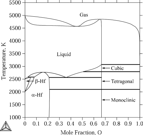
Figure 8: Calculated Hf-O phase diagram.

In the present work, the ternary liquid phase is extrapolated from the binaries. The enthalpy of formation of HfSiO₄ is obtained from first-principles calculations and the entropy of formation is evaluated from its preitectic reaction, Liquid + HfO₂ (Monoclinic) $\rightarrow$ $\rm HfSiO_{4}$, at 2023K as reported by Parfenenko et al[20]. The pseudo-binary phase diagram of HfO₂-SiO₂ is calculated and shown in Fig. 9.

Figure 9: Calculated HfO₂-SiO₂ pseudo-binary phase diagram.

As discussed in the introduction, HfO₂ is a promising candidate to replace SiO₂ as the gate dielectric in CMOS transistors due to its high dielectric constant and compatibility with Si in comparison with ZrO₂[5]. In general, during the fabrication of such devices, the films are subjected to temperatures around 1273K for a short period of time[4]. Thus, it is quite essential to understand the thermodynamic stability of HfO₂/SiO₂/Si.

From the evaluated thermodynamic database of the Hf-Si-O, the isothermal sections of the Hf-Si-O system can be readily calculated to study the stability of the HfO₂/Si interface. Two different temperatures are selected for the calculations and they are 500K for low temperature processing, such as mist deposition method and rapid thermal processing[40] and 1000K, typical temperature for the epitaxial growth of oxides deposition. Calculated isothermal sections of the Hf-Si-O system at 500K and 1000K are shown in Fig. 10(a) and 10(b), respectively. The two three-phase regions, HfSiO₄+HfO₂+Hf₂Si and HfSiO₄+diamond+Hf₂Si, in the 500K isothermal section should be noticed with respect to the stability of HfO₂/Si interface. Since those regions are intersected by the line connecting HfO₂ and Si, HfSi₂ can be found in the fabrication of polySi/HfO₂ gate stack Metal Oxide Semiconductor Field Effect Transistor (MOSFET) on bulk Si at 500K, while the 1000K calculation result clearly shows that HfO₂ is stable with the Si substrate.

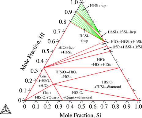
(a) 500K

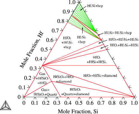
(b) 1000K

Figure 10: Calculated isothermal section of Hf-Si-O at (a) 500K and (b) 1000K at 1 atm. Tie lines are drawn inside the two phase regions. The vertical cross section between HfO₂ and Si is the isopleth in Figure 11.

A vertical cross section of isothermal sections, the isopleth between HfO₂-Si is calculated in order to investigate the stability range of HfSi₂ in the HfO₂/Si interface and is given in Fig. 11. It should be noted that HfSiO₄ at the low temperature range is zero amount. The calculated result shows that HfSi₂ becomes stable below 543.53K. This result is in agreement with the experimental observation from Gutowski et al[5]. Their HfO₂ film was deposited at 823K and then annealed at 1023K without the formation of any silicides.

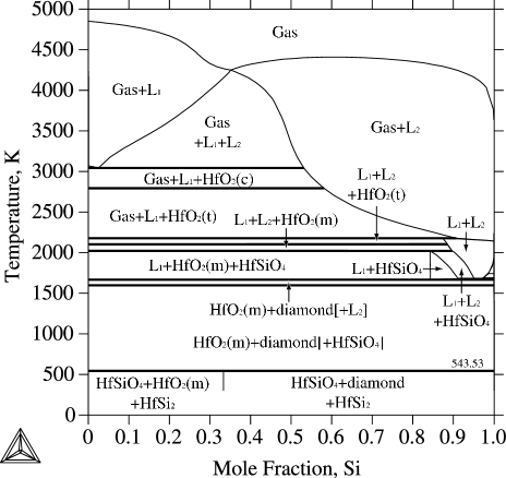
Figure 11: Calculated isopleth of HfO₂-Si at 1 atm. Hafnium dioxide is left and silicon is right. Polymorphs of HfO₂, monoclinic, tetragonal, and cubic, are given in parentheses. The phases in the bracket are zero amount.

It should be emphasized that the thermodynamic stability of HfSi₂ in the HfO₂/Si interface depends on the formation energy of HfSiO₄ based on the isothermal sections and the isopleth calculations. The enthalpy of formation for HfSiO₄ is calculated from first-principles calculations since there is no experimental measurement. To further illustrate this, the reference states of the enthalpy of formation for HfSiO₄ are defined as the two binary metal oxides (See Eqn. 11 and Table 1).

$$\Delta H^{HfSiO_{4}}_{f}=H(HfSiO_{4})-\tfrac{1}{2}H(HfO_{2})-\tfrac{1}{2}H(SiO_{2})$$ (11)

The current result of the HfSiO₄ calculation predicts that HfSi₂ is stable up to 543.53K. However, the uncertainty of the formation enthalpy of HfSiO₄, which originates from the density functional theory itself, is about $\pm$1 kJ/mol-atom[41]. Thus, the associated decomposition temperature of HfSi₂ in the HfO₂/Si interface varies from 381.92K to 669.76K within the calculated uncertainty of HfSiO₄. The recent work from Miyata et al. [42] found the formation of nanometer-scale HfSi₂ dots on the newly opened void surface produced by the decomposition of HfO₂/SiO₂ films at the oxide/void boundary in vacuum. However, their result cannot be directly compared with the current thermodynamic calculations due to the unknown oxygen partial pressure.

All parameters for the Hf-Si-O system are listed in Table 8.

Table 8: Thermodynamic parameters of the Hf-Si-O ternary system (in S.I. units). Gibbs energies for pure elements and gas phases are respectively from the SGTE pure elements database[44] and the SSUB database[36].

Phase	Sublattice model	Evaluated description
Ionic	$\rm(Hf^{+4})_{p}(O^{-2},Va)_{q}$	$\rm{}^{0}G^{Ionic~{}liquid}_{Hf^{+4}:O^{-2}}=2G^{monoclinic}_{HfO_{2}}+252000-86.798T$
liquid		$\rm{}^{0}G^{Ionic~{}liquid}_{Hf^{+4}:Va}={}^{0}G^{Liquid}_{Hf}$
		$\rm{}^{0}L^{Ionic~{}liquid}_{Hf^{+4}:O^{-2},Va}=50821+4.203T$
		$\rm{}^{1}L^{Ionic~{}liquid}_{Hf^{+4}:O^{-2},Va}=420485-133.300T$
		$\rm{}^{2}L^{Ionic~{}liquid}_{Hf^{+4}:O^{-2},Va}=30537$
hcp	$\rm(Hf)_{1}(O,Va)_{0.5}$	$\rm{}^{0}G^{hcp}_{Hf:Va}={}^{0}G^{hcp}_{Hf}$
		$\rm{}^{0}G^{hcp}_{Hf:O}={}^{0}G^{hcp}_{Hf}+0.5{}^{0}G^{Gas}_{O}-271214+41.560T$
		$\rm{}^{0}L^{hcp}_{Hf:O,Va}=-31345$
		$\rm{}^{1}L^{hcp}_{Hf:O,Va}=-6272$
bcc	$\rm(Hf)_{1}(O,Va)_{3}$	$\rm{}^{0}G^{bcc}_{Hf:Va}={}^{0}G^{bcc}_{Hf}$
		$\rm{}^{0}G^{bcc}_{Hf:O}={}^{0}G^{hcp}_{Hf}+3{}^{0}G^{Gas}_{O}-737857+268.540T$
		$\rm{}^{0}L^{hcp}_{Hf:O,Va}=-981440+20.349T$
HfSiO4	$\rm(Hf)_{1}(Si)_{1}(O)_{4}$	$\rm{}^{0}G^{HfSiO_{4}}_{Hf:Si:O}=G^{monoclinic}_{HfO_{2}}+G^{quartz}_{SiO_{2}}-10615+1.313T$

6 Summary and conclusion

The complete thermodynamic description of the Hf-Si-O ternary system is developed via the hybrid approach of first-principles calculations and CALPHAD modeling in the present work. In the Hf-O system, special quasirandom structures have been generated to calculate the enthalpies of mixing of oxygen and vacancies in the $\alpha$ and $\beta$ solid solutions. Calculated enthalpies of mixing of $\alpha$-Hf are almost identical to the model-calculated value whereas those of $\beta$-Hf show significant discrepancy. In the $\beta$ phase, first-principles calculations could not retain its original symmetry as bcc due to the strong interaction between the atoms in the structure. The calculated enthalpies of mixing from SQS’s results are combined with the enthalpies of formations of those hypothetical compounds calculated from the electronic structure calculations to derive the Gibbs energy of solid solutions in the Hf-O system.

In the total energy calculation of oxygen gas, vibrational, rotational and translational degrees of freedom are considered. With the adjusted total energy of oxygen molecule, the enthalpies of formation from first-principles calculations for both ordered and disordered phases showed good agreement with evaluated values.

The Hf-O system has been combined with the Hf-Si and the Si-O systems to calculate the Hf-Si-O ternary system with the ternary compound HfSiO₄ introduced from the first-principles calculations. From the Hf-Si-O thermodynamic database, phase stabilities pertinent to thin film processing such as HfO₂-SiO₂ pseudo-binary, isothermal sections, and isopleth have been calculated. The thermodynamic calculation results show that the HfO₂/Si interface is stable above 543.53K, which agrees with previous experimental results. However, due to the uncertainty of HfSiO₄ formation energy from first-principles, the stability of HfSi₂ in the HfO₂/Si interface is still in question and further experimental investigation is required.

It can be concluded that the thermodynamic properties of solid phases can be obtained from first-principles calculations not only for the ordered structures but also for the solution phases as long as one can find appropriate geometrical input for phases of interest. Special quasirandom structures for a substitutional solution phase is one example. However, one should notice that such a supercell only mimics short-ranged interaction as in metallic alloy systems. As shown in the present work, SQS’s can successfully describe the mixing behavior between oxygen and vacancies in the $\alpha$ solid solution where oxygen concentrations are relatively low, but for the oxygen-rich $\beta$ phase such interactions between the electrons at the longer distance become important and lead to the collapse of its original structure as bcc when the structure has been fully relaxed.

References

- Komarek et al. [1981] K. L. Komarek, P. J. Spencer, and International Atomic Energy Agency. Hafnium : physico-chemical properties of its compounds and alloys. Atomic Energy Review Special issue ; no 8. International Atomic Energy Agency, Vienna, 1981.
- Sayan et al. [2003] S. Sayan, E. Garfunkel, T. Nishimura, W. H. Schulte, T. Gustafsson, and G. D. Wilk. J. Appl. Phys., 94(2):928–934, 2003.
- Hubbard and Schlom [1996] K. J. Hubbard and D. G. Schlom. J. Mater. Res., 11(11):2757–2776, 1996.
- Ramanathan et al. [2003] Shriram Ramanathan, Paul C. McIntyre, Jan Luning, Patrick S. Lysaght, Yan Yang, Zhiqiang Chen, and Susanne Stemmer. J. Electrochem. Soc., 150(10):F173–F177, 2003.
- Gutowski et al. [2002] Maciej Gutowski, John E. Jaffe, Chun-Li Liu, Matt Stoker, Rama I. Hegde, Raghaw S. Rai, and Philip J. Tobin. Appl. Phys. Lett., 80(11):1897–1899, 2002.
- Waldner and Eriksson [1999] Peter Waldner and Gunnar Eriksson. CALPHAD, 23(2):189–218, 1999.
- Wang et al. [2005] Chong Wang, Matvei Zinkevich, and Fritz Aldinger. CALPHAD, 28(3):281–292, 2005.
- Rudy and Stecher [1963] E. Rudy and P. Stecher. Journal of the Less-Common Metals, 5(No. 1):78–89, 1963.
- Domagala and Ruh [1965] R. F. Domagala and Robert Ruh. Am. Soc. Metals, Trans. Quart., 58(2):164–75, 1965.
- Ruda et al. [1976] G. I. Ruda, V. V. Vavilova, I. I. Kornilov, L. E. Fykin, and L. D. Panteleev. Izvestiya Akademii Nauk SSSR, Neorganicheskie Materialy, 12(3):461–5, 1976.
- Ruh and Patel [1973] Robert Ruh and Vinod A. Patel. J. Am. Ceram. Soc., 56(11):606–7, 1973.
- Geller and Corenzwit [1953] S. Geller and E. Corenzwit. Anal. Chem., 25:1774, 1953.
- Curtis et al. [1954] C. E. Curtis, L. M. Doney, and J. R. Johnson. J. Am. Ceram. Soc., 37:458–65, 1954.
- Adam and Rogers [1959] J. Adam and M. D. Rogers. Acta Cryst., 12:951, 1959.
- Boganov et al. [1965] A. G. Boganov, V. S. Rudenko, and L. P. Makarov. Doklady Akademii Nauk SSSR, 160(5):1065–8, 1965.
- Stacy and Wilder [1975] D. W. Stacy and D. R. Wilder. J. Am. Ceram. Soc., 58(7-8):285–8, 1975.
- Wang et al. [1992] J. Wang, H. P. Li, and R. Stevens. J. Mater. Sci., 27(20):5397–430, 1992.
- Massalski [1990] T. B. Massalski. Binary alloy phase diagrams. Binary alloy phase diagrams. ASM International, Materials Park, Ohio, 2nd edition, 1990.
- Speer and Cooper [1982] J. Alexander Speer and Brian J. Cooper. Am. Mineral., 67(7-8):804–8, 1982.
- Parfenenkov et al. [1969] V. N. Parfenenkov, R. G. Grebenshchikov, and N. A. Toropov. Doklady Akademii Nauk SSSR, 185(4):840–2, 1969.
- Hirabayashi et al. [1973] Makoto Hirabayashi, Sadae Yamaguchi, and Tetsuji Arai. J. Phys. Soc. Jpn., 35(2):473–81, 1973.
- Boureau and Gerdanian [1984] G. Boureau and P. Gerdanian. J. Phys. Chem. Solids, 45(2):141–5, 1984.
- Komarek and Silver [1963] K. L. Komarek and M. Silver. Thermodynamics of Nuclear Materials, Proceedings of the Symposium on Thermodynamics of Nuclear Materials, 1962:749–73, 1963.
- Silver et al. [1963] M. D. Silver, P. A. Farrar, and Kurt L. Komarek. Transactions of the American Institute of Mining, Metallurgical and Petroleum Engineers, 227(4):876–84, 1963.
- Kresse and Furthmuller [1996] G. Kresse and J. Furthmuller. Comput. Mater. Sci., 6(1):15–50, 1996.
- Kresse and Joubert [1999] G. Kresse and D. Joubert. Phys. Rev. B, 59(3):1758–1775, 1999.
- Perdew et al. [1992] John P. Perdew, J. A. Chevary, S. H. Vosko, Koblar A. Jackson, Mark R. Pederson, D. J. Singh, and Carlos Fiolhais. Phys. Rev. B, 46(11):6671–87, 1992.
- McQuarrie [2000] Donald A. McQuarrie. Statistical mechanics. Statistical mechanics. University Science Books, Sausalito, Calif., 2000.
- Zunger et al. [1990] Alex Zunger, S. H. Wei, L. G. Ferreira, and James E. Bernard. Phys. Rev. Lett., 65(3):353–6, 1990.
- Jiang et al. [2004] Chao Jiang, C. Wolverton, Jorge Sofo, Long-Qing Chen, and Zi-Kui Liu. Phys. Rev. B, 69(21):214202/1–214202/10, 2004.
- Shin et al. [2006] D. Shin, R. Arróyave, Z.-K. Liu, and A. van de Walle. Phys. Rev. B, 74(2):024204/1–024204/13, 2006.
- Tsuji [1997] Toshihide Tsuji. J. Nucl. Mater., 247:63–71, 1997.
- Arróyave et al. [2002] Raymundo Arróyave, Larry Kaufman, and Thomas W. Eagar. CALPHAD, 26(1):95–118, 2002.
- Redlich and Kister [1948] O. Redlich and A.T. Kister. Ind. Eng. Chem., 40(2):345–348, 1948.
- Hillert et al. [1985] Mats Hillert, Bo Jansson, Bo Sundman, and John Aagren. Metall. Trans. A, 16A(2):261–6, 1985.
- [36] Scientific Group Thermodata Europe (SGTE). Thermodynamic Properties of Inorganic Materials, volume 19 of Landolt-Boernstein New Series, Group IV. Springer, Verlag Berlin Heidelberg, 1999.
- Hallstedt [1992] Bengt Hallstedt. CALPHAD, 16(1):53–61, 1992.
- Zhao et al. [2000] J. C. Zhao, B. P. Bewlay, M. R. Jackson, and Q. Chen. J. Phase Equilib., 21(1):40–45, 2000.
- Andersson et al. [2002] J. O. Andersson, Thomas Helander, Lars Hoglund, Pingfang Shi, and Bo Sundman. CALPHAD, 26(2):273–312, 2002.
- Chang et al. [2004] K. Chang, K. Shanmugasundaram, D. O. Lee, P. Roman, C. T. Wu, J. Wang, J. Shallenberger, P. Mumbauer, R. Grant, R. Ridley, G. Dolny, and J. Ruzyllo. Microelectron. Eng., 72(1-4):130–135, 2004.
- Wolverton et al. [2002] C. Wolverton, X. Y. Yan, R. Vijayaraghavan, and V. Ozolins. Acta Mater., 50(9):2187–2197, 2002.
- Miyata et al. [2005] Noriyuki Miyata, Yukinori Morita, Tsuyoshi Horikawa, Toshihide Nabatame, Masakazu Ichikawa, and Akira Toriumi. Phys. Rev. B, 71(23):233302/1–233302/4, 2005.
- Dagerhamn [1961] Tore Dagerhamn. Acta Chem. Scand., 15:214–15, 1961.
- Dinsdale [1991] A. T. Dinsdale. CALPHAD, 15(4):317–425, 1991.