SENSITIVITY ANALYSIS OF THE ORTHOGLIDE,A 3-DOF TRANSLATIONAL PARALLEL KINEMATIC MACHINE

Abstract

In this paper, two complementary methods are introduced to analyze the sensitivity of a three degree-of-freedom (DOF) translational Parallel Kinematic Machine (PKM) with orthogonal linear joints: the Orthoglide. Although these methods are applied to a particular PKM, they can be readily applied to 3-DOF Delta-Linear PKM such as ones with their linear joints parallel instead of orthogonal. On the one hand, a linkage kinematic analysis method is proposed to have a rough idea of the influence of the length variations of the manipulator on the location of its end-effector. On the other hand, a differential vector method is used to study the influence of the length and angular variations in the parts of the manipulator on the position and orientation of its end-effector. Besides, this method takes into account the variations in the parallelograms. It turns out that variations in the design parameters of the same type from one leg to another have the same effect on the position of the end-effector. Moreover, the sensitivity of its pose to geometric variations is a minimum in the kinematic isotropic configuration of the manipulator. On the contrary, this sensitivity approaches its maximum close to the kinematic singular configurations of the manipulator.

Keywords: Parallel Kinematic Machine, Sensitivity Analysis, Kinematic Analysis, Kinematic Singularity, Isotropy.

${\cal R}_{b}(O,x,y,z)$

: reference coordinate frame centered at $O$, the intersection between the directions of the three actuated prismatic joints.

${\cal R}_{P}(P,X,Y,Z)$

: coordinate frame attached to the end-effector.

${\cal R}_{i}(A_{i},x_{i},y_{i},z_{i})$

: coordinate frame attached to the $i^{th}$ prismatic joint, $i=1,2,3$.

${\bf p}=\left[\begin{array}[]{ccc}p_{x}&p_{y}&p_{z}\end{array}\right]^{T}$

: vector of the Cartesian coordinates of the end-effector, expressed in ${\cal R}_{b}$.

$\delta{\bf p}=\left[\begin{array}[]{ccc}\delta p_{x}&\delta p_{y}&\delta p_{z}\end{array}\right]^{T}$

: position error of the end-effector, expressed in ${\cal R}_{b}$.

$\delta\theta=\left[\begin{array}[]{ccc}\delta\theta_{x}&\delta\theta_{y}&\delta\theta_{z}\end{array}\right]^{T}$

: orientation error of the end-effector, expressed in ${\cal R}_{b}$.

$\rho_{i}$

: displacement of the $i^{th}$ prismatic joint.

$\delta\rho_{i}$

: displacement error of the $i^{th}$ prismatic joint.

$L_{i}$

: theoretical length of the $i^{th}$ parallelogram.

$A_{i},B_{i},C_{i}$

: depicted in Fig. 1.

$a_{i}$

: distance between points $O$ and $A_{i}$.

$r_{i}$

: distance between points $P$ and $C_{i}$.

$b_{1y},b_{1z}$

: position errors of point $B_{1}$ along $y$ and $z$ axes, respectively.

$b_{2x},b_{2z}$

: position errors of point $B_{2}$ along $x$ and $z$ axes, respectively.

$b_{3x},b_{3y}$

: position errors of point $B_{3}$ along $x$ and $y$ axes, respectively.

$h_{1}=b_{1y},\ k_{1}=b_{1z},\ h_{2}=b_{2x},\ k_{2}=b_{2z},\ h_{3}=b_{3x},\ k_{3}=b_{3y}.$

$d_{i}$

: nominal width of the $i^{th}$ parallelogram.

$\delta L_{i}$

: variation in the length of the $i^{th}$ parallelogram.

$\delta L_{ij}$

: variation in the length of link $\overline{B_{ij}C_{ij}}$, $j=1,2$ (see Fig. 2).

$\delta b_{i}$

: variation in the length of link $\overline{B_{i1}B_{i2}}$.

$\delta c_{i}$

: variation in the length of link $\overline{C_{i1}C_{i2}}$.

$\delta l_{i}$

: parallelism error of links $\overline{B_{i1}B_{i2}}$ and $\overline{C_{i1}C_{i2}}$.

$\delta m_{i}$

: parallelism error of links $\overline{B_{i1}C_{i1}}$ and $\overline{B_{i2}C_{i2}}$.

${\bf w}_{i}$

: direction of links $\overline{B_{i1}C_{i1}}$ and $\overline{B_{i2}C_{i2}}$.

$\delta{\bf w}_{i}$

: variation in the direction of links $\overline{B_{i1}C_{i1}}$ and $\overline{B_{i2}C_{i2}}$.

$\delta{\bf e}_{i}$

: sum of the position errors of points $A_{i}$, $B_{i}$, $C_{i}$.

$\delta\boldsymbol{\theta}_{Ai}=\left[\begin{array}[]{ccc}\delta\theta_{Aix}&\delta\theta_{Aiy}&\delta\theta_{Aiz}\end{array}\right]^{T}$

: angular variation in the direction of the $i^{th}$ prismatic joint.

$\delta\theta_{Bi}=\left[\begin{array}[]{ccc}\delta\theta_{Bix}&\delta\theta_{Biy}&\delta\theta_{Biz}\end{array}\right]^{T}$

: angular variation between $\overline{B_{i1}B_{i2}}$ and the direction of the $i^{th}$ prismatic joint.

$\delta\theta_{Ci}=\left[\begin{array}[]{ccc}\delta\theta_{Cix}&\delta\theta_{Ciy}&\delta\theta_{Ciz}\end{array}\right]^{T}$

: angular variation between the end-effector and $\overline{C_{i1}C_{i2}}$.

$\delta{\gamma}_{i}=\left[\begin{array}[]{ccc}\delta{\gamma}_{ix}&\delta{\gamma}_{iy}&\delta{\gamma}_{iz}\end{array}\right]^{T}$

sum of the orientation errors of the $i^{th}$ parallelogram with respect to the $i^{th}$ prismatic joint and the end-effector.

DOF

: degree-of-freedom.

PKM

: parallel kinematic machine.

1 Introduction

For two decades, parallel manipulators have attracted the attention of more and more researchers who consider them as valuable alternative design for robotic mechanisms. As stated by numerous authors, conventional serial kinematic machines have already reached their dynamic performance limits, which are bounded by high stiffness of the machine components required to support sequential joints, links and actuators. Thus, while having good operating characteristics (large workspace, high flexibility and manoeuvrability), serial manipulators have disadvantages of low stiffness and low power. Conversely, parallel kinematic machines (PKM) offer essential advantages over their serial counterparts (lower moving masses, higher stiffness and payload-to-weight ratio, higher natural frequencies, better accuracy, simpler modular mechanical construction, possibility to locate actuators on the fixed base).

However, PKM are not necessarily more accurate than their serial counterparts. Indeed, even if the dimensional variations can be compensated with PKM, they can also be amplified contrary to with their serial counterparts, [1]. Wang et al. [2] studied the effect of manufacturing tolerances on the accuracy of a Stewart platform. Kim et al. [3] used a forward error bound analysis to find the error bound of the end-effector of a Stewart platform when the error bounds of the joints are given, and an inverse error bound analysis to determine those of the joints for the given error bound of the end-effector. Kim and Tsai [4] studied the effect of misalignment of linear actuators of a 3-DOF translational parallel manipulator on the motion of its moving platform. Han et al. [5] used a kinematic sensitivity analysis method to explain the gross motions of a 3-UPU parallel mechanism, and they showed that it is highly sensitive to certain minute clearances. Fan et al. [6] analyzed the sensitivity of the 3-PRS parallel kinematic spindle platform of a serial-parallel machine tool. Verner et al. [7] presented a new method for optimal calibration of PKM based on the exploitation of the least error sensitive regions in their workspace and geometric parameters space. As a matter of fact, they used a Monte Carlo simulation to determine and map the sensitivities to geometric parameters. Moreover, Caro et al. [8] developed a tolerance synthesis method for mechanisms based on a robust design approach.

This paper aims at analyzing the sensitivity of the Orthoglide to its dimensional and angular variations. The Orthoglide is a three degree-of-freedom (DOF) translational PKM developed by Chablat and Wenger [9]. A small-scale prototype of this manipulator was built at IRCCyN.

Here, the sensitivity of the Orthoglide is studied by means of two complementary methods. First, a linkage kinematic analysis is used to have a rough idea of the influence of the dimensional variations to its end-effector and to show that the variations in design parameters of the same type from one leg to another have the same influence on the location of the end-effector. Although this method is compact, it cannot be used to know the influence of the variations in the parallelograms. Thus, a differential vector method is developed to study the influence of the dimensional and angular variations in the parts of the manipulator, and particularly variations in the parallelograms, on the position and the orientation of its end-effector.

In the isotropic kinematic configuration, the end-effector of the manipulator is located at the intersection between the directions of its three actuated prismatic joints, and the condition number of its kinematic Jacobian matrix is equal to one, [10]. It is shown that this configuration is the least sensitive one to geometrical variations, contrary to the closest configurations to its kinematic singular configurations, which are the most sensitive to geometrical variations.

Although the two sensitivity analysis methods are applied to a particular PKM, these methods can be readily applied to other 3-DOF Delta-linear PKM such as ones with parallel linear joints instead of orthogonal ones.

2 Manipulator Geometry

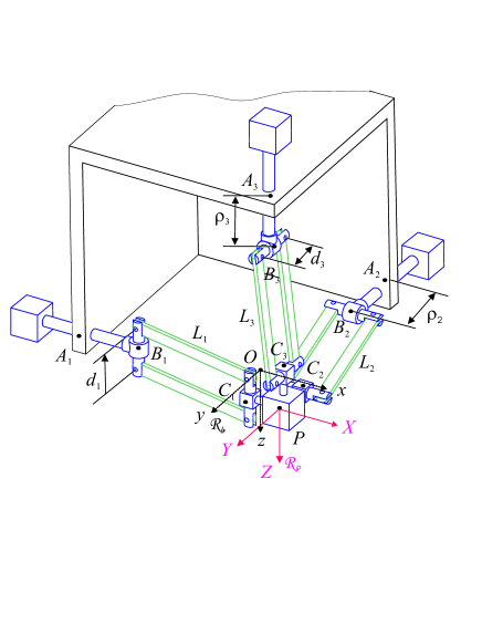
Figure 1: Basic kinematic architecture of the Orthoglide

The kinematic architecture of the Orthoglide is shown in Fig.1. It consists of three identical parallel chains that are formally described as PR$\mbox{P}_{a}$RR, where P, R and $\mbox{P}_{a}$ denote the prismatic, revolute, and parallelogram joints respectively, as shown in Fig.2.

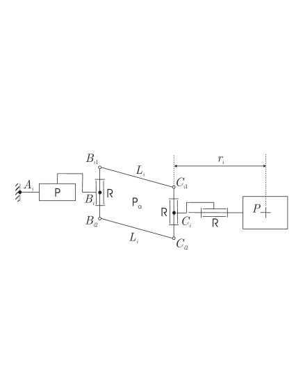
Figure 2: Morphology of the $i^{th}$ leg of the Orthoglide

The mechanism input is made up of three actuated orthogonal prismatic joints. The output body (with a tool mounting flange) is connected to the prismatic joints through a set of three kinematic chains. Inside each chain, one parallelogram is used and oriented in a manner that the output body is restricted to translational movements only.

The small-scale prototype of the Orthoglide was designed to reach Cartesian velocity of 1.2 m/s and an acceleration of 17 m/s². The desired payload is 4 kg (spindle, tool, included). The size of its prescribed cubic workspace, $C_{u}$, is $200\times 200\times 200$ mm, where the velocity transmission factors are bounded between $1/2$ and $2$. The three legs are supposed to be identical. According to [9], the nominal lengths, $L_{i}$, and widths, $d_{i}$, of the parallelograms, and the nominal distances, $r_{i}$, between points $C_{i}$ and the end-effector $P$ are identical, i.e.: $L=L_{1}=L_{2}=L_{3}=310.58$ mm, $d=d_{1}=d_{2}=d_{3}=80$ mm, $r=r_{1}=r_{2}=r_{3}=31$ mm.

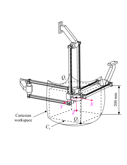
Figure 3: Cartesian workspace, $C_{u}$, points $Q_{1}$ and $Q_{2}$

As depicted in Fig.3, $Q_{1}$ and $Q_{2}$, vertices of $C_{u}$, are defined at the intersection between the Cartesian workspace boundary and the axis $x=y=z$ expressed in the reference coordinate frame ${\cal R}_{b}$. $Q_{1}$ and $Q_{2}$ are the closest points to the singularity surfaces. Their Cartesian coordinates, expressed in ${\cal R}_{b}$, are equal to (-73.21,-73.21,-73.21) and (126.79,126.79,126.79), respectively.

The parts of the manipulator are supposed to be rigid-bodies and there is no joint clearance. The legs of the manipulator, composed of one prismatic joint, one parallelogram, and three revolute joints, generate a five DOF motion each. Besides, they are identical. Therefore, according to Karouia et al. [11], the manipulator is isostatic. Thus, the results obtained by the sensitivity analysis methods developed in this paper are meaningful.

3 Sensitivity Analysis

Two complementary methods are used to study the sensitivity of the Orthoglide. First, a linkage kinematic analysis is used to have a rough idea of the influence of the dimensional variations to its end-effector. Although this method is compact, it cannot be used to know the influence of the variations in the parallelograms. Thus, a differential vector method is used to study the influence of the dimensional and angular variations in the parts of the manipulator, and particularly variations in the parallelograms, on the position and the orientation of its end-effector.

3.1 Linkage Kinematic Analysis

This method aims at computing the sensitivity coefficients of the position of the end-effector, $P$, to the design parameters of the manipulator. First, three implicit functions depicting the kinematic of the manipulator are obtained. A relation between the variations in the position of $P$ and the variations in the design parameters follows from these functions. Finally a sensitivity matrix, which gathers the sensitivity coefficients of $P$, follows from the previous relation written in matrix form.

3.1.1 Formulation

Figure 1 depicts the design parameters taken into account. Points $A_{1}$, $A_{2}$, and $A_{3}$ are the bases of the prismatic joints. Their Cartesian coordinates, expressed in ${\cal R}_{b}$, are ${\bf a}_{1}$, ${\bf a}_{2}$, and ${\bf a}_{3}$, respectively.

$${\bf a}_{1}=\left[\begin{array}[]{ccc}-a_{1}&0&0\end{array}\right]^{T}$$ (1b)

$${\bf a}_{2}=\left[\begin{array}[]{ccc}0&-a_{2}&0\end{array}\right]^{T}$$ (1d)

$${\bf a}_{3}=\left[\begin{array}[]{ccc}0&0&-a_{3}\end{array}\right]^{T}$$ (1f)

where $a_{i}$ is the distance between points $A_{i}$ and $O$, the origin of ${\cal R}_{b}$. Points $B_{1}$, $B_{2}$ and $B_{3}$ are the links between the prismatic and parallelogram joints. Their Cartesian coordinates, expressed in ${\cal R}_{b}$ are:

$${\bf b}_{1}=\left[\begin{array}[]{c}-a_{1}+\rho_{1}\\ b_{1y}\\ b_{1z}\end{array}\right]$$ (2d)

$${\bf b}_{2}=\left[\begin{array}[]{c}b_{2x}\\ -a_{2}+\rho_{2}\\ b_{2z}\end{array}\right]$$ (2h)

$${\bf b}_{3}=\left[\begin{array}[]{c}b_{3x}\\ b_{3y}\\ -a_{3}+\rho_{3}\end{array}\right]$$ (2l)

where $\rho_{i}$ is the displacement of the $i^{th}$ prismatic joint. $b_{1y}$ and $b_{1z}$ are the position errors of point $B_{1}$ according to $y$ and $z$ axes. $b_{2x}$ and $b_{2z}$ are the position errors of point $B_{2}$ according to $x$ and $z$ axes. $b_{3x}$ and $b_{3y}$ are the position errors of point $B_{3}$ according to $x$ and $y$ axes. These errors result from the orientation errors of the directions of the prismatic actuated joints. The Cartesian coordinates of $C_{1}$, $C_{2}$, and $C_{3}$, expressed in ${\cal R}_{b}$, are the following:

$${\bf c}_{1}=\left[\begin{array}[]{ccc}p_{x}-r_{1}&0&0\end{array}\right]^{T}$$ (3b)

$${\bf c}_{2}=\left[\begin{array}[]{ccc}0&p_{y}-r_{2}&0\end{array}\right]^{T}$$ (3d)

$${\bf c}_{3}=\left[\begin{array}[]{ccc}0&0&p_{z}-r_{3}\end{array}\right]^{T}$$ (3f)

where ${\bf p}={\left[\begin{array}[]{ccc}p_{x}&p_{y}&p_{z}\end{array}\right]}^{T}$ is the vector of the Cartesian coordinates of the end-effector $P$, expressed in ${\cal R}_{b}$.

The expressions of the nominal lengths of the parallelograms follow from eq.(4),

$$L_{i}=\|{\bf c}_{i}-{\bf b}_{i}\|_{2}\ ,\ i=1,2,3$$ (4)

where $L_{i}$ is the nominal length of the $i^{th}$ parallelogram and $\|.\|_{2}$ is the Euclidean norm. Three implicit functions follow from eq.(4) and are given by the following equations:

$$F_{1} = (-r_{1}+p_{x}+a_{1}-\rho_{1})^{2}+(p_{y}-b_{1y})^{2}+(p_{z}-b_{1z})^{2}-L_{1}^{2}=0$$

$$F_{2} = (p_{x}-b_{2x})^{2}+(-r_{2}+p_{y}+a_{2}-\rho_{2})^{2}+(p_{z}-b_{2z})^{2}-L_{2}^{2}=0$$

$$F_{3} = (p_{x}-b_{3x})^{2}+(p_{y}-b_{3y})^{2}+(-r_{3}+p_{z}+a_{3}-\rho_{3})^{2}-L_{3}^{2}=0$$

By differentiating functions $F_{1}$, $F_{2}$, and $F_{3}$, with respect to the design parameters of the manipulator and the position of the end-effector, we obtain a relation between the positioning error of the end-effector, $\delta{\bf p}$, and the variations in the design parameters, $\delta{\bf q}_{i}$.

$${\delta F}_{i}={\bf A}_{i}\delta{\bf p}+{\bf B}_{i}\delta{\bf q}_{i}=0\ ,\ i=1,2,3$$ (5)

with

$${\bf A}_{i} = \left[\begin{array}[]{ccc}{\partial F_{i}}/{\partial p_{x}}&{\partial F_{i}}/{\partial p_{y}}&{\partial F_{i}}/{\partial p_{z}}\end{array}\right]$$ (7)

$${\bf B}_{i} = \left[\begin{array}[]{cccccc}{\partial F_{i}}/{\partial a_{i}}&{\partial F_{i}}/{\partial b_{iy}}&{\partial F_{i}}/{\partial b_{iz}}&{\partial F_{i}}/{\partial\rho_{i}}&{\partial F_{i}}/{\partial L_{i}}&{\partial F_{i}}/{\partial r_{i}}\end{array}\right]$$ (9)

$$\delta{\bf p} = {\left[\begin{array}[]{ccc}\delta p_{x}&\delta p_{y}&\delta p_{z}\end{array}\right]}^{T}$$ (11)

$$\delta{\bf q}_{i} = \left[\begin{array}[]{cccccc}{\delta a_{i}}&{\delta h_{i}}&{\delta k_{i}}&{\delta\rho_{i}}&{\delta L_{i}}&{\delta r_{i}}\end{array}\right]^{T}$$ (13)

where ${\delta a_{i}}$, ${\delta h_{i}}$, ${\delta k_{i}}$, ${\delta\rho_{i}}$, ${\delta L_{i}}$, and ${\delta r_{i}}$, depict the variations in $a_{i}$, $h_{i}$, $k_{i}$, $\rho_{i}$, $L_{i}$, and $r_{i}$, respectively with $h_{1}=b_{1y}$, $k_{1}=b_{1z}$, $h_{2}=b_{2x}$, $k_{2}=b_{2z}$, $h_{3}=b_{3x}$, $k_{3}=b_{3y}$.

Integrating the three loops of eq.(5) together and separating the position parameters and design parameters to different sides yields the following simplified matrix form:

$${\bf A}\delta{\bf p}+{\bf B}\delta{\bf q}=0$$ (14)

with

$${\bf A} = {\left[\begin{array}[]{ccc}{\bf A}_{1}^{T}{\bf A}_{2}^{T}{\bf A}_{3}^{T}\end{array}\right]}^{T}\in{\mathbb{R}}^{3\times 3}$$ (16)

$${\bf B} = \left[\begin{array}[]{ccc}{\bf B}_{1}&0&0\\ 0&{\bf B}_{2}&0\\ 0&0&{\bf B}_{3}\end{array}\right]\in{\mathbb{R}}^{3\times 18}$$ (20)

$$\delta{\bf q} = \left[\begin{array}[]{ccc}\delta{\bf q}_{1}^{T}&\delta{\bf q}_{2}^{T}&\delta{\bf q}_{3}^{T}\end{array}\right]^{T}\in{\mathbb{R}}^{18\times 1}$$ (22)

Equation (14) takes into account the coupling effect of the three independent structure loops. According to [9], A is the parallel Jacobian kinematic matrix of the Orthoglide, which does not meet parallel kinematic singularities when its end-effector covers $C_{u}$. Therefore, A is not singular and its inverse, ${\bf A}^{-1}$, exists. Thus, the positioning error of the end-effector can be computed using eq.(23).

$$\delta{\bf p}={\bf C}\ \delta{\bf q}$$ (23)

where

$${\bf C}=-{\bf A}^{-1}{\bf B}=\left[\begin{array}[]{ccccc}\partial p_{x}/\partial a_{1}&\partial p_{x}/\partial h_{1}&\cdots&\partial p_{x}/\partial r_{3}\\ \partial p_{y}/\partial a_{1}&\partial p_{y}/\partial h_{1}&\cdots&\partial p_{y}/\partial r_{3}\\ \partial p_{z}/\partial a_{1}&\partial p_{z}/\partial h_{1}&\cdots&\partial p_{z}/\partial r_{3}\end{array}\right]\in{\mathbb{R}}^{3\times 18}$$ (24)

represents the sensitivity matrix of the manipulator. The terms of ${\bf C}$ are the sensitivity coefficients of the Cartesian coordinates of the end-effector to the design parameters and are used to analyze the sensitivity of the Orthoglide.

3.1.2 Results of the Linkage Kinematic Analysis

The sensitivity matrix ${\bf C}$ of the manipulator depends on the position of its end-effector.

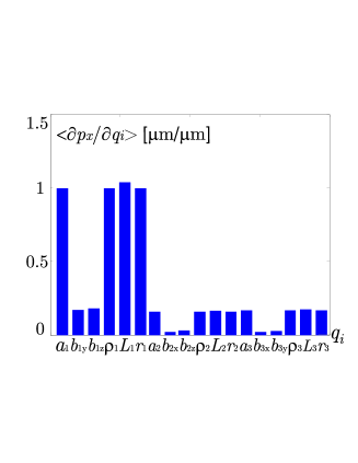
Figure 4: Mean of sensitivity of $p_{x}$ throughout $C_{u}$

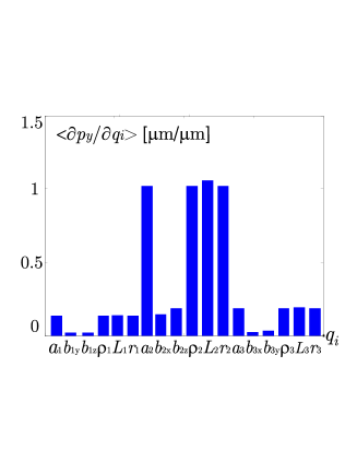
Figure 5: Mean of sensitivity of $p_{y}$ throughout $C_{u}$

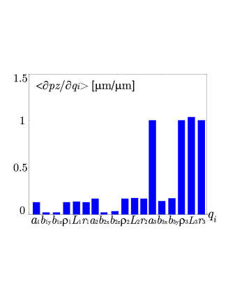
Figure 6: Mean of sensitivity of $p_{z}$ throughout $C_{u}$

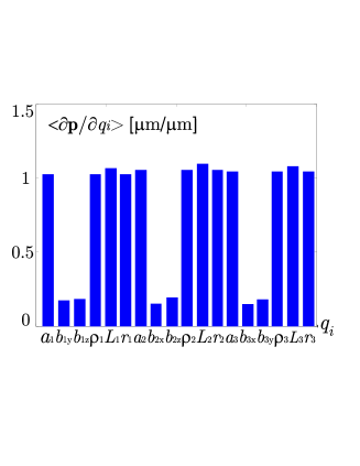
Figure 7: Mean of sensitivity of p throughout $C_{u}$

Figures 4, 5, 6 and 7 depict the mean of the sensitivity coefficients of $p_{x}$, $p_{y}$, $p_{z}$, and ${\bf p}$, when the end-effector covers $C_{u}$. It appears that the position of the end-effector is very sensitive to variations in the position of points $A_{i}$, variations in the lengths of the parallelograms, $L_{i}$, variations in the lengths of prismatic joints, $\rho_{i}$, and variations in the position of points $C_{i}$ defined by $r_{i}$ (see Fig.2). However, it is little sensitive to the orientation errors of the direction of the prismatic joints, defined by parameters $b_{1y},b_{1z},b_{2x},b_{2z},b_{3x},b_{3y}$. Besides, it is noteworthy that $p_{x}$ ($p_{y}$ , $p_{z}$, respectively) is very sensitive to the design parameters which make up the $1^{st}$ ($2^{nd}$, $3^{rd}$, respectively) leg of the manipulator, contrary to the others. That is due to the symmetry of the architecture of the manipulator. Henceforth, only the variations in the design parameters of the first leg of the manipulator will be taken into account. Indeed, the sensitivity of the position of the end-effector to the variations in the design parameters of the second and the third legs of the manipulator can be deduced from the sensitivity of the position of the end-effector to variations in the design parameters of the first leg.

Chablat et al. [9] showed that if the prescribed bounds of the velocity transmission factors (the kinematic criteria used to dimension the manipulator) are satisfied at $Q_{1}$ and $Q_{2}$, then these bounds are satisfied throughout the prescribed cubic Cartesian workspace $C_{u}$. $Q_{1}$ and $Q_{2}$ are then the most critical points of $C_{u}$, whereas $O$ is the most interesting point because it corresponds to the isotropic kinematic configuration of the manipulator. Here, we assume that if the prescribed bounds of the sensitivity coefficients are satisfied at $Q_{1}$ and $Q_{2}$, then these bounds are satisfied throughout $C_{u}$.

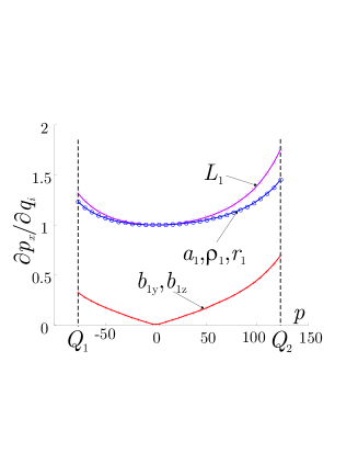
Figure 8: Sensitivity of $p_{x}$ to the variations in the $1^{st}$ leg

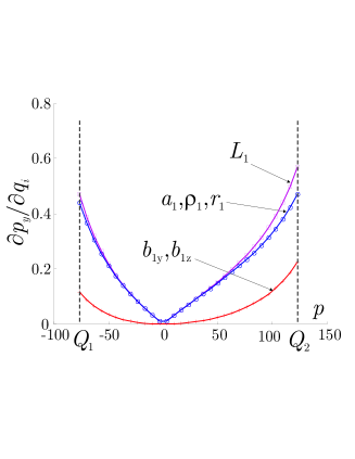
Figure 9: Sensitivity of $p_{y}$ to the variations in the $1^{st}$ leg

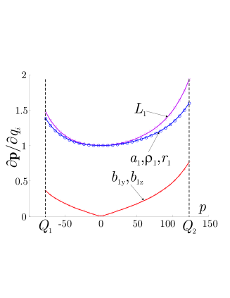
Figure 10: Sensitivity of ${\bf p}$ to the variations in the $1^{st}$ leg

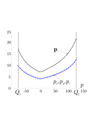
Figure 11: Global sensitivity of ${\bf p}$, $p_{x}$, $p_{y}$, and $p_{z}$

Figures 8 and 9 depict the sensitivity coefficients of $p_{x}$ and $p_{y}$ to the dimensional variations in the $1^{st}$ leg, i.e.: $a_{1},b_{1y},b_{1z},\rho_{1},L_{1},r_{1}$, along $Q_{1}Q_{2}$. It appears that these coefficients are a minimum in the isotropic configuration, i.e.: $P\equiv O$, and a maximum when $P\equiv Q_{2}$, i.e.: in the closest configuration to the singular one. Figure 10 depicts the sensitivity coefficients of ${\bf p}$ along diagonal $Q_{1}Q_{2}$. It is noteworthy that all the sensitivity coefficients are a minimum when $P\equiv O$ and a maximum when $P\equiv Q_{2}$. Finally, figure 11 depicts the global sensitivities of $\bf p$, $p_{x}$, $p_{y}$, and $p_{z}$ to the dimensional variations. It appears that they are a minimum when $P\equiv O$, and a maximum when $P\equiv Q_{2}$.

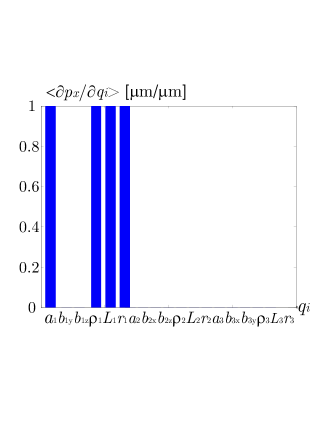
Figure 12: Sensitivity of $p_{x}$ in the isotropic configuration

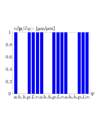
Figure 13: Sensitivity of $\bf p$ in the isotropic configuration

Figures 12 and 13 depict the sensitivity coefficients of $p_{x}$ and $\bf p$ in the isotropic configuration. In this configuration, the position error of the end-effector does not depend on the orientation errors of the directions of the prismatic joints because the sensitivity of the position of $P$ to variations in $b_{1y},b_{1z},b_{2x},b_{2z},b_{3x},b_{3y}$ is null in this configuration. Besides, variations in $p_{x}$, $p_{y}$, and $p_{z}$ are decoupled in this configuration. Indeed, variarions in $p_{x}$, ($p_{y}$, $p_{z}$, respectively) are only due to dimensional variations in the $1^{st}$, ($2^{nd}$, $3^{rd}$, respectively) leg of the manipulator. The corresponding sensitivity coefficients are equal to 1. It means that the dimensional variations are neither amplified nor compensated in the isotropic configuration.

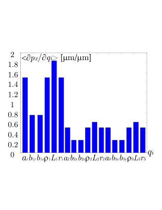
Figure 14: $Q_{2}$ configuration, sensitivity of $p_{x}$

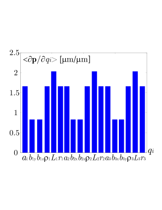
Figure 15: $Q_{2}$ configuration, sensitivity of ${\bf p}$

Figures 14 and 15 depict the sensitivity coefficients of $p_{x}$ and $\bf p$ when the end-effector hits $Q_{2}$ ($P\equiv Q_{2}$). In this case, variations in $p_{x}$, $p_{y}$, and $p_{z}$ are coupled. For example, variations in $p_{x}$ are due to both dimensional variations in the $1^{st}$ leg and variations in the $2^{nd}$ and the $3^{rd}$ legs. Besides, the amplification of the dimensional variations is important. Indeed, the sensitivity coefficients of $\bf p$ are close to 2 in this configuration. For example, as the sensitivity coefficient relating to $L_{1}$ is equal to 1.9, the position error of the end-effector will be equal to $19\mu m$ if $\delta L_{1}=10\mu m$. Moreover, we noticed numerically that $Q_{2}$ configuration is the most sensitive configuration to dimensional variations of the manipulator.

According to figures 4 - 7, 12 - 15, variations in design parameters of the same type from one leg to another have the same influence on the location of the end-effector.

However, this linkage kinematic method does not take into account variations in the parallelograms, except the variations in their global length. Thus, a differential vector method is developed below.

3.2 Differential Vector Method

In this section, we perfect a sensitivity analysis method of the Orthoglide, which complements the previous one. This method is used to analyze the sensitivity of the position and the orientation of the end-effector to dimensional and angular variations, and particularly to the variations in the parallelograms. Moreover, it allows us to distinguish the variations which are responsible for the position errors of the end-effector from the ones which are responsible for its orientation errors. To develop this method, we were inspired by a Huang & al. work on a parallel kinematic machine, which is made up of parallelogram joints too [12].

First, we express the dimensional and angular variations in vectorial form. Then, a relation between the position and the orientation errors of the end-effector is obtained from the closed-loop kinematic equations. The expressions of the orientation and the position errors of the end-effector, with respect to the variations in the design parameters, are deduced from this relation. Finally, we introduce two sensitivity indices to assess the sensitivity of the position and the orientation of the end-effector to dimensional and angular variations, and particularly to the parallelism errors of the bars of the parallelograms.

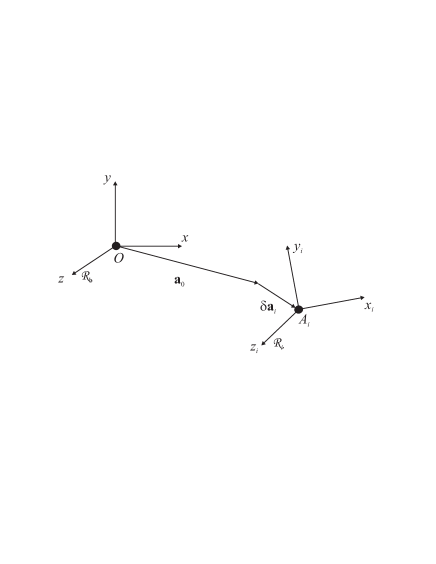
Figure 16: Variations in $O-A_{i}$ chain

3.2.1 Formulation

The schematic drawing of the $i^{th}$ leg of the Orthoglide depicted in Fig.2 is split in order to depict the variations in design parameters in a vectoriel form. The closed-loop kinematic chains $O-A_{i}-B_{i}-B_{ij}-C_{ij}-C_{i}-P$, $i=1,2,3$, $j=1,2$, are depicted by Figs.16-19. ${\cal R}_{i}$ is the coordinate frame attached to the $i^{th}$ prismatic joint. ${\bf o},{\bf a}_{i},{\bf b}_{i},{\bf b}_{ij},{\bf c}_{ij},{\bf c}_{i},{\bf p}$, are the Cartesian coordinates of points $O,A_{i},B_{i},B_{ij},C_{ij},C_{i},P$, respectively, expressed in ${\cal R}_{i}$ and depicted in Fig.2.

According to Fig.16,

$${\bf a}_{i}-{\bf o}={\bf R}_{i}({\bf a}_{0}+\delta{\bf a}_{i})$$ (25)

where ${\bf a}_{0}$ is the nominal position vector of $A_{i}$ with respect to $O$ expressed in ${\cal R}_{i}$, $\delta{\bf a}_{i}$ is the positioning error of $A_{i}$. ${\bf R}_{i}$ is the transformation matrix from ${\cal R}_{i}$ to ${\cal R}_{b}$. ${\bf I}_{3}$ is the ($3\times 3$) identity matrix and

$${\bf R}_{1} = {\bf I}_{3}$$ (26)

$${\bf R}_{2} = \left[\begin{array}[]{ccc}0&0&-1\\ 1&0&0\\ 0&-1&0\end{array}\right]$$ (30)

$${\bf R}_{3} = \left[\begin{array}[]{ccc}0&1&0\\ 0&0&1\\ 1&0&0\end{array}\right]$$ (34)

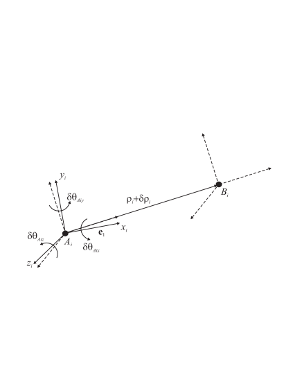
Figure 17: Variations in $A_{i}-B_{i}$ chain

According to Fig.17,

$${\bf b}_{i}-{\bf a}_{i}={\bf R}_{i}(\rho_{i}+\delta\rho_{i}){\bf e}_{1}+{\bf R}_{i}{\delta\theta}_{Ai}\times(\rho_{i}+\delta\rho_{i}){\bf e}_{1}$$ (35)

where $\rho_{i}$ is the displacement of the $i^{th}$ prismatic joint, $\delta\rho_{i}$ is its displacement error, $\delta\theta_{Ai}=\left[\begin{array}[]{ccc}\delta\theta_{Aix}&\delta\theta_{Aiy}&\delta\theta_{Aiz}\end{array}\right]^{T}$ is the angular variation of its direction, and

$${\bf e}_{1} = \left[\begin{array}[]{c}1\\ 0\\ 0\end{array}\right]$$ (39)

$${\bf e}_{2} = \left[\begin{array}[]{c}0\\ 0\\ 1\end{array}\right]$$ (43)

$$\xi(j) = \left\{\begin{array}[]{cc}1&\textrm{if }j=1\\ -1&\textrm{if }j=2\end{array}\right.$$ (46)

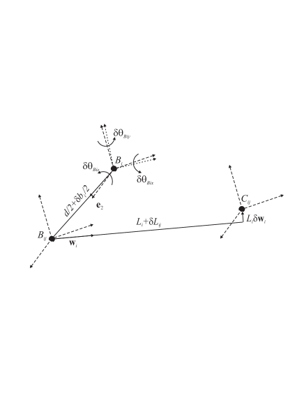
Figure 18: Variations in $B_{i}-B_{ij}-C_{ij}$ chain

According to Fig.18,

$${\bf b}_{ij}-{\bf b}_{i} = {\bf R}_{i}[{\bf I}_{3}+{\delta\theta}_{Ai}\times]\big{(}\xi(j)(d/2+\delta{b}_{i}/2)$$ (47)

$$[{\bf I}_{3}+\delta{\theta}_{Bi}\times]{\bf e}_{2}\big{)}$$

$${\bf c}_{ij}-{\bf b}_{ij} = L_{i}{\bf w}_{i}+\delta L_{ij}{\bf w}_{i}+L_{i}\delta{\bf w}_{i}$$ (48)

where $d$ is the nominal width of the parallelogram, $\delta{b}_{i}$ is the variation in the length of link $\overline{B_{i1}B_{i2}}$ and is supposed to be equally shared by each side of $B_{i}$. $\delta\theta_{Bi}=\left[\begin{array}[]{ccc}\delta\theta_{Bix}&\delta\theta_{Biy}&\delta\theta_{Biz}\end{array}\right]^{T}$ is the orientation error of link $\overline{B_{i1}B_{i2}}$ with respect to the direction of the $i^{th}$ prismatic joint, $L_{i}$ is the length of the $i^{th}$ parallelogram, $\delta L_{ij}$ is the variation in the length of link $\overline{B_{ij}C_{ij}}$, of which ${\bf w}_{i}$ is the direction, and $\delta{\bf w}_{i}$ is the variation in this direction, orthogonal to ${\bf w}_{i}$.

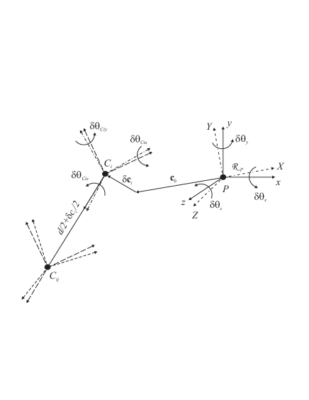
Figure 19: Variations in $C_{ij}-C_{i}-P$ chain

According to Fig.19,

$${\bf c}_{ij}-{\bf c}_{i} = {\bf R}_{i}[{\bf I}_{3}+\delta\theta\times]\big{(}\xi(j)(d/2+\delta{c}_{i}/2)$$ (49)

$$[{\bf I}_{3}+\delta{\theta}_{Ci}\times]{\bf e}_{2}\big{)}$$

$${\bf c}_{i}-{\bf p} = [{\bf I}_{3}+\delta\theta\times]{\bf R}_{i}({\bf c}_{0}+\delta{\bf c}_{i})$$ (50)

where $\delta{c}_{i}$ is the variation in the length of link $\overline{C_{i1}C_{i2}}$, which is supposed to be equally shared by each side of $C_{i}$. $\delta\theta_{Ci}=\left[\begin{array}[]{ccc}\delta\theta_{Cix}&\delta\theta_{Ciy}&\delta\theta_{Ciz}\end{array}\right]^{T}$ is the orientation error of link $\overline{C_{i1}C_{i2}}$ with respect to link $\overline{C_{i}P}$. ${\bf c}_{0}$ is the nominal position vector of $C_{i}$ with respect to end-effector $P$, expressed in ${\cal R}_{i}$, $\delta{\bf c}_{i}$ is the position error of $C_{i}$ expressed in ${\cal R}_{i}$, and $\delta\theta=\left[\begin{array}[]{ccc}\delta\theta_{x}&\delta\theta_{y}&\delta\theta_{z}\end{array}\right]^{T}$ is the orientation error of the end-effector, expressed in ${\cal R}_{b}$.

Implementing linearization of eqs.(25-49) and removing the components associated with the nominal constrained equation ${\bf p}_{0}={\bf R}_{i}({\bf a}_{0}+\rho_{i}{\bf e}_{1}-{\bf c}_{0})+L_{i}{\bf w}_{i}$, yields

$$\delta{\bf p} = {\bf p}-{\bf p}_{0}$$

$$= {\bf R}_{i}\big{(}\delta{\bf e}_{i}+\rho_{i}(\delta\theta_{Ai}\times{\bf e}_{1})+\xi(j)\ d/2\ (\delta\theta_{Ai}\times{\bf e}_{2})+$$

$$\xi(j)\ d/2\ (\delta\gamma_{i}\times{\bf e}_{2})+\xi(j)\ \delta{m_{i}}/2\ {\bf e}_{2}\big{)}+$$

$$\delta L_{ij}{\bf w}_{i}+L_{i}\delta{\bf w}_{i}-\delta\theta\times{\bf R}_{i}\big{(}{\bf c}_{0}+d/2\ \xi(j)\ {\bf e}_{2}\big{)}$$

where

$\delta{\bf p}$ is the position error of the end-effector of the manipulator.

$\delta{\bf e}_{i}=\delta{\bf a}_{i}+\delta{\rho}_{i}{\bf e}_{1}-\delta{\bf c}_{i}$ is the sum of the position errors of points $A_{i}$, $B_{i}$, and $C_{i}$ expressed in ${\cal R}_{i}$.

$\delta\gamma_{i}=\delta\theta_{Bi}-\delta\theta_{Ci}$ is the sum of the orientation errors of the $i^{th}$ parallelogram with respect to the $i^{th}$ prismatic joint and the end-effector.

$\delta{m_{i}}=\delta{b}_{i}-\delta{c}_{i}$ corresponds to the parallelism error of links $\overline{B_{i1}C_{i1}}$ and $\overline{B_{i2}C_{i2}}$, which is depicted by Fig.20.

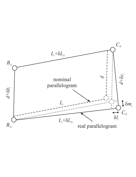
Figure 20: Variations in the $i^{th}$ parallelogram

Equation (3.2.1) shows the coupling of the position and orientation errors of the end-effector. Contrary to the orientation error, the position error can be compensated because the manipulator is a translational 3-DOF PKM. Thus, it is more important to minimize the geometrical variations, which are responsible for the orientation errors of the end-effector than the ones, which are responsible for its position errors.

The following equation is obtained by multiplying both sides of eq.(3.2.1) by ${\bf w}_{i}^{T}$ and utilizing the circularity of hybrid product.

$${\bf w}_{i}^{T}\delta{\bf p} = {\bf w}_{i}^{T}{\bf R}_{i}{\delta{\bf e}_{i}}+\rho_{i}({\bf R}_{i}{\bf e}_{1}\times{\bf w}_{i})^{T}{\bf R}_{i}\delta\theta_{Ai}+\xi(j)\ d/2$$

$$({\bf R}_{i}{\bf e}_{2}\times{\bf w}_{i})^{T}{\bf R}_{i}(\delta\theta_{Ai}+\delta\gamma_{i})+\xi(j)\ \delta{m_{i}}/2\ {\bf w}_{i}^{T}{\bf R}_{i}{\bf e}_{2}$$

$$+\delta L_{ij}-\big{(}{\bf R}_{i}({\bf c}_{0}+\xi(j)\ d/2\ {\bf e}_{2})\times{\bf w}_{i}\big{)}^{T}\delta\theta$$

Orientation Error Mapping Function: By substraction of eqs.(3.2.1) written for $j=1$ and $j=2$, and for the $i^{th}$ kinematic chain, a relation is obtained between the orientation error of the end-effector and the variations in design parameters, which is independent of the position error of the end-effector.

$$d({\bf R}_{i}{\bf e}_{2}\times{\bf w}_{i})^{T}\delta\theta=\delta l_{i}+d({\bf R}_{i}{\bf e}_{2}\times{\bf w}_{i})^{T}{\bf R}_{i}(\delta\theta_{Ai}+\delta\gamma_{i})+\delta{m_{i}}\ {\bf w}_{i}^{T}{\bf R}_{i}{\bf e}_{2}$$ (53)

where $\delta l_{i}=\delta L_{i1}-\delta L_{i2}$, the relative length error of links $\overline{B_{i1}C_{i1}}$ and $\overline{B_{i2}C_{i2}}$, depicts the parallelism error of links $\overline{B_{i1}B_{i2}}$ and $\overline{C_{i1}C_{i2}}$ as shown in Fig.20. Equation (53) can be written in matrix form:

$$\delta\theta={\bf J}_{\theta\theta}{\mbox{\boldmath${\epsilon}$\unboldmath}}_{\theta}$$ (54)

with

$${\bf J}_{\theta\theta} = {\bf D}^{-1}{\bf E}$$ (55)

$${\bf D} = d\left[\begin{array}[]{c}({\bf R}_{1}{\bf e}_{2}\times{\bf w}_{1})^{T}\\ ({\bf R}_{2}{\bf e}_{2}\times{\bf w}_{2})^{T}\\ ({\bf R}_{3}{\bf e}_{2}\times{\bf w}_{3})^{T}\end{array}\right]$$ (59)

$${\bf E} = \left[\begin{array}[]{ccc}{\bf E}_{1}&\cdots&\cdots\\ \cdots&{\bf E}_{2}&\cdots\\ \cdots&\cdots&{\bf E}_{3}\end{array}\right]$$ (63)

$${\bf E}_{i} = \left[\begin{array}[]{cccc}1&{\bf w}_{i}^{T}{\bf R}_{i}{\bf e}_{2}&d({\bf R}_{i}{\bf e}_{2}\times{\bf w}_{i})^{T}{\bf R}_{i}&d({\bf R}_{i}{\bf e}_{2}\times{\bf w}_{i})^{T}{\bf R}_{i}\end{array}\right]$$ (65)

$\delta\theta$ is the orientation error of the end-effector expressed in ${\cal R}_{b}$, and ${\mbox{\boldmath${\epsilon}$\unboldmath}}_{\theta}=({\mbox{\boldmath${\epsilon}$\unboldmath}}_{\theta 1}^{T},{\mbox{\boldmath${\epsilon}$\unboldmath}}_{\theta 2}^{T},{\mbox{\boldmath${\epsilon}$\unboldmath}}_{\theta 3}^{T})^{T}$ such that ${\mbox{\boldmath${\epsilon}$\unboldmath}}_{\theta i}=(\delta l_{i},\delta m_{i},\delta\theta_{Ai}^{T},\delta\gamma_{i}^{T})^{T}$. The determinant of ${\bf D}$ will be null if the normal vectors to the plans, which contain the three parallelograms respectively, are collinear, or if one parallelogram is flat. Here, this determinant is not null when $P$ covers $C_{u}$ because of the geometry of the manipulator. Therefore, ${\bf D}$ is nonsingular and its inverse ${\bf D}^{-1}$ exists.

As $({\bf R}_{i}{\bf e}_{2}\times{\bf w}_{i})^{T}\bot{\bf R}_{i}{\bf e}_{2}$, $\delta\theta_{Aiz}$ and $\delta\gamma_{iz}$, the third components of $\delta\theta_{Ai}$ and $\delta\gamma_{i}$ expressed in ${\cal R}_{i}$, have no effect on the orientation of the end-effector. Thus, matrix ${\bf J}_{\theta\theta}$ can be simplified by eliminating its columns associated with $\delta\theta_{Aiz}$ and $\delta\gamma_{iz}$, $i=1,2,3$. Finally, eighteen variations: $\delta l_{i}$, $\delta m_{i}$, $\delta\theta_{Aix}$, $\delta\theta_{Aiy}$, $\delta\gamma_{ix}$, $\delta\gamma_{iy}$, $i=1,2,3$, should be responsible for the orientation error of the end-effector.

Position Error Mapping Function: By addition of eqs.(3.2.1) written for $j=1$ and $j=2$, and for the $i^{th}$ kinematic chain, a relation is obtained between the position error of the end-effector and the variations in design parameters, which does not depend on $\delta\gamma_{i}$.

$${\bf w}_{i}^{T}\delta{\bf p}=\delta L_{i}+{\bf w}_{i}^{T}{\bf R}_{i}\delta{\bf e}_{i}+\rho_{i}({\bf R}_{i}{\bf e}_{1}\times{\bf w}_{i})^{T}{\bf R}_{i}\delta\theta_{Ai}-({\bf R}_{i}{\bf c}_{0}\times{\bf w}_{i})^{T}\delta\theta$$ (66)

Equation (66) can be written in matrix form:

$$\delta{\bf p}={\bf J}_{pp}{\mbox{\boldmath${\epsilon}$\unboldmath}}_{p}+{\bf J}_{p\theta}{\mbox{\boldmath${\epsilon}$\unboldmath}}_{\theta}=[{\bf J}_{pp}{\bf J}_{p\theta}]\left[\begin{array}[]{c}{\mbox{\boldmath${\epsilon}$\unboldmath}}_{p}\\ {\mbox{\boldmath${\epsilon}$\unboldmath}}_{\theta}\end{array}\right]$$ (67)

with

$${\bf J}_{pp} = {\bf F}^{-1}{\bf G}$$ (68)

$${\bf J}_{p\theta} = {\bf F}^{-1}{\bf H}{\bf J}_{\theta\theta}$$ (69)

$${\bf F} = [{\bf w}_{1}{\bf w}_{2}{\bf w}_{3}]^{T}$$ (70)

$${\bf G} = \mbox{diag}({\bf G}_{i})$$ (71)

$${\bf G}_{i} = \left[\begin{array}[]{ccc}1&{\bf w}_{i}^{T}{\bf R}_{i}&\rho_{i}({\bf R}_{i}{\bf e}_{1}\times{\bf w}_{i})^{T}{\bf R}_{i}\end{array}\right]$$ (73)

$${\bf H} = -\left[\begin{array}[]{ccc}{\bf R}_{1}{\bf c}_{0}\times{\bf w}_{1}&{\bf R}_{2}{\bf c}_{0}\times{\bf w}_{2}&{\bf R}_{3}{\bf c}_{0}\times{\bf w}_{3}\end{array}\right]$$ (75)

$${\mbox{\boldmath${\epsilon}$\unboldmath}}_{p} = ({\mbox{\boldmath${\epsilon}$\unboldmath}}_{p1}^{T},{\mbox{\boldmath${\epsilon}$\unboldmath}}_{p2}^{T},{\mbox{\boldmath${\epsilon}$\unboldmath}}_{p3}^{T})^{T}$$ (76)

$${\mbox{\boldmath${\epsilon}$\unboldmath}}_{pi} = (\delta L_{i},\delta{\bf e}_{i}^{T},\delta\theta_{Ai}^{T})^{T}$$ (77)

$\delta L_{i}=(\delta L_{i1}+\delta L_{i2})/2$ is the mean value of the variations in links $\overline{B_{i1}C_{i1}}$ and $\overline{B_{i2}C_{i2}}$, i.e.: the variation in the length of the $i^{th}$ parallelogram. ${\mbox{\boldmath${\epsilon}$\unboldmath}}_{p}$ is the set of the variations in design parameters, which should be responsible for the position errors of the end-effector, except the ones which should be responsible for its orientation errors, i.e.: ${\mbox{\boldmath${\epsilon}$\unboldmath}}_{\theta}$. ${\mbox{\boldmath${\epsilon}$\unboldmath}}_{p}$ is made up of three kinds of errors: the variation in the length of the $i^{th}$ parallelogram, i.e.: $\delta L_{i},i=1,2,3$, the position errors of points $A_{i}$, $B_{i}$, and $C_{i}$, i.e.: $\delta{\bf e}_{i},i=1,2,3$, and the orientation errors of the directions of the prismatic joints, i.e.: $\delta\theta_{Ai}$, $i=1,2,3$. Besides, ${\bf F}$ is nonsingular and its inverse ${\bf F}^{-1}$ exists because ${\bf F}$ corresponds to the Jacobian kinematic matrix of the manipulator, which is not singular when $P$ covers $C_{u}$, [9].

According to eq.(66) and as $({\bf R}_{i}{\bf e}_{1}\times{\bf w}_{i})^{T}\bot{\bf R}_{i}{\bf e}_{1}$, matrix ${\bf J}_{pp}$ can be simplified by eliminating its columns associated with $\delta\theta_{Aix},\ i=1,2,3$. Finally, thirty-three variations: $\delta L_{i}$, $\delta e_{ix}$, $\delta e_{iy}$, $\delta e_{iz}$, $\delta\theta_{Aix}$, $\delta\theta_{Aiy}$, $\delta\theta_{Aiz}$, $\delta l_{i}$, $\delta m_{i}$, $\delta\gamma_{ix}$, $\delta\gamma_{iy}$, $i=1,2,3$, should be responsible for the position error of the end-effector.

Rearranging matices ${\bf J}_{pp}$ and ${\bf J}_{p\theta}$, the position error of the end-effector can be expressed as:

$$\delta{\bf p}={\bf J}\ {\mbox{\boldmath${\epsilon}$\unboldmath}}_{q}=\left[\begin{array}[]{ccc}{\bf J}_{1}&{\bf J}_{2}&{\bf J}_{3}\end{array}\right]({\mbox{\boldmath${\epsilon}$\unboldmath}}_{q1}\ {\mbox{\boldmath${\epsilon}$\unboldmath}}_{q2}\ {\mbox{\boldmath${\epsilon}$\unboldmath}}_{q3})^{T}$$ (78)

with ${\mbox{\boldmath${\epsilon}$\unboldmath}}_{qi}=\big{(}\delta L_{i},\delta e_{ix},\delta e_{iy},\delta e_{iz},\delta\theta_{Aix},\delta\theta_{Aiy},\delta\theta_{Aiz},\delta l_{i},\delta m_{i},\delta\gamma_{ix},\delta\gamma_{iy}\big{)}$, and ${\bf J}\in{\mathbb{R}}^{3\times 33}$.

Sensitivity Indices: In order to investigate the influence of the design parameters errors on the position and the orientation of the end-effector, sensitivity indices are required. According to section 3.1.2, variations in the design parameters of the same type from one leg to the other have the same influence on the location of the end-effector. Thus, assuming that variations in the design parameters are independent, the sensitivity of the position of the end-effector to the variations in the $k^{th}$ design parameter responsible for its position error, i.e.: ${\epsilon}_{q(1,2,3)k}$, is called ${\mu}_{k}$ and is defined by eq.(79).

$${\mu}_{k}=\sqrt{\sum_{i=1}^{3}\sum_{m=1}^{3}J_{imk}^{2}}\ ,\ k=1,\cdots,11$$ (79)

Likewise, $\nu_{r}$ is a sensitivity index of the orientation of the end-effector to the variations in the $r^{th}$ design parameter responsible for its orientation error, i.e.: ${\epsilon}_{\theta(1,2,3)r}$. $\nu_{r}$ follows from eq.(54) and is defined by eq.(80).

$${\nu}_{r}=\arccos{\frac{\mathrm{tr}({\bf Q}_{r})-1}{2}}$$ (80)

where ${\bf Q}_{r}$ is the rotation matrix corresponding to the orientation error of the end-effector, and ${\nu}_{r}$ is a linear invariant: its global rotation [13].

$${\bf Q}_{r}=\left[\begin{array}[]{ccc}C_{{\nu}_{zr}}C_{{\nu}_{yr}}&\big{(}C_{{\nu}_{zr}}S_{{\nu}_{yr}}S_{{\nu}_{xr}}-S_{{\nu}_{zr}}C_{{\nu}_{xr}}\big{)}&\big{(}C_{{\nu}_{zr}}S_{{\nu}_{yr}}C_{{\nu}_{xr}}+S_{{\nu}_{zr}}S_{{\nu}_{xr}}\big{)}\\ S_{{\nu}_{zr}}C_{{\nu}_{yr}}&\big{(}S_{{\nu}_{zr}}S_{{\nu}_{yr}}S_{{\nu}_{xr}}+C_{{\nu}_{zr}}C_{{\nu}_{xr}}\big{)}&\big{(}S_{{\nu}_{zr}}S_{{\nu}_{yr}}C_{{\nu}_{xr}}-C_{{\nu}_{zr}}S_{{\nu}_{xr}}\big{)}\\ -S_{{\nu}_{yr}}&C_{{\nu}_{yr}}S_{{\nu}_{xr}}&C_{{\nu}_{yr}}C_{{\nu}_{xr}}\end{array}\right]$$ (81)

such that $C_{{\nu}_{xr}}=\cos{{\nu}_{xr}}$, $S_{{\nu}_{xr}}=\sin{{\nu}_{xr}}$, $C_{{\nu}_{yr}}=\cos{{\nu}_{yr}}$, $S_{{\nu}_{yr}}~{}=~{}\sin{{\nu}_{yr}}$, $C_{{\nu}_{zr}}=\cos{{\nu}_{zr}}$, $S_{{\nu}_{zr}}=\sin{{\nu}_{zr}}$, and

$${\nu}_{xr}=\sqrt{\sum_{j=0}^{2}J_{\theta\theta 1(6j+r)}^{2}}\ ,\ r=1,\cdots,6$$ (82)

$${\nu}_{yr}=\sqrt{\sum_{j=0}^{2}J_{\theta\theta 2(6j+r)}^{2}}\ ,\ r=1,\cdots,6$$ (83)

$${\nu}_{zr}=\sqrt{\sum_{j=0}^{2}J_{\theta\theta 3(6j+r)}^{2}}\ ,\ r=1,\cdots,6$$ (84)

Finally, ${\mu}_{k}$ can be employed as a sensitivity index of the position of the end-effector to the $k^{th}$ design parameter responsible for the position error. Likewise, ${\nu}_{r}$ can be employed as a sensitivity index of the orientation of the end-effector to the $r^{th}$ design parameter responsible for the orientation error. It is noteworthy that these sensitivity indices depend on the location of the end-effector.

3.2.2 Results of the Differential Vector Method

The sensitivity indices defined by eqs.(79) and (80) are used to evaluate the sensitivity of the position and orientation of the end-effector to variations in design parameters, particularly to variations in the parallelograms.

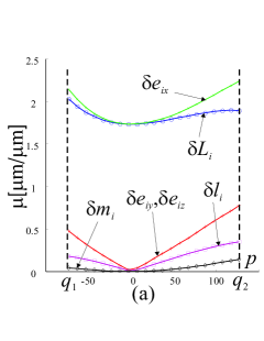
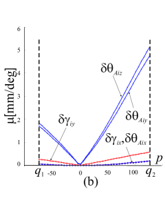
Figure 21: Sensitivity of the position of the end-effector along $Q_{1}Q_{2}$, (a): to dimensional variations, (b): to angular variations

Figures 21(a-b) depict the sensitivity of the position of the end-effector along the diagonal $Q_{1}Q_{2}$ of $C_{u}$, to dimensional variations and angular variations, respectively. According to Fig.21(a), the position of the end-effector is very sensitive to variations in the lengths of the parallelograms, $\delta L_{i}$, and to the position errors of points $A_{i}$, $B_{i}$, and $C_{i}$ along axis $x_{i}$ of ${\cal R}_{i}$, i.e: $\delta e_{ix}$. Conversely, the influence of $\delta l_{i}$ and $\delta m_{i}$, the parallelism errors of the parallelograms, is low and even negligible in the kinematic isotropic configuration. According to Fig.21(b), the orientation errors of the prismatic joints depicted by $\delta\theta_{Aiy}$ and $\delta\theta_{Aiz}$ are the most influential angular errors on the position of the end-effector. Besides, the position of the end-effector is not sensitive to angular variations in the isotropic configuration.

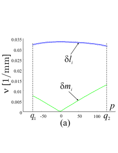
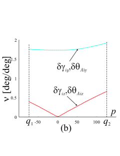
Figure 22: Sensitivity of the orientation of the end-effector along $Q_{1}Q_{2}$, (a): to dimensional variations, (b): to angular variations

Figures 22(a-b) depict the sensitivity of the orientation of the end effector, along $Q_{1}Q_{2}$, to dimensional and angular variations. According to Fig.22(a), $\delta l_{i}$ and $\delta m_{i}$ are the only dimensional variations, which are responsible for the orientation error of the end-effector. However, the influence of the parallelism error of the small sides of the parallelograms, depicted by $\delta l_{i}$, is more important than the one of the parallelism error of their long sides, depicted by $\delta m_{i}$.

According to figures 21 and 22, the sensitivity of the position and the orientation of the end-effector is generally null in the kinematic isotropic configuration ($p=0$), and is a maximum when the manipulator is close to a kinematic singular configuration, i.e.: $P\equiv Q_{2}$. Indeed, only two kinds of design parameters variations are responsible for the variations in the position of the end-effector in the isotropic configuration: $\delta L_{i}$ and $\delta e_{ix}$. Likewise, two kinds of variations are responsible for the variations in its orientation in this configuration: $\delta l_{i}$, the parallelism error of the small sides of the parallelograms, $\delta\theta_{Aiy}$ and $\delta\gamma_{iy}$. Moreover, the sensitivities of the pose (position and orientation) of the end-effector to these variations are a minimum in this configuration, except for $\delta l_{i}$. On the contrary, $Q_{2}$ configuration, i.e.: $P\equiv Q_{2}$, is the most sensitive configuration of the manipulator to variations in its design parameters. Indeed, as depicted by Figs.21 and 22, variations in the pose of the end-effector depend on all the design parameters variations and are a maximum in this configuration.

Moreover, figures 21 and 22 can be used to compute the variations in the position and the orientation of the end-effector with knowledge of the amount of variations in design parameters. For instance, let us assume that the parallelism error of the small sides of the parallelograms, $\delta l_{i}$, is equal to $10\mu$m. According to Fig.22(a), the position error of the end-effector will be equal about to $3\mu$m in $Q_{1}$ configuration ($P\equiv Q_{1}$). Likewise, according to Fig.21(b), if the orientation error of the direction of the $i^{th}$ prismatic joint round axis $y_{i}$ of ${\cal R}_{i}$ is equal to 1 degree, i.e.: $\delta\theta_{Aiy}=1$ degree, the position error of the end-effector will be equal about to 4.8 mm in $Q_{2}$ configuration.

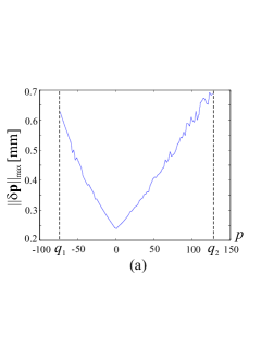
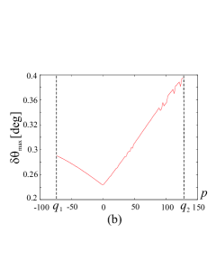
Figure 23: Maximum position (a) and orientation (b) errors of the end-effector along $Q_{1}Q_{2}$

Let us assume now that the length and angular tolerances are equal to 0.05 mm and 0.03 deg, respectively. Figure 23(a) shows the maximum position error of the end effector when it follows diagonal $Q_{1}Q_{2}$ of cube $C_{u}$. Likewise, Fig.23(b) shows the maximum orientation error of the end effector along $Q_{1}Q_{2}$. On both sides, the error is a minimum when the manipulator is in its kinematic isotropic configuration and is a maximum in $Q_{2}$ configuration. Besides, the maximum position and orientation errors of the end-effector are equal to 0.7 mm and 0.4 deg, respectively. These values correspond to the worst case scenario, which is unlikely.

Then, in order to take into account realistic machining tolerances, let us assume that the distribution of length and angular variations is normal.

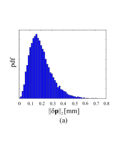
Figure 24: Repartition of the position error (a) and the orientation error (b) of the end-effector in $Q_{1}$ configuration

Figures 24 (a) and (b) illustrate the repartition of the position and the orientation errors of the end-effector in $Q_{1}$ configuration, respectively.

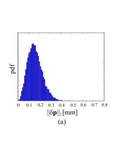
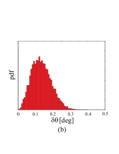
Figure 25: Repartition of the position error (a) and the orientation error (b) of the end-effector in the isotropic configuration

Figures 25 (a) and (b) illustrate the repartition of the position and the orientation errors of the end-effector in the kinematic isotropic configuration, respectively.

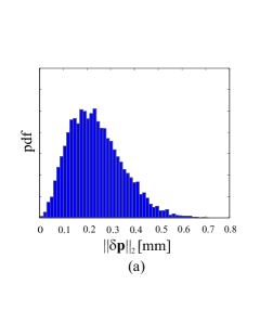
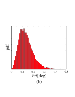
Figure 26: Repartition of the position error (a) and the orientation error (b) of the end-effector in $Q_{2}$ configuration

Figures 26 (a) and (b) illustrate the repartition of the position and the orientation errors of the end-effector in $Q_{2}$ configuration, respectively.

In Figures 24, 25, 26 (a) ((b), resp.) , the horizontal axis depicts the Euclidean norm of the position (orientation, resp.) error of the end-effector and the vertical axis depicts the corresponding probability density function (pdf). To plot these figures, we computed the position and orientation errors of the end-effector corresponding to more than three thousands sets of geometric variations following a normal distribution. For example, we can deduce from these calculations the probabilities to get a position error lower than 0.3 mm and an orientation error lower than 0.25 deg in $Q_{1}$, the isotropic, and $Q_{2}$ configurations.

	Configuration
	$Q_{1}$	Isotropic	$Q_{2}$
Prob($||\delta_{p}||_{2}\leq 0.3$ mm)	0.8468	0.9683	0.7276
Prob($\delta\theta\leq 0.25$ deg)	0.9691	0.9690	0.9453

Table 1: Probabilities to get a position error lower than 0.3 mm and an orientation error lower than 0.25 deg in $Q_{1}$, the isotropic, and $Q_{2}$ configurations

According to Table 1, the probability to get a position error lower than 0.3 mm is higher in the kinematic isotropic configuration than in $Q_{1}$ and $Q_{2}$ configurations. However, the probability to get an orientation error lower than 0.25 deg is the same in $Q_{1}$ and the isotropic configurations, but is lower in $Q_{2}$ configuration.

4 Conclusions

In this paper, two complementary methods were introduced to analyze the sensitivity of a three degree-of-freedom (DOF) translational Parallel Kinematic Machine (PKM) with orthogonal linear joints: the Orthoglide. Although these methods were applied to a particular PKM, they can be readily applied to 3-DOF Delta-Linear PKM such as ones with their linear joints parallel instead of orthogonal. Indeed, the input-output equations can be set in a very similar way since all Delta-linear PKM have identical leg kinematics, the only difference being in the closure equations [14].

On the one hand, a linkage kinematic analysis method was proposed to have a rough idea of the influence of the length variations of the manipulator on the location of its end-effector. On the other hand, a differential vector method was developed to study the influence of the length and angular variations in the parts of the manipulator on the position and orientation of its end-effector. This method has the advantage of taking into account the variations in the parallelograms.

According to the first method, variations in design parameters of the same type from one leg to another have the same effect on the end-effector. Besides, the position of the end-effector is very sensitive to variations in the lengths of parallelograms and prismatic joints. The second method shows that the parallelism errors of the bars of parallelograms are little influential on the position of the end-effector. Nevertheless, the orientation of the end-effector of the manipulator is more sensitive to the parallelism errors of the small sides of the parallelograms than to the ones of their long sides. Furthermore, it turns out that the sensitivity of the pose of the end-effector of the manipulator to geometric variations is a minimum in its kinematic isotropic configuration. On the contrary, this sensitivity approaches its maximum close to the kinematic singular configurations of the manipulator.

Therefore, these results should help the designer of the Orthoglide to synthesize its dimensional tolerances. Likewise, these methods can be applied to other Delta-Linear PKM with an aim of tolerance synthesis. Finally, the next steps in our research work are to compare the sensitivity of Delta-Linear PKM to variations in their geometric parameters, and to study the relation between the sensitivity and the stiffness of such manipulators.

This research, which is part of ROBEA-MP2 project, was supported by the CNRS (National Center of Scientific Research in France).

References

- [1] Wenger, P., Gosselin, C., and Maillé, B., 1999, A Comparative Study of Serial and Parallel Mechanism Topologies for Machine Tool, Int. Workshop on Parallel Kinematic Machines, Milan, Italie, pp. 23-35.
- [2] Wang, J., and Masory, O., 1993, On the accuracy of a Stewart platform - Part I, The effect of manufacturing tolerances., In: Proceedings of the IEEE International Conference on Robotics Automation, ICRA’93, Atlanta, USA, pp. 114-120.
- [3] Kim, H.S., and Choi, Y.J., 2000, The kinematic error bound analysis of the Stewart platform, Journal of Robotic Systems, 17, pp. 63-73.
- [4] Kim, H.S., and Tsai, L-W., 2003, Design optimization of a Cartesian parallel manipulator, ASME J. Mech. Des., 125, pp. 43-51.
- [5] Han, C., Kim, Ji., Kim, Jo., and Park F.C., 2002, Kinematic sensitivity analysis of the 3-UPU parallel mechanism, Mechanism and Machine Theory, 37, pp. 787-798.
- [6] Fan, K-C., Wang, H., Zhao, J-W., and Chang T-H., 2003, Sensitivity analysis of the 3-PRS parallel kinematic spindle platform of a serial-parallel machine tool, International Journal of Machine Tools & Manufacture, 43, pp. 1561-1569.
- [7] Verner, M., Fengfeng, X., and Mechefske, C., 2005, Optimal Calibration of Parallel Kinematic Machines, ASME J. Mech. Des., 127, pp. 62-69.
- [8] Caro, S., Bennis, F., and Wenger, P., 2005, Tolerance Synthesis of Mechanisms: A Robust Design Approach, ASME J. Mech. Des., 127, pp. 86-94.
- [9] Chablat, D., and Wenger, P., 2003, Architecture Optimization of a 3-DOF Parallel Mechanism for Machining Applications, The Orthoglide, IEEE Transactions On Robotics and Automation, 19, pp. 403-410.
- [10] Zanganeh, K.E., and Angeles, J., 1994, Kinematric isotropy and the optimum design of parallel manipulators, Int. J. of Rob. Research, 16, No.2, pp. 3-9.
- [11] Karouia, M., and Herve, J.M., 2002, A family of novel orientational 3-dof parallel robots, Proceedings of the CISM-IFToMM RoManSy Symposium, RoMansSy 14. (Edited by G. Bianchi, J.C. Guinot and Rzymkowski), Springer Verlag. Vienna, pp. 359-368.
- [12] Huang, T., Whitehouse, D.J., and Chetwynd, D.G., 2003, A Unified Error Model for Tolerance Design, Assembly and Error Compensation of 3-DOF Parallel Kinematic Machines with Parallelogram Sruts, Science in China Series E, ISSN:1006-9321, 20, 46, No.5, pp. 515-526.
- [13] Angeles, J., 2002, Fundamentals of Robotic Mechanical Systems, Springer-Verlag, New-York, edition.
- [14] Chablat, D., Wenger, P., Majou, F., and Merlet, J.P., 2004, An Interval Analysis Based Study for the Design and the Comparison of 3-DOF Parallel Kinematic Machines, International Journal of Robotics Research, 23, No.6, June, pp. 615-624.