Tidal waves as yrast states in transitional nuclei.

Abstract

The yrast states of transitional nuclei are described as quadrupole waves running over the nuclear surface, which we call tidal waves. In contrast to a rotor, which generates angular momentum by increasing the angular velocity at approximately constant deformation, a tidal wave generates angular momentum by increasing the deformation at approximately constant angular velocity. The properties of the tidal waves are calculated by means of the cranking model in a microscopic way. The calculated energies and E2 transition probabilities of the yrast states in the transitional nuclides with $Z$= 44, 46, 48 and $N=56,~{}58,~{}...,~{}66$ reproduce the experiment in detail. The nonlinear response of the nucleonic orbitals results in a strong coupling between shape and single particle degrees of freedom.

Most of the theoretical interpretation of the low-spin structure of nuclei in the transitional region between spherical and well deformed shape has been carried out in the framework of phenomenological models based on the Bohr - Hamiltonian[1, 2, 3] or using the algebraic IBM concept[4, 5, 6]. Although these studies account for many low-spin aspects of the collective quadrupole degree of freedom in an impressive way, the connection with the underlying microscopic structure has remained a challenge. On the other hand, the various versions of mean field theory are very successful in predicting shell closures, static deformations, and delineating the regions of spherical and deformed shapes (for recent reviews cf. e.g. [7, 8, 9]). Yet the large amplitude collective dynamics of transitional nuclei starting from the microscopic mean field remains a challenge to nuclear theory. At present there are two mature approaches of this type: the combination of mean field potential energy with cranking mass parameters (see review [10]) and the Generator Coordinate Method (see [11, 12] for recent development). Both approaches use the adiabatic approximation that the collective quadrupole excitations do not mix with the quasiparticle excitations, which is often not justified.

Figure 1: Potentials of a vibrator (V), soft rotor (R), and transitional nucleus (T).

In this Letter, we demonstrate that the yrast states of transitional nuclei have the very simple structure of a running surface wave (tidal wave), which permits us to calculate their properties microscopically by means of the cranked mean field theory without resorting to the adiabatic approximation. First we introduce the concept of tidal waves for the collective quadrupole vibrations of a classical droplet with irrotational flow, which is discussed in [1, 2]. Then we will extend it to the microscopic mean field theory and carry out calculations for a group of transitional nuclei around $A$=110.

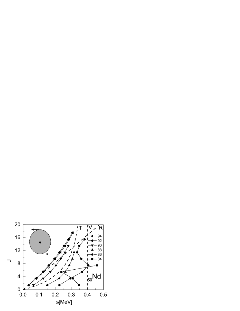
Figure 2: Angular momentum $J$ as function of the angular frequency $\omega$ (upper panel) and kinematic moment of inertia ${\cal J}$ as function of $J$ (lower panel) for the Nd-isotopes. The points correspond to $\omega(I)=(E(I)-E(I-2))/2$ and $J(I)=\sqrt{I(I-1)}/\omega(I)$, where $E(I)$ is the experimental yrast energy. The dashed lines show the cases discussed in the text.

The quadrupole displacement of the surface with respect to the sphere is $R(t)-R_{sph}=\sum_{\mu}\alpha_{\mu}(t)Y_{2\mu}(\vartheta,\varphi)$. The displacement is expressed by the familiar deformation parameters $\beta,\gamma$ and the vector $\vec{\phi}=\vec{n}\phi$ (rotation about the axis $\vec{n}$ by the angle $\phi$), which fixes the orientation of the quadrupole shape.

$$\alpha_{\mu}=U^{2}_{\mu 0}(\vec{\phi})\beta\cos{\gamma}+\left(U^{2}_{\mu 2}(\vec{\phi})+U^{2}_{\mu-2}(\vec{\phi})\right)\frac{\beta\sin{\gamma}}{\sqrt{2}}$$ (1)

(See [13] for the $U^{I}_{M,M^{\prime}}$ functions.) The kinetic energy is

$$2T=D(\dot{\beta}^{2}+\beta^{2}\dot{\gamma}^{2})+\sum_{i=1}^{3}\dot{\phi}^{2}_{i}{\cal J}_{i}$$ (2)

$${\cal J}_{i}=4D\beta^{2}\sin^{2}(\gamma-i\frac{2\pi}{3})$$ (3)

and the potential energy $V(\beta,\gamma)$ depends only on the deformation parameters. The equations of motion are derived from the Lagrangian $T-V$ in the standard way. The solution with maximal angular momentum $J$ in z-direction for given energy (yrast mode) is a wave that runs over the spherical surface with the constant angular velocity $\omega$. In the frame of reference rotating with the velocity $\omega$ the surface has a static deformation. The deformation parameters $\beta,\gamma$ are the equilibrium values at the minimum of the energy

$$E(\beta,\gamma)=\frac{J^{2}}{2{\cal J}(\beta,\gamma)}+V(\beta,\gamma),$$ (4)

$${\cal J}=4D\beta^{2}\sin^{2}(\gamma-\frac{2\pi}{3}),$$ (5)

where the angular momentum $J={\cal J}\omega$ and $\omega=dE/dJ$.

The location of the droplet surface in spherical coordinates is given by

$$R(t)=R_{o}[1+\sqrt{2}\beta\sin\gamma\cos(2\phi-2\omega t)Y_{22}(\vartheta,\varphi=0).$$ (6)

The inset of Fig. 2 illustrates this mode, which looks like the tidal waves on the oceans of our planet caused by the gravitational pull of moon and sun. In allusion, we suggest using this name for the running waves. Concerning the motion of the surface, it does not differ from rigid rotation. The difference between a rotor and a tidal wave is the way angular momentum is generated. The rigid rotor has a fixed deformation and a constant moment of inertia ${\cal J}$. The angular momentum $J={\cal J}\omega$ is generated by increasing the angular velocity $\omega$. The tidal wave runs with a fixed angular velocity $\omega$, while the angular momentum is gained by increasing the moment of inertia by changing $\beta,\gamma$. Of course, real nuclei lay between these idealized cases. Thus, we suggest the following classification: A rotor generates most of its angular momentum $J$ by increasing the angular frequency $\omega$, while the moment of inertia ${\cal J}$ does not change much. A tidal wave generates most of $J$ by increasing ${\cal J}$, while $\omega$ does not change much.

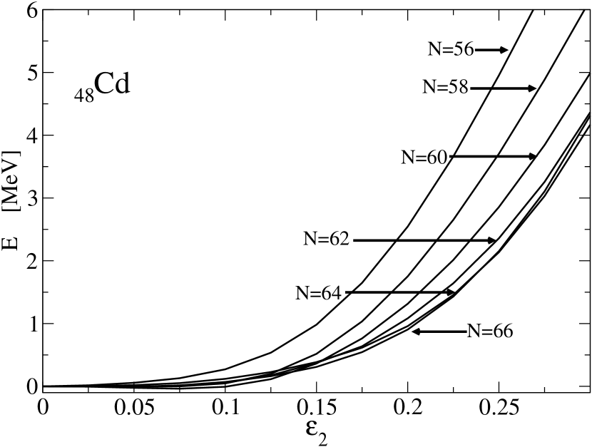
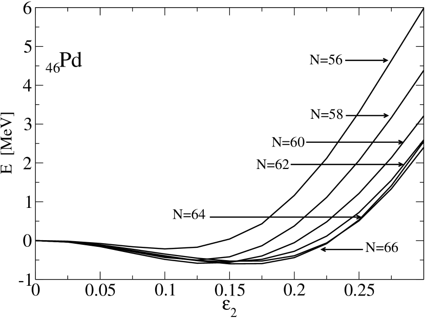
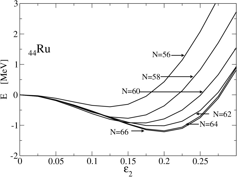
Figure 3: The ground state energies at $\gamma=5^{o}$.

Let us discuss some cases in more detail.
-Harmonic vibrator (V in Figs. 1,2):

$$V=\frac{C}{2}\beta^{2},$$ (7)

Minimizing the energy one finds

$$\gamma=\frac{\pi}{6},~{}\beta^{2}=\frac{J}{2\sqrt{DC}},~{}{\cal J}=4D\beta^{2}=\frac{2J}{\sqrt{DC}},$$ (8)

$$\omega=\frac{J}{{\cal J}}=\frac{1}{2}\sqrt{\frac{C}{D}},~{}E=\omega J=\Omega\frac{J}{2}=C\beta^{2}.$$ (9)

The wave travels with an angular velocity being one half of the oscillator frequency $\Omega$. The angular momentum is generated by only increasing the moment of inertia, which is a linear function of $J$. This is the ideal tidal wave. The solution with the same energy but $J=0$ is $R(t)=R_{0}(1+\beta\cos(\Omega t)Y_{20}(\vartheta))$, which is the familiar oscillation between prolate and oblate shapes.
-Rigid axial rotor (R in Fig. 2):

$$V=\frac{C\beta_{0}^{2}}{4}\left(-\left(\frac{\beta}{\beta_{0}}\right)^{2}+\frac{1}{2}\left(\frac{\beta}{\beta_{0}}\right)^{4}\right)+V_{g}\delta(\cos(3\gamma)-1)$$ (10)

The potential has a minimum at $\beta_{0}$, where $V\approx C(\beta-\beta_{0})^{2}/2$. Assuming $C$ being infinite large one finds

$$\gamma=-2\pi/3,\beta=\beta_{0},{\cal J}_{0}=3D\beta_{0}^{2}=const.$$ (11)

-The soft rotor: (R in Fig. 1)
With a finite $C$ the minimization gives

$$\beta=\beta_{0}(1+\frac{2J^{2}}{{\cal J}_{0}C\beta_{0}^{2}}+O(J^{4})),$$ (12)

$${\cal J}={\cal J}_{0}(1+\frac{8J^{2}}{{\cal J}_{0}C\beta_{0}^{2}}+O(J^{4})).$$ (13)

The moment of inertia is a slowly increasing quadratic function of $J$.
-Transitional nucleus (T in Figs. 1,2):
The yrast energies are well approximated by the expression suggested [14], which gives ($J=\sqrt{I(I+1)}$)

$$E(J)=\frac{J^{2}}{(2(\Theta_{0}+\Theta_{1}J)},~{}{\cal J}=\frac{(\Theta_{0}+\Theta_{1}J)^{2}}{(\Theta_{0}+\Theta_{1}J/2)}$$ (14)

As expected for a transitional nucleus, the angular momentum is gained by increasing both $\cal{J}$ and $\omega$. From a vibrational perspective, the increase of $\omega$ reflects the anharmonicities of the motion, from the rotational perspective, the increase of ${\cal J}$ reflects the softness of the rotor. Assuming the energies are derived from minimizing (4) and axial shape ($\gamma=0$) one finds

$$\frac{\beta(J)}{\beta_{0}}=\frac{\Theta_{0}+\Theta_{1}J}{\sqrt{B(\Theta_{0}+\Theta_{1}J/2)}},$$ (15)

$$V(J)=\frac{J^{2}(\Theta_{0}+\Theta_{1}J/2)}{(\Theta_{0}+\Theta_{1}J)^{2}},$$ (16)

which is a parametric form for $V(\beta/\beta_{0})$. It is displayed in Fig. 1 as T, which has a form intermediate the vibrator (V) and rotor (R). Using $Q_{t}=Q\beta/\beta_{0}$ for the transition quadrupole moment of E2-transitions, one may calculate its spin dependence by means of (15). Tab. 1 shows the case of ¹⁵⁴Gd, which has been classified as a transitional point nucleus [5, 16]. The parameters $\Theta_{0}=21.5$MeV^-1 and $\Theta_{1}=1.18$MeV^-1 place the nuclide slightly above the T -line in Fig. 2. The values for $Q_{t}$ are very similar to the ones of the X(5) limit given in [16], which is consistent with the the shape of the potential $V(\beta/\beta_{0})$. The increase of $Q_{t}$ is larger than that of the experimental values $Q_{t,exp}$, which points to degrees of freedom other than the quadrupole deformation contributing to the growth of ${\cal J}(I)$.

The transition between rotation and tidal waves is gradual. Let us classify the yrast mode of nuclei as an (anharmonic) tidal wave when most of the angular momentum is generated by the increase of the moment of inertia and as (soft) rotation when most of the angular momentum is generated by the increase of the angular velocity. Experimental functions $J(\omega)$ and ${\cal J}(J)$ can be derived from the level energies by the familiar procedure indicated in the caption of Fig. 2, which shows the Nd-isotopes. For the well deformed $N=94$ isotope, the increase of ${\cal J}$ remains moderate compared with ${\cal J}(0)$, and it grows approximately with $J^{2}$, which is characteristic for a rotor. The frequency $\omega$ starts with a small value and grows steadily. The isotopes with $N=84-88$ belong to the region of tidal waves. The frequency $\omega$ starts with a large value and stops growing, while ${\cal J}$ starts with a small value and increases substantially. As expected, $N=84$ comes closest to the spherical vibrator limit. The experimental functions $J(\omega)$ and ${\cal J}(J)$ become increasingly irregular when approaching the shell closure at $N=82$, which indicates that the the motion looses collectivity becoming progressively entangled with the single particle degrees of freedom. The limit of a good vibrator is not realized in nuclei. The isotop $N=90$ marks the border between a tidal wave and a soft rotor, which is in accordance with the onset of a substantial ground state deformation.

Table 1: Energies $E$ (in MeV) and transition quadrupole moments $Q$ (in eb) for ¹⁵⁴Gd. The subscript pm is used for the phenomenological model given by (14) and (15) and e for the experiment [15, 16]. The columns $\beta/\beta_{0}$ and $V$ display the deformation potential in parametric form.

$I$	$E_{e}$	$E_{pm}$	$\beta/\beta_{0}$	$V$	$Q_{t,e}$	$Q_{t,pm}$
0	0	0	0	0	-	-
2	0.123	0.123	1	0.11	6.2	6.2
4	0.371	0.374	1.07	0.33	6.52$\pm$0.06	6.64
6	0.717	0.720	1.14	0.62	6.42$\pm$0.10	7.05
8	1.144	1.142	1.20	0.95	6.60$\pm$0.16	7.45
10	1.637	1.623	1.26	1.31	-	7.84

The discussion of the liquid drop model for the quadrupole surface modes suggests that one may calculate the yrast states in a microscopic way by finding the selfconsistent mean field solution in a rotating frame of reference, i. e. one may use the cranking model for calculating the tidal wave modes in transitional and vibrational nuclei. In fact, [17] demonstrated that the RPA equations for harmonic quadrupole vibrations of nuclei with a spherical ground state are a solution to the selfconsistent cranking model if the deformation of the mean field is treated as a small perturbation. In this paper we solve numerically the cranking problem without the small deformation approximation, which allows us to describe the yrast states of all nuclei in the range between the harmonic vibrators and rigid rotors. Such microscopic approach takes into account not only the quadrupole shape degrees of freedom, as in the above discussed phenomenological model, but also the the quasiparticle degrees of freedom, which play an important role to be discussed below. Although we only study even-even nuclei in this Letter, we want to point out that the method can be applied to odd-A and odd-odd nuclei without any problems.

We use the Shell Correction version of the Tilted Axis Cranking model (SCTAC) in order to study the tidal waves in the nuclides with $Z=$44, 46, 48 and $N=$56, 58, 60, 62, 64, 66. The details and parameters of SCTAC are described in [18]. For the yrast states of even-even nuclei, the axis of rotation coincides with a principal axis (x). The condition $<J_{x}>=J=I$ is used to fix $\omega$, which is solved numerically for each point on a grid in the $\varepsilon_{2}-\gamma$ plane. In solving it is crucial to employ the diabatic tracing technique described in [18], which is illustrated in Fig. 4. The ground state (g-) configuration indicated by the full dots is followed through crossings of the h_11/2 routhians. The avoided crossings between the positve parity routhians around $\hbar\omega=0.53$ MeV are taken into account adiabatically: The occupation is kept on the lower of the two levels. The yrast states with high spin correspond to the s-configuration indicated by the open circles

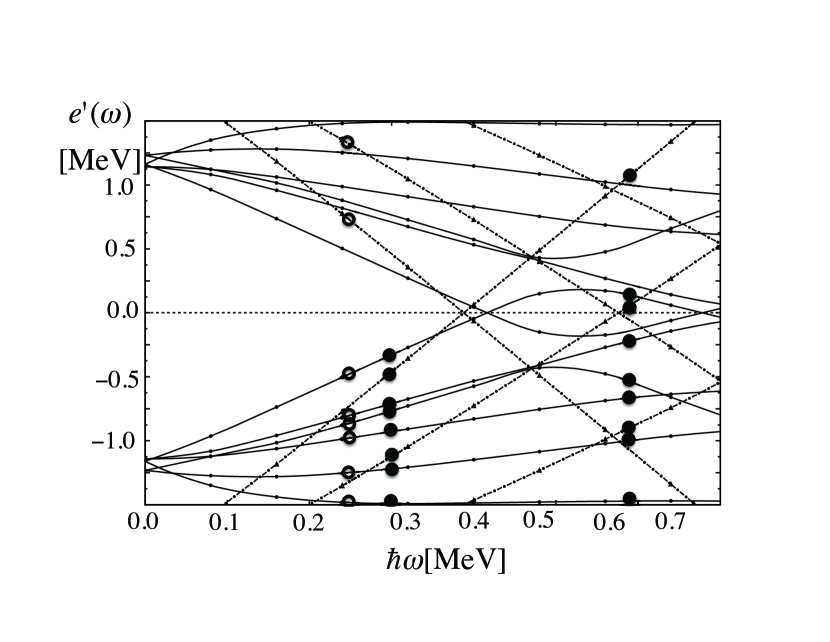
Figure 4: The Quasi Neutron Routhians for $N=62$ and $\varepsilon_{2}=0.13$, $\gamma=0$. Full lines: positive parity, dash dotted lines: negative parity (h_11/2). The full circles show the g-configuration, which corresponds to a tidal wave, the open circles show the s-configuration, which has the character of antimagnetic rotation.

The interpolated function $E(\varepsilon_{2},\gamma,J)$ is minimized with respect to deformation parameters for fixed angular momentum. The final value of $\omega(J)$ for the equilibrium deformation is found by interpolation between the values at the grid points. It is shown as the theoretical points in the Figure 5. It is noted, that the standard technique of finding the selfconsistent solutions by iteration at fixed $\omega$ becomes problematic for tidal waves close to the harmonic limit because the total Routhian is nearly deformation independent. The pairing parameters are kept fixed to $\Delta_{n}=\Delta_{p}=1.2$ MeV, and the chemical potentials are $\lambda$ adjusted to the particle numbers at $\omega=0$. The $B(E2,I->I-2)$ values are calculated for $J=I$ as described in [18] for $\theta=90^{o}$ and multiplied by $I(I-1)/(I-3/2)(I-1/2)$. The factor corrects for the low-spin deviation of the $B(E2)$ values from the high-spin limit used in the TAC code. It represents the Clebsh-Gordan coefficient appearing for axial $K=0$ bands [1], which is justified by the fact that for most nuclei $\gamma<10^{o}$. We slightly correct

$$J(\omega)=J_{SCTAC}(\omega)+100MeV^{-1}\varepsilon_{2}^{2}\sin^{2}(\gamma-\pi/3),$$ (17)

which adds less than 0.5 $\hbar$ to the angular momentum. About half of it takes into account the coupling between the oscillator shells and another half is expected to come from quadrupole pairing, both being neglected in SCTAC. The changes due to corrections are smaller than the radius of the open circles in Figs. 5 and 6.

The ground state energies are shown in Fig. 3. They are calculated using the modified oscillator potential with the parameters given in Ref. [18]. The tendency to deformation increases with the numbers of valence proton holes and valence neutron particles in the $Z=N=50$ shell. The $Z=48$ isotopes are spherical, becoming softer with increasing $N$. The $Z=44$ isotopes are slightly deformed, very soft, becoming less soft with $N$. The $Z=46$ isotopes are intermediate. Figs. 5 and 6 compare the calculated values of $J(\omega)$ and $B(E2,I->I-2)$ with experiment. The detailed agreement was achieved by adding to ground state deformation energies the small adjustment $k\varepsilon_{2}^{2}$ with $k=$8.5, 7.9, 8.5, 9.6, 11.9, 14.5 MeV for $N$= 56, 58, 60, 62, 64, 66, respectively, which makes the potentials slightly stiffer. The correction term is substantially smaller than the differences between deformation energies calculated from the various mean field theories used at present. Tab. 2 compares calculations with and without the correction term.

Table 2: Rotational frequencies in¹¹⁰Cd. The subscript o is used for the calculation without the correction of the ground state energies, the subscript c for the one with the correction, and the subscript e for the experiment. The calculated energy $E(0^{+}_{2})$=3.51 MeV, its experimental value 1.47 MeV. All energies are in MeV. Data from [15]

$I$	$\hbar\omega_{o}(0^{+}_{1})$	$\hbar\omega_{c}(0^{+}_{1})$	$\hbar\omega_{e}(0^{+}_{1})$	$\hbar\omega_{o}(0^{+}_{2})$	$\hbar\omega_{e}(0^{+}_{2})$
2	0.336	0.340	0.328	0.187	0.155
4	0.381	0.410	0.442	0.260	0.233
6	0.400	0.430	0.468	0.295	0.313
8	0.381	0.390	0.398
10	0.194	0.190	0.168
12	0.283	0.280	0.280

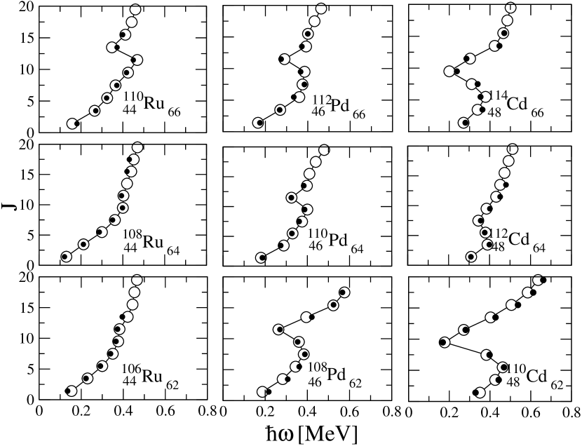
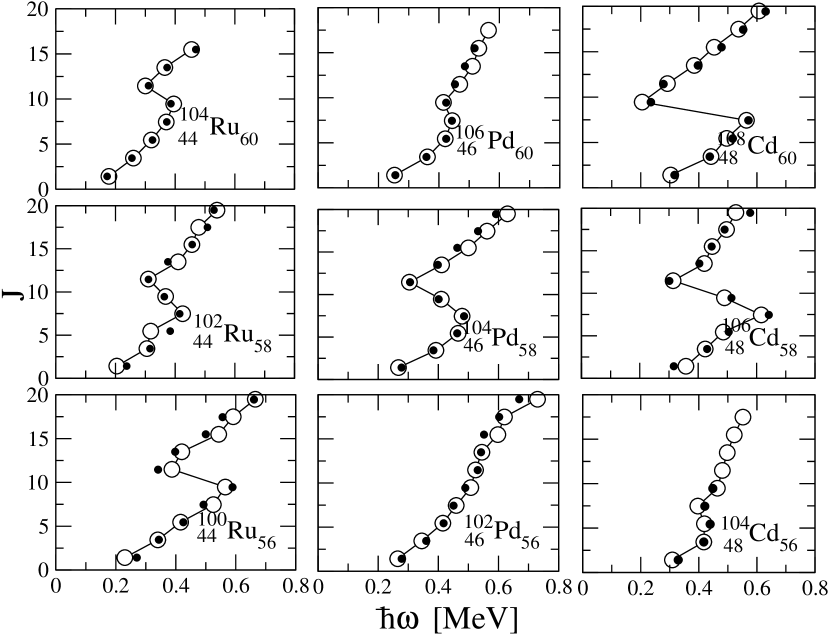
Figure 5: Angular momentum $J$ as function of the angular frequency $\omega$ in the mass 110 region. The quantities $J$ and $\omega$ are obtained as in Fig. 2 from the calculated or experimental yrast energies $E(I)$. Full symbols show the experiment, open the calculations. Data from [15].

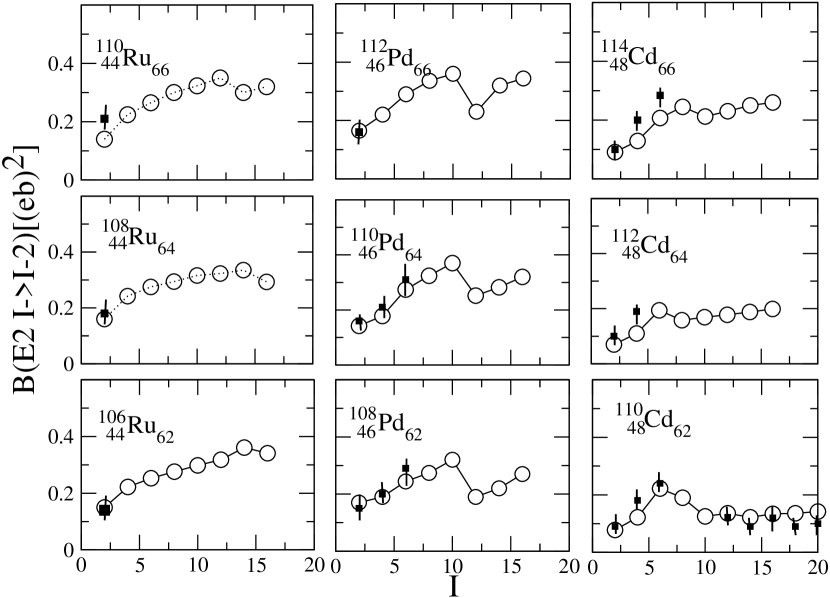
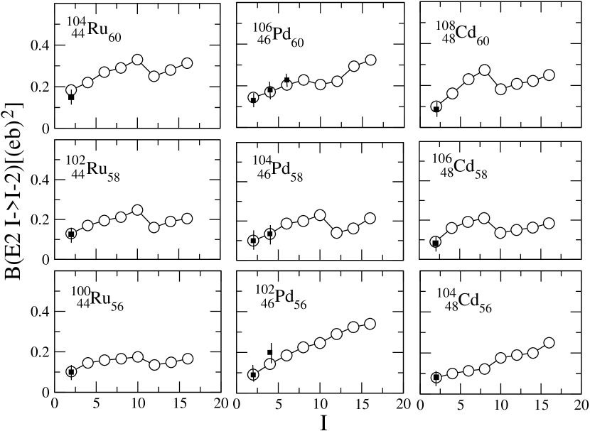
Figure 6: The $B(E2,I->I-2)$ values in the mass 110 region. Full symbols show the experiment, open the calculations. Data from [19, 15, 22, 20, 21, 23, 24, 25].

As seen in Fig. 6, for low-spin ($I\leq 6$) the tidal waves in Cd isotopes show the linear relation $B(E2)\propto J$ that is expected for vibrational nuclei. However, the energies deviate strongly from the vibrator limit. For Ru and Pd, the $B(E2)$ values start at larger values and increase less with $I$, such that they do not extrapolate to the origin. This reflects the transition to more rotational behavior, which becomes stronger with increasing $N$. The low-spin properties reflect the ground state deformation energies in Fig. 3.

At high spin, there is an irregularity in the $J(\omega)$ curves, which is caused by the rotational alignment of a pair of $h_{11/2}$ neutrons (change from the g-configuration to the s- configuration in Fig. 4). It is well known that the sharpness of the alignment depends sensitively on the position of the neutron chemical potential $\lambda_{n}$ relative to the $h_{11/2}$ levels [26], which causes the familiar oscillations between rapid alignment (back bending) and more gradual one (vertical section) with increasing $N$. The $h_{11/2}$ levels move with the changing deformation, and differences of the deformation are the reason why $J(\omega)$ sharply back bends in $Z=48,~{}N=62$ while it gradually grows in $Z=44,~{}N=62$. Also normal parity neutron orbitals contribute to the $J(\omega)$ in a non-linear way, in particular at the avoided crossings between them (around $\hbar\omega=$ 0.53 MeV in Fig. 4). For example, they are responsible that in ¹¹⁰Cd the point $I=8$ has a lower $\omega$ than the point $I=6$. The same is observed in ¹⁰⁸Cd [23] (not shown). The large frequency encountered at small deformation makes also other orbitals than the high-j intruders react in a non linear way to the inertial forces. For many nuclides the quasiparticle degrees cannot be treated in a perturbative way for $I\geq 6$, which means the separation of the collective quadrupole degrees of freedom becomes problematic. For the nuclei with the smallest numbers of valence particles and holes this entanglement of collective and single particle degrees appears already for $I=4$, which is reflected by the irregular curves $J(\omega)$ for $Z=48,~{}N=56$, and $Z=60,~{}N=84$ in Figs. 5, and 2, respectively.

As seen in Fig. 6, the aligned $h_{11/2}$ quasi neutrons stabilize the deformation at a smaller value than reached before, which is reflected by the decrease of the $B(E2)$ values. The deformation increases slower than before the alignment, which means that the motion becomes more rotational. In fact, it takes the character of Antimagnetic Rotation, discussed in [25]. In some cases, the alignment process is extended over several units of angular momentum, keeping $\omega$ nearly constant. This means the simple picture of tidal waves, as running at nearly constant angular velocity and gaining angular momentum by deforming does not account for the full complexity of real nuclei. Other degrees of freedom, in particular the single particle ones, may also provide angular momentum such that the rotational frequency remains constant.

¹⁰²Pd is a special case. The g- and s-configurations do not mix and are both observed up to $I=20$. Figs. 5 and 6 show only the g-sequence, which represents a tidal wave that gains angular momentum predominantly by increasing the deformation, as discussed above for the droplet model. Its amplitude at $I=16$ corresponds to eight stacked phonons! Only for $I>16$ the alignment of the positive parity neutrons (avoided crossing at $\hbar\omega\approx 0.53$ MeV in Fig. 4) becomes a comparable source of angular momentum.

Of course, our cranking approach also allows us to calculate rotational bands built on quasiparticle excitations. As an example, Tab. 2 contains the lowest two-quasiproton excitation across the $Z=50$ shell gap. The excited quasiprotons drive the nucleus to a substantial deformation, which, in contrast to one of the yrast tidal wave states, weakly increases with spin. The 0${}^{+}_{2}$ ”intruder state” has been assigned to this configuration, whose deformed shape coexists with the near spherical ground state shape [27]. The energies of the rotational band are well reproduced by the calculation, which however gives a too high energy of the $0^{+}_{2}$ state.

In conclusion, the yrast states of vibrational and transitional nuclei can be understood as tidal waves that run over the nuclear surface, which have a static deformation, the wave amplitude, in the frame of reference co-rotating with the wave. In contrast to rotors, most of the angular momentum is gained by an increase of the deformation while the angular velocity increases only weakly. Since tidal waves have a static deformation in the rotating frame, the rotating mean field approximation (Cranking model) provides a microscopic description. The yrast states of “spherical” or weakly deformed nuclei with $44\leq Z\leq 48,~{}56\leq N\leq 66$ were calculated up to spin 16. These microscopic calculations reproduce the energies and electromagnetic $E2$ transition probabilities in detail. The structure of the yrast states turns out to be complex. The shape degrees of freedom and the single particle degrees of freedom are intimately interwoven. The non-linear response to the inertial forces of the individual orbitals at the Fermi surface determines the way the angular momentum is generated. This lack of separation of the collective motion from the single particle becomes increasingly important with decreasing number of valence nucleons. It can set as low as $I=6$ already. Purely collective models like IBA [4] or the Dynamical Collective Model [2] miss this explicit coupling between single particle and collective freedoms.

Supported by the DoE Grant DE-FG02-95ER4093.

References

- [1] A. Bohr and B. R. Mottelson, Nuclear Structure, Vol. II (Benjamin, New York, 1975).
- [2] W. Greiner and J. Maruhn, Nuclear models (Springer, Berlin, 1996
- [3] M. Caprio, Phys. Lett. B 672, 396 (2009)
- [4] A. Arima and F. Iachello, The Interacting Boson Model (Cambridge University Press, Cambridge, U.K., 1987).
- [5] F. Iachello, Phys. Rev. Lett. 87, 052502 (2001).
- [6] E.A. McCutchan, R.F. Casten, Phys. Rev. C 74, 057302 (2006).
- [7] P. Möller et al., Phys. Rev. Lett. 97, 162502 (2006)
- [8] J.M. Pearson, S. Goriely, Nucl. Phys. A 777, 623 (2006).
- [9] M. V. Stoitsov, et al., Int. J. of Mass Spectrometry 251, 243 (2006).
- [10] L. Prochniak and S G Rohozinski, J. Phys. G 36, 123101(2009)
- [11] J. P. Delaroche, et al., Nucl. Phys. A 771, 103 (2006)
- [12] M. Bender and P. H. Heenen, Phys. Rev. C 78, 024309 (2008)
- [13] D. A. Varshalovich, et al., Quantum Theory of Angular Momentum (World Scientific, Singapore, 1988)
- [14] P. von Brentano et al., Phys. Rev. C 69, 044134 (2004)
- [15] ENSDF data bank, http://www.nndc.bnl.gov
- [16] D. Tonev et al., Phys. Rev C 69, 034334 (2004)
- [17] E.R. Marshalek, Phys. Rev. C 54 159 (1996).
- [18] S. Frauendorf, Nucl. Phys. A 677, 115 (2000).
- [19] S. Raman et al., Atomic D. and Nucl. D. Tab. 78, 1 (2001)
- [20] D. de Frenne, Nucl. Data Sheets 110, 1745 (2009)
- [21] D. de Frenne, E.Jacobs, Nucl. Data Sheets 89, 481 (2000).
- [22] L. E. Svensson, et al., Nucl. Phys. A 584, 574 (1995)
- [23] T. Thorslund et al. , Nucl. Phys. A 568, 306 (1994)
- [24] M. Piiparinen et al., Nucl. Phys. A 565, 671 (1993)
- [25] S. Frauendorf, Rev. Mod. Phys. 73, 463 (2001)
- [26] R. Bengtsson, et al., Phys. Lett. B 73, 259 (1978)
- [27] K. Heyde, et al. Phys. Rev. C 25, 3160 (1982)