Computed Coupling Efficiencies of Kolmogorov Phase Screens into Single-Mode Optical Fibers

Abstract

Coupling efficiencies of an electromagnetic field with a Kolmogorov phase statistics into a step-index fiber in its monomode regime of wavelengths are computed from the overlap integral between the phase screens and the far-field of the monomode at infrared wavelengths.

The phase screens are composed from Karhunen-Loève basis functions, optionally cutting off some of the eigenmodes of largest eigenvalue as if Adaptive Optics had corrected for some of the perturbations.

The examples are given for telescope diameters of 1 and 1.8 m, and Fried parameters of 10 and 20 cm. The wavelength of the stellar light is in the J, H, or K band of atmospheric transmission, where the fiber core diameter is tailored to move the cutoff wavelength of the monomode regime to the edges of these bands.

I Scope

One of the promises of monomode fiber optics is the removal of corrugations across pupil planes (“cleaning” of the beams) by symmetric weighting of the electric field across the pupil Mennesson et al. (2002); Wallner et al. (2002); Keen et al. (2001); Labadie et al. (2007). The transformation of phase screens is studied by computation of the overlap with the anticipated far-field distribution of the fiber optics of the detector system Shaklan and Roddier (1988). We demonstrate the negative impact of the growing number of speckles Roddier and Lena (1984) on the throughput of the spatial filter—represented by the fiber—as a function of telescope diameter. This combines essentially the work of Shellan Shellan (2004) —which describes the on-axis intensity after AO correction— with the specific spatial filtering of a fiber, which is roughly of Gaussian shape and therefore de-emphasizes the role of higher modes in Zernike expansions.

II Optical Setup and Model

II.1 Fibre Set

Step-index fibers are modeled with core radius $a$, refractive indices $n_{c}$ in the core and $n$ in the cladding, and the same numerical aperture

$$\alpha_{m}=1.4=\sqrt{n_{c}^{2}+n^{2}}$$ (1)

for all bands. The difference in $n_{c}-n$ is kept at 0.36 percent—copied from a specification of the Corning SMF-28e Photonic Fiber. This is rather hypothetical since we do not look at the absorption characteristics of materials in the infrared Laurent (2003); Dirnwöber (2005). The cutoff wavelengths $\lambda_{c}$ considered here are derived from the normalized frequency $v\approx 2.405$ Gloge (1971)

$$v=ak\alpha_{m},$$ (2)

where $k\equiv 2\pi/\lambda$ is the momentum number, which leads to the fiber specifications of Table 1.

Table 1: Choice of fiber geometries, cutoff wavelengths $\lambda_{c}$ and core radii $a$ in infrared bands.

band	$\lambda_{c}$ ($\mu$m)	$a$ ($\mu$m)	$n_{c}$	$n$
J	$1.13$	$3.089$	1.65437	$1.64843$
H	$1.36$	$3.718$	1.65437	$1.64843$
K	$1.87$	$5.112$	1.65437	$1.64843$

The two-dimensional distribution of the electric field at the fiber’s entrance is computed by matching the two Bessel Functions in the core and in the cladding at each individual wavelength $\lambda$ Gloge (1971); Stolen (1975). The electric field functions $f(\rho)$ depend only on the distance $\rho$ to the fiber axis (and parametrically on $\lambda$, $a$, $n_{c}$ and $n$), since no azimuthal dependence is left in the monomode regime. A numerical Hankel transform Agnesi et al. (1993); Ferrari et al. (1999); Magni et al. (1992); Markham and Conchello (2003); Perciante and Ferrari (2004); Stolen (1975); Cerjan (2007) transforms this into the far field $F({\bf r})$

$$F(r)\propto\int_{0}^{\infty}d\rho\,\rho f(\rho)J_{0}(\rho k\alpha)$$ (3)

in the pupil plane. (No Gaussian approximation to the far field Ruilier (1998); Wagner and Tomlinson (1982) is introduced.) The integration over the azimuthal angle over the fiber’s cut has already been performed in the Fraunhofer approximation, and has been condensed to the Bessel Function $J_{0}$. $r$ is the radial coordinate in the pupil plane, $\alpha\leq\alpha_{m}$ the angle from the fiber axis to this point in the pupil plane. The factor $\rho$ is the Jacobian from the introduction of circular coordinates in the plane of the fiber’s front face. The far field does not depend on the azimuthal angle $\theta$ in the pupil plane.

II.2 Phase Screens

The electric field in the exit pupil of the telescope is written as a two-dimensional phase screen over the radial coordinate $r$ and azimuthal coordinate $\theta$ as

$$E({\bf r})=e^{i\varphi(r,\theta)}.$$ (4)

Amplitude variations—scintillation as opposed to phase variations, or imaging characteristics Kouznetsov et al. (1997); Martin and Flatté (1988); Rodriguez-Gomez et al. (2005); Guyon (2002); Strömqvist Vetelino et al. (2007)—are not studied here, so the phases $\varphi({\bf r})$ are kept real-valued. Since we shall look only at coupling coefficients, the modulus of $E({\bf r})$ is arbitrarily normalized to unity.

The phase screens have been generated with a Kolmogorov spectrum by synthesizing Karhunen-Loève (KL) basis functions as described in the literature Fried (1978); Wang and Markey (1978); Roddier (1990); Mathar (2007):

$$\varphi(r)=\sum_{p,q}g_{p,q}K_{p}^{(q)}(r)\Theta_{q}(\theta).$$ (5)

We use normalized azimuthal basis functions

$$\Theta_{q}(\theta)\equiv\sqrt{\frac{\epsilon_{q}}{2\pi}}\times\left\{\begin{array}[]{c}\cos q\theta\\ \sin q\theta\end{array}\right.,$$ (6)

where

$$\epsilon_{q}\equiv\left\{\begin{array}[]{c@{,\quad}c}1&q=0\\ 2&q\geq 1\end{array}\right.$$ (7)

is Neumann’s factor. If the radial basis functions are normalized according to

$$\int_{0}^{D/2}rK_{p}^{(q)}(r)K_{p^{\prime}}^{(q^{\prime})}(r)dr=\delta_{pp^{\prime}},$$ (8)

the variance of the expansion coefficients is

$$\mathop{\mathrm{Var}}\nolimits g_{p,q}=D^{2}[D/r_{0}(\lambda)]^{5/3}{\cal B}_{p,q}^{2},$$ (9)

where ${\cal B}^{2}$ are the eigenvalues of a reduced KL equation Fried (1978). Note that there is some arbitrariness in distributing factors here: the factor $D^{2}$ in (9) might be absorbed in a renormalization of $K_{p}^{(q)}$, and the factor $\surd{\epsilon_{q}/(2\pi)}$ of (6) could also be dispersed over $K_{p}^{(q)}$ and/or $\cal B$.

The turbulent atmosphere is represented by a Kolmogorov power-law of the phase structure function—we do not discuss the validity of this ansatz from any fundamental or experimental point of view. The radial basis functions are generated numerically by solving the symmetrized integral equations for the eigen-modes $K_{p}^{(q)}$; Zernike polynomials Xia et al. (2007); Dai and Mahajan (2007); Sheppard et al. (2004); Comastri et al. (2007); ten Brummelaar (1996) or polynomials fits Dai (1995) have not been employed.

The Fried parameters $r_{0}$ that are quoted here are those implicitly measured at $0.5$ $\mu$m and were actually scaled with Fried (1978)

$$r_{0}(\lambda)=r_{0|0.5\mu\mathrm{m}}\left(\frac{\lambda}{0.5\mu\mathrm{m}}\right)^{6/5}$$ (10)

to the infrared wavelength $\lambda$ to generate the kernel of the KL integral equations. The radial functions $K_{p}^{(q)}$ are re-generated for each instance of the ratio $D/r_{0}(\lambda)$.

An Adaptive Optics (AO) correction parameter (degree) $c$ is introduced which assumes that some set of low-order basis functions with largest eigenvalues ${\cal B}_{p,q}$ is discarded while building the full phase screen. $c\geq 2$ means tip and tilt are removed from each individual phase screen, represented by the first line in (Wang and Markey, 1978, Table III); $c\geq 5$ means correction through refocus and astigmatism and removal of the first three lines in (Wang and Markey, 1978, Table III), and $c=14$ assumes correction of the modes of the first eight lines of (Wang and Markey, 1978, Table III). The calculations were done on a set of 75 basis functions, sufficiently large in comparison to these low-order corrections.

The survival of speckles is demonstrated by coupling 800 phase screens into a virtual photometric channel as if one would project a single telescope’s input, directly with the coupling lens onto the fiber head.

II.3 Coupling

The intensity coupling efficiency is computed from numerical evaluation of overlap integrals over the circular pupil Shaklan and Roddier (1988); Wagner and Tomlinson (1982),

$$A=\frac{|\int_{NA}E({\bf r})F(r)d^{2}r|^{2}}{\int_{NA}E^{*}({\bf r})E({\bf r})d^{2}r\,\int_{NA}F^{2}(r)d^{2}r}.$$ (11)

The phase screen samples are created by generation of independent phase screens from uncorrelated Gaussian random numbers for the expansion coefficients $g_{p,q}$; in that respect no time scale is needed to define the transit time from one sample of the Kolmogorov statistics to another Tubbs (2005); Kellerer and Tokovinin (2007); there is no such parameter as the wind velocity of Taylor screens Fusco et al. (2004).

Geometric imperfections like fiber misalignment Toyoshima (2006); Wagner and Tomlinson (1982) or splicing are not incorporated, nor Fresnel reflection losses at the fiber front end or a central obscuration (shadow of a secondary mirror) Hou et al. (2006).

For the Unit Telescopes of the Very Large Telescope Interferometer equipped with AO this has been studied in Felkel’s thesis Felkel (2005).

For weak turbulence, equation (4) can be expanded into its Taylor series $1+i\varphi-\varphi^{2}/2\cdots$. This decomposes the overlap integral in the numerator of (11) into a constant (which represents the limit of optimum coupling efficiency, $r_{0}\rightarrow\infty$), linear terms of azimuthal modes proportional to $\sin\theta$ or $\cos\theta$ which do not contribute because the integral vanishes, plus quadratic terms which are quadratic in $g_{p,q}{\cal B}^{2}_{p,q}$. The assessment of Ruilier and Fried that the energy coupling is represented by these terms remains basically correct, although the smearing with $F(r)$ diminishes the influence of terms of larger radial nodal numbers $p$.

III Phase Screen Statistics

Statistics over 800 phase screens have been compiled for sub-average ($r_{0}=10$ cm) and better-than-average ($r_{0}=20$ cm) seeing conditions Fusco et al. (2004); Percheron et al. (2006) for telescopes of $D=1$ m (Figures 1–6) and 1.8 m in diameter (Figures 7–12) at AO corrections levels of $c=2$, 5 and 14.

In each band, illumination by three different wavelengths $\lambda$ is studied, and the figures that follow are split into three panels. Standard diffraction theory shows how the blue components of spectra are enhanced for coupling into a waveguide of fixed geometry Pu (1993), but there is a counter-effect through the smoothing of the phase structure functions with (10). Here, the net effect is a higher coupling efficiency for the red end of the bands, in accordance with earlier results (Shaklan and Roddier, 1988, Fig. 1). This is not necessarily the full truth since the phase screen basis functions $K_{p}^{(q)}$ are calculated for each individual wavelength as a function of its phase structure function; as our model leaves a number $c$ of these aside, we are implicitly presuming that the AO performs on the same level at all wavelengths within a band, and this might not be realistic.

Tables 2 and 3 summarize the cumulative distribution function of each statistics by a triplet of values indicating the median (50 % percentile) and the offsets from there to the 84.1 % and 15.9 % percentiles, equivalent to providing error bars on a 1$\sigma$ level. The notation is $A_{50}+A_{84.1}-A_{15.9}$ where 50 percent of the coupling efficiencies are smaller than $A_{50}$, 15.9 percent are smaller than $A_{50}-A_{15.9}$, and 15.9 percent are larger than $A_{50}+A_{84.1}$.

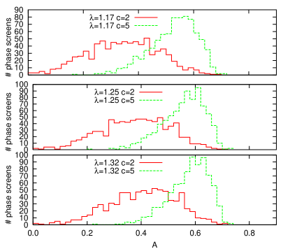
Figure 1: J-band. $D=1$ m. $r_{0}(500nm)=0.1$ m.

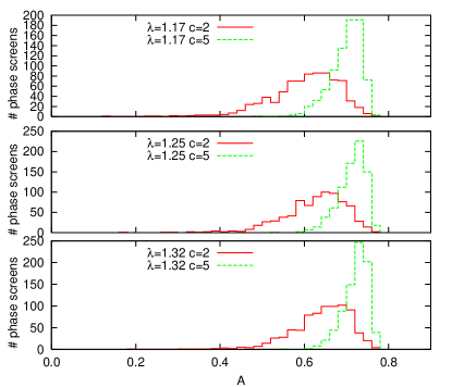
Figure 2: J-band. $D=1$ m. $r_{0}(500nm)=0.2$ m.

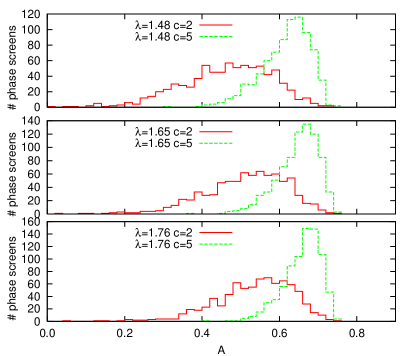
Figure 3: H-band. $D=1$ m. $r_{0}(500nm)=0.1$ m.

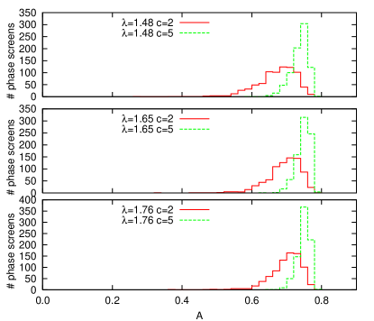
Figure 4: H-band. $D=1$ m. $r_{0}(500nm)=0.2$ m.

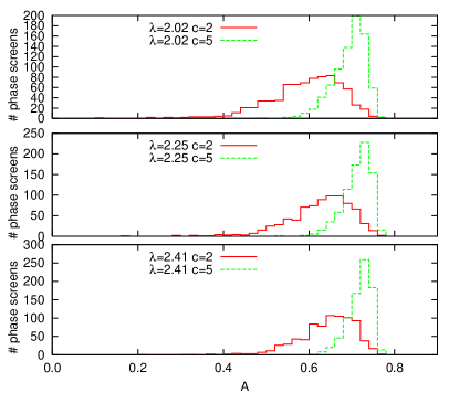
Figure 5: K-band. $D=1$ m. $r_{0}(500nm)=0.1$ m.

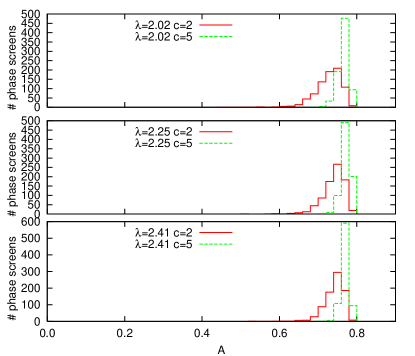
Figure 6: K-band. $D=1$ m. $r_{0}(500nm)=0.2$ m.

Table 2: Summary of percentiles of coupling efficiencies for a telescope diameter of $D=1$ m.

band	$r_{0}$ (500 nm)	Fig.	$\lambda$	$c$	${A_{50}}^{+A_{84.1}}_{-A_{15.9}}$
	(m)		($\mu$m)
J	0.1	1	1.17	2	$0.35^{+0.13}_{-0.14}$
J	0.1	1	1.17	5	$0.54^{+0.07}_{-0.10}$
J	0.1	1	1.25	2	$0.39^{+0.13}_{-0.14}$
J	0.1	1	1.25	5	$0.57^{+0.06}_{-0.09}$
J	0.1	1	1.32	2	$0.42^{+0.12}_{-0.14}$
J	0.1	1	1.32	5	$0.59^{+0.06}_{-0.09}$
J	0.2	2	1.17	2	$0.61^{+0.07}_{-0.10}$
J	0.2	2	1.17	5	$0.71^{+0.03}_{-0.04}$
J	0.2	2	1.25	2	$0.64^{+0.06}_{-0.09}$
J	0.2	2	1.25	5	$0.72^{+0.02}_{-0.04}$
J	0.2	2	1.32	2	$0.65^{+0.05}_{-0.08}$
J	0.2	2	1.32	5	$0.73^{+0.02}_{-0.03}$
H	0.1	3	1.48	2	$0.48^{+0.11}_{-0.14}$
H	0.1	3	1.48	5	$0.63^{+0.05}_{-0.07}$
H	0.1	3	1.65	2	$0.53^{+0.09}_{-0.12}$
H	0.1	3	1.65	5	$0.66^{+0.04}_{-0.06}$
H	0.1	3	1.76	2	$0.55^{+0.08}_{-0.12}$
H	0.1	3	1.76	5	$0.67^{+0.04}_{-0.06}$
H	0.2	4	1.48	2	$0.68^{+0.04}_{-0.07}$
H	0.2	4	1.48	5	$0.74^{+0.02}_{-0.03}$
H	0.2	4	1.65	2	$0.70^{+0.04}_{-0.06}$
H	0.2	4	1.65	5	$0.75^{+0.01}_{-0.02}$
H	0.2	4	1.76	2	$0.71^{+0.03}_{-0.05}$
H	0.2	4	1.76	5	$0.75^{+0.01}_{-0.02}$
K	0.1	5	2.02	2	$0.61^{+0.07}_{-0.10}$
K	0.1	5	2.02	5	$0.70^{+0.03}_{-0.05}$
K	0.1	5	2.25	2	$0.64^{+0.06}_{-0.09}$
K	0.1	5	2.25	5	$0.72^{+0.02}_{-0.04}$
K	0.1	5	2.41	2	$0.65^{+0.05}_{-0.08}$
K	0.1	5	2.41	5	$0.72^{+0.02}_{-0.03}$
K	0.2	6	2.02	2	$0.73^{+0.03}_{-0.04}$
K	0.2	6	2.02	5	$0.77^{+0.01}_{-0.02}$
K	0.2	6	2.25	2	$0.74^{+0.02}_{-0.03}$
K	0.2	6	2.25	5	$0.77^{+0.01}_{-0.01}$
K	0.2	6	2.41	2	$0.75^{+0.02}_{-0.03}$
K	0.2	6	2.41	5	$0.77^{+0.01}_{-0.01}$

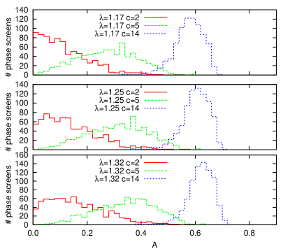
Figure 7: J-band. $D=1.8$ m. $r_{0}(500nm)=0.1$ m.

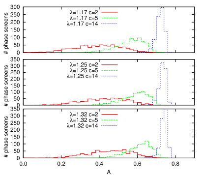
Figure 8: J-band. $D=1.8$ m. $r_{0}(500nm)=0.2$ m.

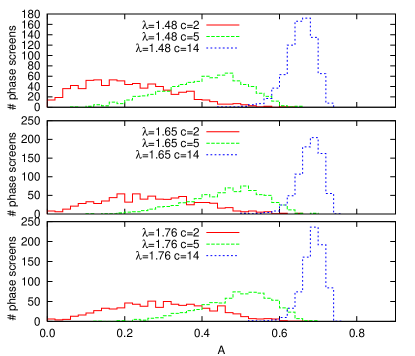
Figure 9: H-band. $D=1.8$ m. $r_{0}(500nm)=0.1$ m.

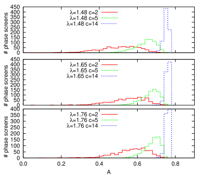
Figure 10: H-band. $D=1.8$ m. $r_{0}(500nm)=0.2$ m.

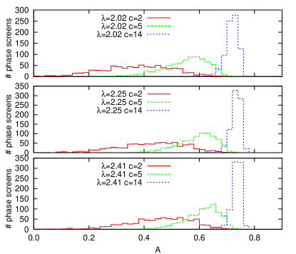
Figure 11: K-band. $D=1.8$ m. $r_{0}(500nm)=0.1$ m.

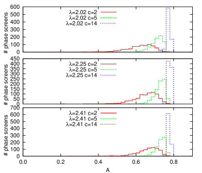
Figure 12: K-band. $D=1.8$ m. $r_{0}(500nm)=0.2$ m.

Table 3: Summary of percentiles of coupling efficiencies, $D=1.8$ m.

band	$r_{0}$ (500 nm)	Fig.	$\lambda$	$c$	${A_{50}}^{+A_{84.1}}_{-A_{15.9}}$
	(m)		($\mu$m)
J	0.1	7	1.17	5	$0.28^{+0.11}_{-0.12}$
J	0.1	7	1.17	14	$0.58^{+0.05}_{-0.06}$
J	0.1	7	1.25	5	$0.32^{+0.11}_{-0.12}$
J	0.1	7	1.25	14	$0.61^{+0.05}_{-0.05}$
J	0.1	7	1.32	5	$0.35^{+0.11}_{-0.12}$
J	0.1	7	1.32	14	$0.62^{+0.04}_{-0.05}$
J	0.2	8	1.17	5	$0.57^{+0.06}_{-0.09}$
J	0.2	8	1.17	14	$0.72^{+0.02}_{-0.02}$
J	0.2	8	1.25	5	$0.60^{+0.06}_{-0.08}$
J	0.2	8	1.25	14	$0.73^{+0.02}_{-0.02}$
J	0.2	8	1.32	5	$0.62^{+0.05}_{-0.08}$
J	0.2	8	1.32	14	$0.74^{+0.01}_{-0.02}$
H	0.1	9	1.48	5	$0.41^{+0.10}_{-0.12}$
H	0.1	9	1.48	14	$0.66^{+0.03}_{-0.04}$
H	0.1	9	1.65	5	$0.47^{+0.09}_{-0.11}$
H	0.1	9	1.65	14	$0.68^{+0.03}_{-0.03}$
H	0.1	9	1.76	5	$0.50^{+0.08}_{-0.11}$
H	0.1	9	1.76	14	$0.69^{+0.03}_{-0.03}$
H	0.2	10	1.48	5	$0.65^{+0.04}_{-0.06}$
H	0.2	10	1.48	14	$0.75^{+0.01}_{-0.01}$
H	0.2	10	1.65	5	$0.68^{+0.04}_{-0.05}$
H	0.2	10	1.65	14	$0.76^{+0.01}_{-0.01}$
H	0.2	10	1.76	5	$0.69^{+0.03}_{-0.05}$
H	0.2	10	1.76	14	$0.76^{+0.01}_{-0.01}$
K	0.1	11	2.02	5	$0.56^{+0.07}_{-0.09}$
K	0.1	11	2.02	14	$0.72^{+0.02}_{-0.02}$
K	0.1	11	2.25	5	$0.60^{+0.06}_{-0.08}$
K	0.1	11	2.25	14	$0.73^{+0.02}_{-0.02}$
K	0.1	11	2.41	5	$0.62^{+0.05}_{-0.07}$
K	0.1	11	2.41	14	$0.74^{+0.01}_{-0.02}$
K	0.2	12	2.02	5	$0.72^{+0.03}_{-0.04}$
K	0.2	12	2.02	14	$0.77^{+0.01}_{-0.01}$
K	0.2	12	2.25	5	$0.73^{+0.02}_{-0.03}$
K	0.2	12	2.25	14	$0.78^{+0.01}_{-0.01}$
K	0.2	12	2.41	5	$0.74^{+0.02}_{-0.03}$
K	0.2	12	2.41	14	$0.78^{+0.00}_{-0.01}$

IV Summary

A compact view on the median coupling efficiencies of these two tables is given in Figure 13. The values on the curve with the red crosses, $c=2$, are slightly more optimistic than those of Shaklan-Roddier (Shaklan and Roddier, 1988, Fig. 2) which one may attribute to underestimation of efficiencies by the Gaussian approximation.

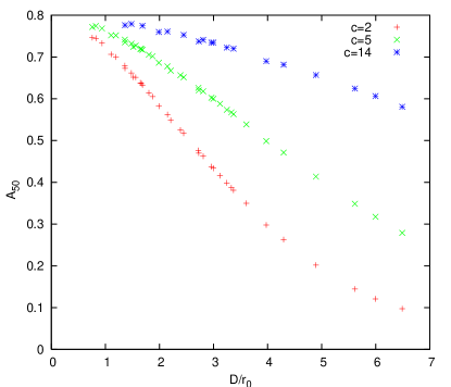
Figure 13: Coupling efficiencies (medians) sorted with respect to $D/r_{0}(\lambda)$ and the level of AO correction. Each curve of Figures 1–12 is represented by one marker of its associated color.

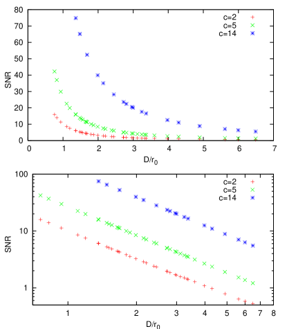
Figure 14: The signal-to-noise ratio represents the median coupling efficiency divided by the statistical width of the distributions (1$\sigma$ error bars). Both plots represent the same data set, one marker for each of the curves in Figures 1–12, the upper on linear and the lower on logarithmic axis scales.

By dividing the median through the noise introduced by the Kolmogorov fluctuation in the phases, we obtain $A_{50}/(A_{84.1}-A_{15.9})$ as a signal-to-noise ratio (SNR) for each combination of fiber geometry, wavelength, telescope diameter, Fried parameter and AO correction. Figure 14 shows these twice. The aim of the doubly logarithmic representation is to demonstrate that the SNR can be well fitted by a power law $\propto(D/r_{0})^{-5/3}$ with a prefactor depending only on the AO correction level $c$ Ruilier and Cassaing (2001). This is not unexpected because this power has been an input to equation (9), and for a pinhole type of spatial filter this remains essentially unharmed as reasoned in Sect. II.3 Noll (1976).

Reduced coupling efficiencies as a function of the number of speckles and degree of AO correction have been well reported by Shaklan and Roddier. We have illustrated that in addition this reduction in photometric signals is accompanied by wider variances of the expected coupling efficiency, which leads to the need of longer integration times during observations.

References

- Agnesi et al. (1993) Agnesi, A., G. C. Reali, G. Patrini, and A. Tomaselli, 1993, J. Opt. Soc. Am. A 10(9), 1872.
- Cerjan (2007) Cerjan, C., 2007, J. Opt. Soc. Am. A 24(6), 1609.
- Comastri et al. (2007) Comastri, S. A., L. I. Perez, G. D. Pérez, G. Martin, and K. Bastida, 2007, J. Opt. A: Pure Appl. Opt. 9(3), 209.
- Dai (1995) Dai, G.-m., 1995, J. Opt. Soc. Am. A 12(10), 2182.
- Dai and Mahajan (2007) Dai, G.-m., and V. N. Mahajan, 2007, J. Opt. Soc. Am. A 24(1), 139.
- Dirnwöber (2005) Dirnwöber, M., 2005, Characterization of Optial Fibers in the Mid-Infrared, Master’s thesis, Technische Universität Wien.
- Felkel (2005) Felkel, R., 2005, Kompensation der atmosphärischen Turbulenz in einer optischen Antennengruppe, Master’s thesis, Technische Universität Wien.
- Ferrari et al. (1999) Ferrari, J. A., D. Perciante, and A. Dubra, 1999, J. Opt. Soc. Am. A 16(10), 2581.
- Fried (1978) Fried, D. L., 1978, J. Opt. Soc. Am. 68(12), 1651.
- Fusco et al. (2004) Fusco, T., G. Rousset, D. Rabaud, E. Gendron, D. Mouillet, F. Lacombe, G. Zins, P.-Y. Madec, A.-M. Lagrange, J. Charton, D. Rouan, N. Hubin, et al., 2004, J. Opt. A 6(6), 585.
- Gloge (1971) Gloge, D., 1971, Appl. Opt. 10(10), 2252.
- Guyon (2002) Guyon, O., 2002, Astron. Astrophys. 387(1), 366.
- Hou et al. (2006) Hou, X., F. Wu, L. Yang, and Q. Chen, 2006, Appl. Opt. 45(35), 8893.
- Keen et al. (2001) Keen, J. W., D. F. Buscher, and P. J. Warner, 2001, Month. Not. Roy. Astron. Soc. 326(4), 1381.
- Kellerer and Tokovinin (2007) Kellerer, A., and A. Tokovinin, 2007, Astron. Astroph. 461(2), 775.
- Kouznetsov et al. (1997) Kouznetsov, D., V. V. Voitsekhovich, and R. Ortega-Martinez, 1997, Appl. Opt. 36(2), 464.
- Labadie et al. (2007) Labadie, L., E. L. Coarer, R. Maurand, P. Labeye, P. Kern, B. Arezki, and J.-E. Broquin, 2007, Astron. Astrophys. 471(1), 355.
- Laurent (2003) Laurent, E., 2003, Premiers développements de l’optique intégrée planaire monomode pour les longueurs d’onde entre 2 et 20 micromètres. Applications à l’interférométrie stellaire., Ph.D. thesis, L’Institut de Microélectronique, Électromagnétisme et Photonique, Grenoble.
- Magni et al. (1992) Magni, V., G. Cerullo, and S. De Silvestri, 1992, J. Opt. Soc. Am. A 9(11), 2031.
- Markham and Conchello (2003) Markham, J., and J.-A. Conchello, 2003, J. Opt. Soc. Am. A 20(4), 621.
- Martin and Flatté (1988) Martin, J. M., and S. M. Flatté, 1988, Appl. Opt. 27(11), 2111.
- Mathar (2007) Mathar, R. J., 2007, arXiv:astro-ph/0705.1700 .
- Mennesson et al. (2002) Mennesson, B., M. Ollivier, and C. Ruilier, 2002, J. Opt. Soc. Am. A 19(3), 596.
- Noll (1976) Noll, R. J., 1976, J. Opt. Soc. Am. 66(3), 207.
- Percheron et al. (2006) Percheron, I., M. Wittkowski, R. Donaldson, E. Fedrigo, C. Lidman, S. Morel, F. Rantakyro, M. Schöller, and A. Wallander, 2006, in Advances in Stellar Interferometry, edited by J. D. Monnier, M. Schöller, and W. Danchi (Int. Soc. Optical Engineering), volume 6268, pp. 1268–1275.
- Perciante and Ferrari (2004) Perciante, C. D., and J. A. Ferrari, 2004, J. Opt. Soc. Am. A 21(9), 1811.
- Pu (1993) Pu, J., 1993, J. Optics (Paris) 24(3), 141.
- Roddier and Lena (1984) Roddier, F., and P. Lena, 1984, J. Optics (Paris) 15(6), 363.
- Roddier (1990) Roddier, N., 1990, Opt. Eng. 29(10), 1174.
- Rodriguez-Gomez et al. (2005) Rodriguez-Gomez, A., F. Dios, J. A. Rubio, and A. Comeron, 2005, Appl. Opt. 44(21), 4574.
- Ruilier (1998) Ruilier, C., 1998, in Astronomical Interferometry, edited by R. D. Reasenberg (Int. Soc. Optical Engineering), volume 3350 of Proc. SPIE, pp. 319–329.
- Ruilier and Cassaing (2001) Ruilier, C., and F. Cassaing, 2001, J. Opt. Soc. Am. A 18(1), 143.
- Shaklan and Roddier (1988) Shaklan, S. B., and F. Roddier, 1988, Appl. Opt. 27(11), 2334.
- Shellan (2004) Shellan, J. B., 2004, J. Opt. Soc. Am. A 21(8), 1445.
- Sheppard et al. (2004) Sheppard, C. J. R., S. Campbell, and M. D. Hirschhorn, 2004, Appl. Opt. 43(20), 3963.
- Stolen (1975) Stolen, R. H., 1975, Appl. Opt. 14(7), 1533.
- Strömqvist Vetelino et al. (2007) Strömqvist Vetelino, F., C. Young, L. Andrews, and J. Recolons, 2007, Appl. Opt. 46(11), 2099.
- ten Brummelaar (1996) ten Brummelaar, T. A., 1996, Opt. Commun. 132(2), 329.
- Toyoshima (2006) Toyoshima, M., 2006, J. Opt. Soc. Am. A 23(9), 2246.
- Tubbs (2005) Tubbs, R. N., 2005, Appl. Opt. 44(29), 6253.
- Wagner and Tomlinson (1982) Wagner, R. E., and W. J. Tomlinson, 1982, Appl. Opt. 21(15), 2671.
- Wallner et al. (2002) Wallner, O., W. R. Leeb, and P. J. Winzer, 2002, J. Opt. Soc. Am. A 19(12), 2445.
- Wang and Markey (1978) Wang, J. Y., and J. K. Markey, 1978, J. Opt. Soc. Am. 68(1), 78.
- Xia et al. (2007) Xia, T., H. Zhu, H. Shu, P. Haigron, and L. Luo, 2007, J. Opt. Soc. Am. A 24(1), 50.