Vortices on a superconducting nanoshell: phase diagram and dynamics

Abstract

In superconductors, the search for special vortex states such as giant vortices focuses on laterally confined or nanopatterned thin superconducting films, disks, rings, or polygons. We examine the possibility to realize giant vortex states and states with non-uniform vorticity on a superconducting spherical nanoshell, due to the interplay of the topology and the applied magnetic field. We derive the phase diagram and identify where, as a function of the applied magnetic field, the shell thickness and the shell radius, these different vortex phases occur. Moreover, the curved geometry allows these states (or a vortex lattice) to coexist with a Meissner state, on the same curved film. We have examined the dynamics of the decay of giant vortices or states with non-uniform vorticity into a vortex lattice, when the magnetic field is adapted so that a phase boundary is crossed.

I Introduction

Quantized vortices are a quintessential property of superfluids and superconductors. The energetically favored state when multiple quanta of vorticity are present, is a lattice of singly quantized vortices. In ultracold Fermi gases, the recent observation of such a vortex lattice formed the ‘smoking gun’ proof for superfluidity ZwierleinNAT435 . In nanoscopic superconducting samples, controlling the vortex behavior is essential for the development of new devices based on fluxon dynamics Moshchalkov93 . The confinement of Cooper pairs to the length scales comparable to the correlation length also offers the prospect to probe fundamentally new phase topologies predicted by the theory, such as giant MoshchalkovGiant ; MiskoPRL90 and ring-like vortices StenuitPC332 . This has led to renewed experimental efforts to observe giant vortex states, both in superconductors Giantvortex ; MiskoPRB64 and in superfluid atomic gasesGiantvortexBEC .

In this contribution, we argue that superconducting spherical nanoshells form a promising candidate for realizing giant vortex states, and for engineering phase transitions between those states and a vortex lattice. Moreover, we show that nanoshells allow the co-existence of a Meissner state and a vortex state in equilibrium on one and the same superconducting film. Nanoshells are hybrid nanostructures consisting of a dielectric core (usually a silicon oxide nanograin), coated with a thin layer of metalNanoshell . When the metal in its bulk form is a superconductor, the nanoshell below the critical temperature will also exhibit superconductivity in the thin shell around the isolating core.

The superconducting order parameter in the nanoshell is well described by a macroscopic wave function $\psi=\left|\psi\right|e^{i\varphi}$ that obeys the coupled time-dependent Ginzburg-Landau (TDGL) equations. Vortices are characterized as topological defects in the phase $\varphi$ (requiring a vanishing gap $\left|\psi\right|$). For thin shells, the description is simplified in two important ways. Firstly, when the shell thickness is much smaller than the London penetration depth, the magnetic field will be only weakly perturbed by the nanoshell. Secondly, when the shell is thinner than the coherence length, the order parameter $\psi$ will not vary substantially in the radial direction in the shell; that is, $\psi$ will only depend on the spherical angles $\Omega=\{\theta,\phi\}$. In the radial direction, $\psi$ will be constant in the shell, and zero outside it. Note that confining $\psi$ to the shell leads to an effective Ginzburg-Landau parameter $\kappa$ that differs from its bulk value. In Section II we present the formalism, and in Sec. III the results, for thin shells. When the shell thickness is increased and becomes non-negligible with respect to the penetration depth, the magnetic field will be more strongly perturbed, and the field gradients affect the energetics. This case and the effect on the phase diagram are discussed in Sec. IV. Finally, we summarize the results for vortices in nanoshells in Sec. V.

II Ginzburg-Landau formalism on thin shells

We assume that the shell is sufficiently thin for neglecting variations of the order parameter across the shell. In other words, the order parameter $\psi$ will only depend on the spherical angles $\Omega=\{\theta,\phi\}$. We use the spherical coordinates $r$, $\theta$, $\phi$ with the origin at the center of the sphere. The angle $\theta$ is counted from the $z$-axis parallel to the external homogeneous magnetic field. Like in Ref. Zhao, , we will make the used variables dimensionless by expressing lengths in units of $\sqrt{2}\lambda$, magnetic fields in units of $\Phi_{0}/(4\pi\lambda^{2})$, and the vector potential in units of $\Phi_{0}/(2\sqrt{2}\pi\lambda)$, where $\lambda$ is the penetration depth, $\Phi_{0}=h/(2e)$ is the magnetic flux quantum, $h$ is the Planck constant, and $e$ is the elementary charge. Thus, the dimensionless parameters $R$, $W$, and $H$ are linked to the radius of the nanoshell $\mathcal{R}$, its thickness $\mathcal{W}$, and the applied magnetic field $\mathcal{H}$ by the expressions $R=\mathcal{R}/(\sqrt{2}\lambda)$, $W=\mathcal{W}/(\sqrt{2}\lambda)$, and $H=4\pi\lambda^{2}\mathcal{H}/\Phi_{0}$, respectively.

In our numerical treatment of superconducting states on spherical shells we exploit the time-dependent Ginzburg-Landau equation, which is known to be a powerful tool for studying both the dynamic and static properties of superconductors. For a thin shell under consideration, the behavior of the order parameter in a fixed (or slowly varying) magnetic field can be described by the TDGL equation (cp. hu72 ; kato91 )

$$\frac{\partial\psi}{\partial\tau}=\left(\mathbf{\nabla}_{\Omega}-iR\mathbf{A}\right)^{2}\psi+2(\kappa R)^{2}\psi(1-|\psi|^{2}),$$ (1)

where $\kappa$ is the Ginzburg-Landau parameter, $\mathbf{A}$ is the (dimensionless) vector potential, and $\mathbf{\nabla}_{\Omega}=\mathbf{e}_{\theta}(\partial/\partial\theta)+\mathbf{e}_{\phi}\sin^{-1}(\theta)(\partial/\partial\phi)$. The dimensionless variable $\tau$ is linked to the time $t$ by the relation $\tau=Dt/\mathcal{R}^{2}$, with $D$, the normal-state diffusion constant.

The vector potential $\mathbf{A}$ can be represented as a sum of the contribution $\mathbf{A}_{1}$, related to supercurrents in the shell, and the contribution $\mathbf{A}_{0}$, which corresponds to the external magnetic field $\mathbf{H}$. The vector potential $\mathbf{A}_{0}$ is chosen in the form

$$\mathbf{A}_{0}=\mathbf{e}_{\phi}\frac{Hr\mathrm{sin}\theta}{2}.$$ (2)

In the case of a constant applied magnetic field $\mathbf{H}$, with increasing $\tau$ the function $\psi$, given by Eq. (1), approaches one of the (meta)stable states of the system (${\partial\psi}/{\partial\tau}\rightarrow 0$). The thermodynamically stable state is to be found by comparing the Gibbs free energy for different solutions. The difference in the Gibbs free energy between a superconducting state and the normal state at the same magnetic field is given by the equation

$${\Delta G}=\frac{\Delta G_{0}}{4\pi\kappa^{2}}\int\limits_{0}^{2\pi}d\phi\int\limits_{0}^{\pi}d\theta\left[\mathbf{A}_{1}\cdot\mathbf{j}-\kappa^{2}|\psi|^{4}\right],$$ (3)

where $\Delta G_{0}$ corresponds to the superconducting state with no vortices at $H=0$, i.e. the Meissner state present on the complete surface. The dimensionless density of supercurrents is denoted by $\mathbf{j}$ and expressed in units of $\Phi_{0}c/(8\sqrt{2}\pi^{2}\lambda^{3})$.

In this section, the shell is assumed to be sufficiently thin in order to make negligible the magnetic fields, induced by supercurrents. Correspondingly, we can neglect $\mathbf{A}_{1}$ as compared to $\mathbf{A}_{0}$. Then, as seen from Eqs. (1) and (2), two independent parameters, which govern the solution of Eq. (1), remain:

• the dimensionless size of the nanoshell $\rho\equiv\kappa R=\mathcal{R}/(\sqrt{2}\xi)$, determined by the ratio of the shell radius $\mathcal{R}$ to the Ginzburg-Landau coherence length $\xi$, and

• the parameter $\eta\equiv HR^{2}/2=\pi\mathcal{H}\mathcal{R}^{2}/\Phi_{0}$, equal to the number of flux quanta of the applied field that pass through the equatorial plane of the sphere.

When the magnetic field is increased beyond a critical value (computed below), a first vortex appears for nanospheres with radius large enough to sustain the vortex core, as depicted in Fig. 1, panel (a). Upon further increasing the magnetic field, more quanta of flux can penetrates the spherical surface. This can be accomodated in a variety of ways: for example as a giant vortex carrying more than one quantum $\Phi_{0}$, shown in panel (b) of Fig. 1. In this case, the angular momentum is uniform over the spherical surface. It is also possible to envisage states with non-uniform distributions of angular momentum: a value $L_{1}$ near the poles and a value $L_{2}$ in a band near the equator. Such states are characterized by a ring-like vortex separating the regions with different angular momentum, as illustrated in panel (c) of Fig. 1. Also states that do not have axial symmetry should be investigated: we will show that these are in many case the stablest state and that they then consist of an array of singly quantized vortices, illustrated in panel (d) of Fig. 1. Such states will be denoted by $\Phi_{0}$-multivortex states, to emphasize that every vortex carries a single quantum of flux. In the next subsections we start by investigating the axially symmetric states: giant vortices and ring-like vortices. Then, in the next section we investigate the condition under which those states decay into $\Phi_{0}$-multivortex states, and the dynamics of this decay.

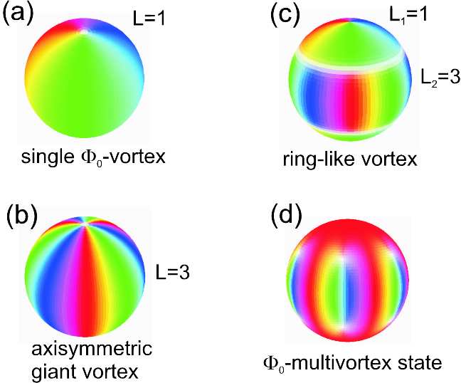
Figure 1: A few examples of vortex structures on a spherical shell are illustrated in this figure, to clarify the nomenclature used in the text. The amplitude and phase of the order parameter are shown as the saturation and hue of the color scale, respectively, in such a way that the vortex core region is white. Panel (a) shows a single $\Phi_{0}$-vortex. In panel (b) a giant vortex (carrying multiple quanta of flux) is depicted. Panel (c) illustates a ring-like vortex separating regions with different angular momentum. Finally, panel (d) shows the $\Phi_{0}$-multivortex state, where an array of singly-quantized vortices is present.

II.1 Giant vortex states

First, let us consider superconducting states, which keep the axial symmetry of the system, so that the order parameter $\psi$ can be written in the form $\psi=f(\theta)\mathrm{exp}(iL\phi)$. where $L$ has the sense of the winding number (vorticity). Then for a stationary distribution $f(\theta)$ the Ginzburg-Landau equation (1) reduces to the one-dimensional equation

$$\frac{\partial^{2}f}{\partial\theta^{2}}+\cot\theta\frac{\partial f}{\partial\theta}-\left(\frac{L}{\sin\theta}-{\eta\sin\theta}\right)^{2}f+2\rho^{2}f(1-f^{2})=0$$ (4)

with boundary conditions, determined by the requirement that the $\theta$-component of the current density must be zero at the $z$-axis: $\left.{\partial f}/{\partial\theta}\right|_{\theta=0,\pi}=0$. Solid lines in Fig. 2 illustrate typical behavior of the free-energy difference $\Delta G$ as a function of $\eta$ for cylindrically symmetric states with different vorticity $L$. In the case of a thin spherical shell with $\rho=8$, as illustrated in panel (a) of Fig. 2, the value of $L$ in the lowest cylindrically symmetric state increases with $\eta$ from 0 at $\eta=0$ to 9 at $\eta=12.5$. The modulus $f$ and phase $L\phi$ are illustated in panel (b) of Fig. 1, using hue and saturation of the color scale respectively. An increase of the applied magnetic field is seen to result also in a significant increase of the Gibbs free energy of the lowest state.

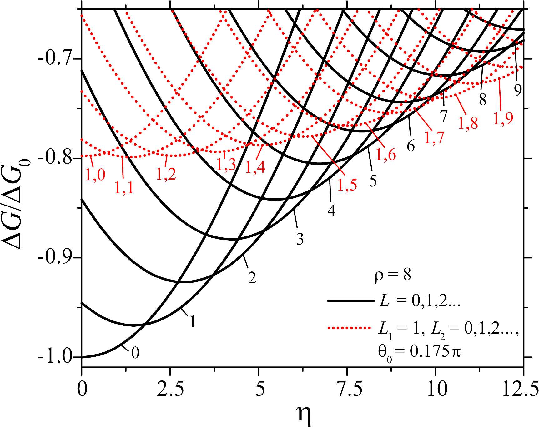
Figure 2: The free energy difference is shown as a function of $\eta$, the number of flux quanta that pass through the equatorial plane of the sphere with radius $\rho=8$, for axially symmetric states. The black solid curves are for states with uniform vorticity (and a giant vortex). The red dotted lines are for states with ring-like vortices.

II.2 Ring-like vortices

In Ref. Zhao , when analyzing supercondicting states in hollow cylinders, it was suggested that – under certain conditions – cylindrically symmetrical states with changing winding number can be more energetically favorable than the states with uniform $L$. Our calculations show that a similar situation occurs also in thin spherical shells with the dimensionless size larger than $\rho\approx 6$ (i.e., for $\mathcal{R}\gtrsim 8.5\xi$), but as we will show in the next section, such states decay into a lattice of singly-quantized vortices breaking the cylindrical symmetry.

We have compared the Gibbs free energies for axially symmetric states with uniform winding number $L$ and those for states where $L_{1}$, the winding number at $0\leq\theta<\theta_{0}$ and $\pi-\theta_{0}<\theta\leq\pi$, differs from $L_{2}$, the winding number at $\theta_{0}<\theta<\pi-\theta_{0}$. The order parameter of the latter states on the sphere are illustrated in panel (c) of Fig. 1 – we will refer to such states as “ring-like vortex” states. The continuity of the order parameter as a function of $\theta$ requires vanishing $f(R,\theta)$ at the boundaries between regions with different winding numbers, i.e., at $\theta=\theta_{0}$ and $\theta=\pi-\theta_{0},$ as can be seen in panel (c) of Fig. 1. At sufficiently strong magnetic fields the Gibbs free energy for states with ring-like vortices can become lower than that for states characterized by a unique winding number $L$ over the whole $\theta$ range. This is illustrated by Fig. 2, where the dotted lines show the calculated free-energy difference $\Delta G(\eta)$ for states with $L_{1}=1$ and different $L_{2}$ on a shell with $\rho=8$ in the case of $\theta_{0}=0.175\pi$. It is worth mentioning that the values $\theta_{0}^{\mathrm{(min)}}$, which minimize $\Delta G$ for the lowest ring-like vortex state at a given $\eta$, are rather insensitive to the dimensionless nanoshell size $\rho$ (at least, for $\rho\leq 10$). At the same time, the parameter $\theta_{0}^{\mathrm{(min)}}$ is an increasing function of $\eta$. Thus, our calculations show that this parameter changes from $\theta_{0}^{\mathrm{(min)}}\approx 0.12\pi$ to $\theta_{0}^{\mathrm{(min)}}\approx 0.2\pi$ when increasing $\eta$ from 7 to 15. However, moderate variations of $\theta_{0}$ around $\theta_{0}^{\mathrm{(min)}}$ only slightly affect $\Delta G$ for the lowest state with ring-like vortices. That is why in Fig. 2 we restricted ourselves to the case of a fixed value $\theta_{0}=0.175\pi$, which coincides with $\theta_{0}^{\mathrm{(min)}}$ at $\eta=10$.

In Fig. 2, the curve labeled with ‘1,1’ corresponds to the state with a ring-like vortex and uniform vorticity, which is qualitativley similar to the states analyzed in Ref. StenuitPC332, . The free energy of this state is always significantly higher than $\Delta G$ for the lowest giant vortex states with point-like core. As can be further seen from Fig. 2, at $\eta\geq 10$ the ring-like vortex states ($L_{1}\neq L_{2}$) appear the most energetically favorable among the axially symmetric states. Thus, at $\eta\geq 12.5$, the difference in $\Delta G/\Delta G_{0}$ between the state with $L=9$ and the state with $L_{1}=1$, $L_{2}=9$ is larger than 0.025. At even larger values of $\eta$, states with three different regions of vorticity $L_{1},L_{2},L_{3}$ (characterized by two ring-like vortices) can become stable. However, our calculations show that in shells with $\eta\gtrsim 6$, where such ring-like vortices allow for decreasing the free energy of giant vortex states as compared to the case of a giant vortex, even lower values of $\Delta G$ can be achieved by breaking up the ring like vortex (or vortices) into an array of singly-quantized vortices. A natural question arises of how stable are the aforedescribed giant vortex states with respect to decay into multiple singly quantized vortices. In order to answer this question, one has to return to the TDGL equation (1).

II.3 Numerical treatment

The finite-difference scheme, applied here to solve Eq. (1), is similar to that of Ref. kato91, , with necessary adaptations to the case of a spherical 2D-system. Two-dimensional grids, used in our calculations, typically have $\gtrsim 100$ equally spaced nodes in the $\theta$-interval from 0 to $\pi$ and $\gtrsim 150$ equally spaced nodes in the $\phi$-interval from 0 to $2\pi$. Cyclic boundary conditions for $\psi$ are applied at $\phi=0$ and $\phi=2\pi$. The boundary conditions at $\theta=0$ and $\theta=\pi$ are determined by the requirement $\left.\psi\right|_{\theta=0,\pi}=\mathrm{const}(\phi)$. The step of the time variable $\tau$ is automatically adapted in the course of calculation. This adaptation is aimed to minimize the number of steps in $\tau$, necessary for approaching a steady solution of Eq. (1), and – at the same time – to keep the solving procedure convergent. On average, the step in $\tau$ is $\sim 10^{-5}$ to $\sim 10^{-4}$ depending on the used grid as well as on $\rho$ and $\eta$. When starting at $\tau=0$ from a random distribution of $\psi$ (with $|\psi|\ll 1$), a (meta)stable solution of Eq. (1) is achieved typically at $\tau\lesssim 100$. When analyzing (meta)stability of states in a spherical shell, one has to keep in mind that a transition between states with different vorticity, in general, requires symmetry breaking. This means that simulations, which assume a perfectly symmetric spherical nanoshell, would tend to overestimate stability of a state with respect to a possible transition to another state with lower free energy. In order to model the effect of imperfections, inevitably present in realistic nanoshells, we consider spherical shells with small angular variations $\delta\rho(\theta,\phi)$ of the parameter $\rho$. Importantly, for relative magnitudes $|\delta\rho|/\rho$ ranging roughly from $\sim 10^{-8}$ to $\sim 10^{-3}$, the results of simulations practically do not depend on a specific choice of the magnitude and distribution of these non-homogeneities. An appreciable effect of those imperfections on stable distributions of the order parameter appears only for $|\delta\rho|/\rho>0.1$.

III Results and discussion for thin shells

III.1 Decay of giant and ring-like vortices

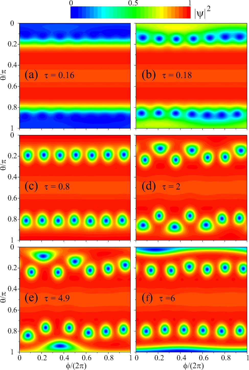
Figure 3: Evolution of the angular distribution of the squared modulus of the order parameter in a thin spherical superconducting shell with $\rho=8$ at $\eta=10$ in the case when the initial state (at $\tau=0$) is a giant vortex with $L=7$. Different panels correspond to different time $\tau$.

In order to examine the stability of giant vortex states with respect to decay into multivortex states, we apply the computation scheme described in the previous section, starting at $\tau=0$ from a distribution of $\psi$ that corresponds to a giant or ring-like vortex state. Typical examples of the evolution of the order parameter distributions are shown in Figs. 3 and 4 for the cases when the initial state is a giant vortex and a ring-like vortex, respectively. In the case of $\rho=8$ and $\eta=10$, the thermodynamically stable state corresponds to 7 pairs of vortices with a single quantum $\Phi_{0}$ of flux each, and it has a relative free energy $\Delta G/\Delta G_{0}\approx-0.812$, approximately 0.07 lower than the value of $\Delta G/\Delta G_{0}$ for the lowest giant vortex state (see Fig. 2). Such lattices of vortices with each a singly flux quantum $\Phi_{0}$ will be denoted as “$\Phi_{0}$-multivortex states”.

As illustrated by Figs. 3(a) to 3(c), within a $\tau$-interval $\sim 1$ the initial giant vortex state with $L=7$ transforms into a chain of 7 singly quantized vortices, which surround each pole of the sphere. In the course of the further rearrangement of the vortex pattern, one of the vortices moves to the pole, while the remaining 6 vortices tend to form a symmetric chain around the pole (see Figs. 3(d) to 3(f)). A free-energy gain due to this rearrangement is by one order of magnitude smaller than that due to the decay of the initial giant vortex into single vortices. Correspondingly, the $\tau$-interval, necessary for this rearrangement, appears to be relatively long: only at $\tau\approx 10$ the solution reaches the equilibrium symmetric configuration of vortices (not shown in Fig. 3), similar to that found in Ref. Du04, , where $\Phi_{0}$-multivortex states on a thin hollow sphere were studied in detail. As seen from Fig. 4, the transition from a ring-like vortex state ($L_{1}=1$ for $0\leq\theta/\pi<0.175$ and $0.825<\theta/\pi\leq 1$; $L_{2}=7$ for $0.175\leq\theta/\pi\leq 0.825$) to a $\Phi_{0}$-multivortex state is even faster. The ring-like vortex core, which is present in the initial state [see Fig. 4(a)], decays into a chain of 6 single vortices very quickly: clear signatures of this decay can be found already at $\tau<0.01$ [see Fig. 4(b)]. The equilibrium state with a vortex at the pole and 6 vortices, symmetrically surrounding the pole, is formed already at $\tau=0.2$.

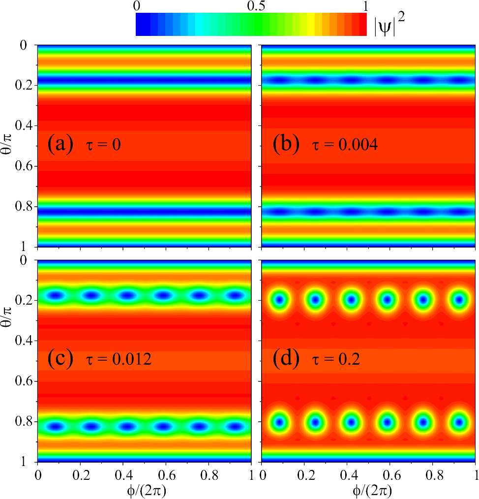
Figure 4: Evolution of the angular distribution of the squared modulus of the order parameter in a thin spherical superconducting shell with $\rho=8$ at $\eta=10$ in the case when the initial state (at $\tau=0$) is a ring-like vortex state with $L_{1}=1$ for $0\leq\theta/\pi<0.175$ and $0.825<\theta/\pi\leq 1$; $L_{2}=7$ for $0.175\leq\theta/\pi\leq 0.825$. Different panels correspond to different time $\tau$.

The results of our calculations clearly indicate that giant and ring-like vortex states are rather unstable in spherical shells with relatively large $\rho$. This does not mean, however, that giant vortex states on a spherical shell are never stable. A decrease of the shell radius and/or an increase of the applied magnetic field enhance the role of the Lorenz forces, which act on the supercurrents and tend to drive vortices towards the poles of the shell. As a result, for sufficiently small $\rho$ and sufficiently large $\eta$, the distance between vortex cores in a $\Phi_{0}$-multivortex state becomes so small, that physically a $\Phi_{0}$-multivortex state appears undistinguishable from the corresponding giant vortex state. A similar continuous transition from a $\Phi_{0}$-multivortex state to a giant vortex states with increasing magnetic field was recently found when solving the linearized Ginzburg-Landau equation for superconducting spherical grains Baelus . Of course, in the case of such a continuous transition, the boundary between thermodynamically stable $\Phi_{0}$-multivortex states and giant vortex states can be drawn only approximately. As a criterion of a transition from a multivortex state to a giant vortex state, here we have chosen the condition that the angular distance of vortex cores from the pole becomes smaller than $(10\rho)^{-1}$.

III.2 Phase diagram for thin shells

Our results, related to thermodynamically stable states on thin spherical shells, are summarized in Fig. 5, where the solid lines indicate boundaries of stability regions for the normal state, the superconducting Meissner states, single $\Phi_{0}$-vortex states, giant vortex and $\Phi_{0}$-multivortex states. The dashed line indicates the boundary between the regions, where giant vortex states (to the left from this line) or $\Phi_{0}$-multivortex states (to the right from this line) are thermodynamically stable. As seen from Fig. 5, formation of vortices can be energetically advantageous only on sufficiently large shells: at $\rho\geq 0.63$ for states with $L=1$, at $\rho\geq 0.85$ for giant vortex states, and at $\rho\geq 1.95$ for $\Phi_{0}$-multivortex states.

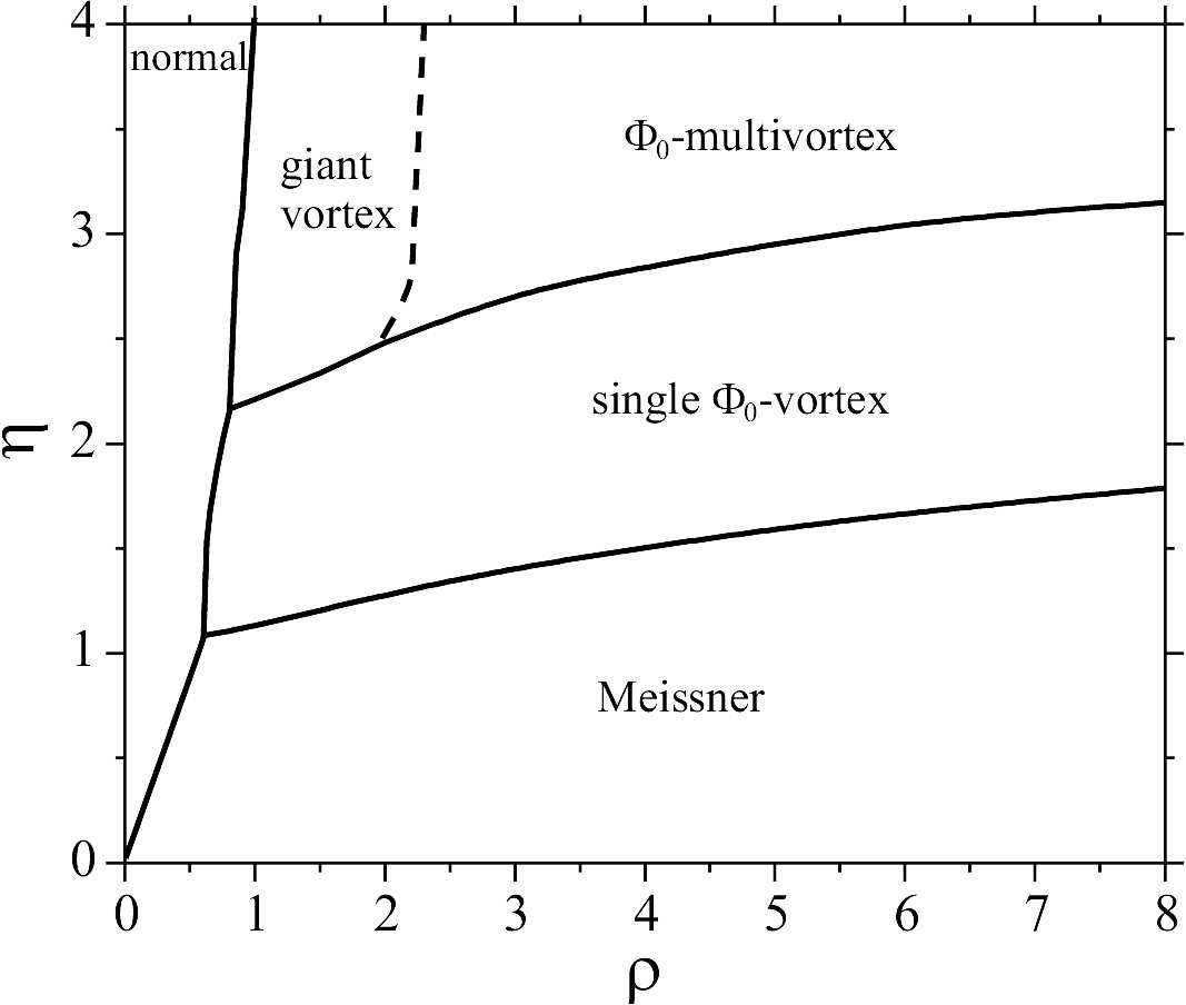
Figure 5: Phase diagram for thin spherical superconducting shells in the $(\rho,\eta)$-plane. The boundaries between the regions with the thermodynamically stable normal state, the Meissner state, the single $\Phi_{0}$-vortex state, giant vortex state, and $\Phi_{0}$-multivortex states are shown by solid lines. The dashed line approximately indicates the boundary between the regions, where giant vortex states or $\Phi_{0}$-multivortex states are the thermodynamically stable state.

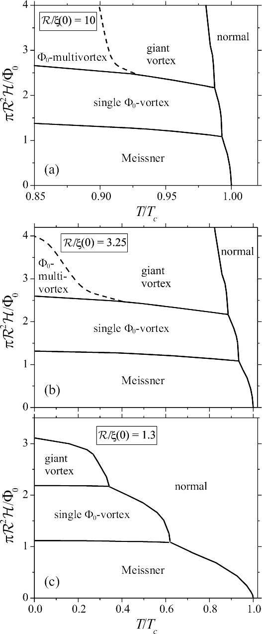
Figure 6: Phase boundaries for thin spherical superconducting layers with different radius $\mathcal{R}$ as a function of the temperature $T$ and the applied magnetic field $\mathcal{H}$. Boundaries between the thermodynamically stable normal state, Meissner state, single $\Phi_{0}$-vortex state, giant vortex state, and $\Phi_{0}$-multivortex states are shown by solid lines. The dashed line approximately indicates the boundary between the regions, where giant vortex states or $\Phi_{0}$-multivortex states are the thermodynamically stable state.

While in Fig. 5 the phase diagram for thin spherical superconducting shells is shown in the $(\rho,\eta)$-plane, it seems interesting to analyze the phase boundaries also in more common form: in terms of the applied magnetic field $\mathcal{H}$ and the temperature $T$. We assume that the temperature dependence of the penetration depth $\lambda$ is described by the empirical relation $\lambda(T)=\lambda(0)/\sqrt{1-(T/T_{c})^{4}}$, while the (less important) temperature dependence of the Ginzburg-Landau parameter $\kappa$ is roughly given by the expression $\kappa(T)=\kappa(0)/[1+(T/T_{c})^{2}]$ (see, e.g., Ref. Tinkham, ). In Fig. 6 we plot the phase boundaries for thermodynamically stable normal states, Meissner states, single $\Phi_{0}$-vortex, giant vortex, and $\Phi_{0}$-multivortex states on spherical superconducting shells with different radius $\mathcal{R}$, measured in units of the zero-temperature Ginzburg-Landau coherence length $\xi(0)$. As illustrated in Fig. 6(a), in the case, where the radius $\mathcal{R}$ is much larger than $\xi(0)$, giant vortex states are thermodynamically stable (at moderate applied magnetic fields) only in the close vicinity of the critical temperature $T_{c}$. With decreasing $\mathcal{R}$, the stability range of giant vortex states gradually extends towards lower temperatures and lower values of the magnetic flux through the shell. Correspondingly, in sufficiently small shells the stability range of $\Phi_{0}$-multivortex states is restricted to a relatively narrow interval of $\mathcal{H}$ and to $T$, significantly lower than $T_{c}$ [see Fig. 6(b)]. On even smaller shells (with $\mathcal{R}$ close to $\xi(0)$) no stable $\Phi_{0}$-multivortex states are possible [see Fig. 6(c)]. For those small shells, the superconducting phase persists only for relatively weak (few $\Phi_{0}$) magnetic fluxes through the shell. At the same time, as implied by a comparison between panels (b) and (c) in Fig. 6, the values of the applied magnetic field $\mathcal{H}$, which correspond to transitions with an increase of vorticity by 1, become significantly higher when decreasing the shell size.

IV Vortex states on thick shells

IV.1 Magnetization effects in thick shells

Now, let us extend our analysis to the case of relatively thick spherical shells, where magnetic fields, induced by supercurrents, which flow in a shell, are of non-negligible. At the same time, we assume that the thickness of a shell is still sufficiently small for neglecting variations of the order parameter $\psi$ and of the vector potential $\mathbf{A}=\mathbf{A}_{0}+\mathbf{A}_{1}$ across the layer. For such a shell, also currents across the layer can be neglected. Expressing the vector potential $\mathbf{A}_{1}$ through the density of current $\mathbf{j}$ as

$$\mathbf{A}_{1}(\mathbf{r})=\frac{1}{2\pi}\int d^{3}r^{\prime}\frac{\mathbf{j}(\mathbf{r}^{\prime})}{|\mathbf{r}-\mathbf{r}^{\prime}|}.$$ (5)

the non-negligible components of the product $R\mathbf{A}_{1}$, which enters Eq. (1), can be written down in the following form:

$$R{A}_{1\theta} = \frac{WR}{2\sqrt{2}\pi}\int\limits_{0}^{\pi}d\theta^{\prime}\sin\theta^{\prime}\int\limits_{0}^{2\pi}d\phi^{\prime}\left\{\left[\sin\theta\mathrm{sin}\theta^{\prime}+\cos\theta\cos\theta^{\prime}\cos\left(\phi-\phi^{\prime}\right)\right]Rj_{\theta^{\prime}}\left(\theta^{\prime},\phi^{\prime}\right)\right.$$ (6)

$$\left.+\cos\theta\sin\left(\phi-\phi^{\prime}\right)Rj_{\phi^{\prime}}\left(\theta^{\prime},\phi^{\prime}\right)\right\}\left[1-\cos\theta\cos\theta^{\prime}-\sin\theta\sin\theta^{\prime}\cos\left(\phi-\phi^{\prime}\right)\right]^{-1/2},$$

$$R{A}_{1\phi} = \frac{WR}{2\sqrt{2}\pi}\int\limits_{0}^{\pi}d\theta^{\prime}\sin\theta^{\prime}\int\limits_{0}^{2\pi}d\phi^{\prime}\left\{\cos\theta^{\prime}\sin\left(\phi^{\prime}-\phi\right)Rj_{\theta^{\prime}}\left(\theta^{\prime},\phi^{\prime}\right)\right.$$ (7)

$$\left.+\cos\left(\phi-\phi^{\prime}\right)Rj_{\phi^{\prime}}\left(\theta^{\prime},\phi^{\prime}\right)\right\}\left[1-\cos\theta\cos\theta^{\prime}-\sin\theta\sin\theta^{\prime}\cos\left(\phi-\phi^{\prime}\right)\right]^{-1/2},$$

where $W$ is the dimensionless thickness of the shell. On the other hand, in the case of constant or slowly varying magnetic fields, using the relation

$$\mathbf{j}=\mathrm{Re}\left[\psi^{*}\left(\frac{\bigtriangledown}{i}-\mathbf{A}\right)\psi\right],$$ (8)

the products $Rj_{\theta}$ and $Rj_{\phi}$, which enter Eqs. (6) and (7), can be expressed through $\psi$, $R{A}_{\theta}$, and $R{A}_{\phi}$ as

$$Rj_{\theta}=\mathrm{Im}\left[\psi^{*}\frac{\partial\psi}{\partial\theta}\right]-R{A}_{1\theta}|\psi|^{2},$$ (9)

$$Rj_{\phi}=\frac{1}{\sin\theta}\mathrm{Im}\left[\psi^{*}\frac{\partial\psi}{\partial\phi}\right]-\left(\eta\sin\theta+R{A}_{1\phi}\right)|\psi|^{2}.$$ (10)

In order to find the order parameter $\psi$ and the corresponding vector potential, we solve self-consistently the set of equations (1), (6), and (7), using relations (9), and (10). From Eqs. (1), (6), (7), (9), and (10), one can see that for relatively thick shells under consideration a set of independent parameters, which govern the solution, can be chosen as $\eta$, $\rho$, and $\omega$, where the introduced additional parameter $\omega\equiv WR=\mathcal{WR}/(2\lambda^{2})$ is linearly proportional to the thickness of the nanoshell and to its radius.

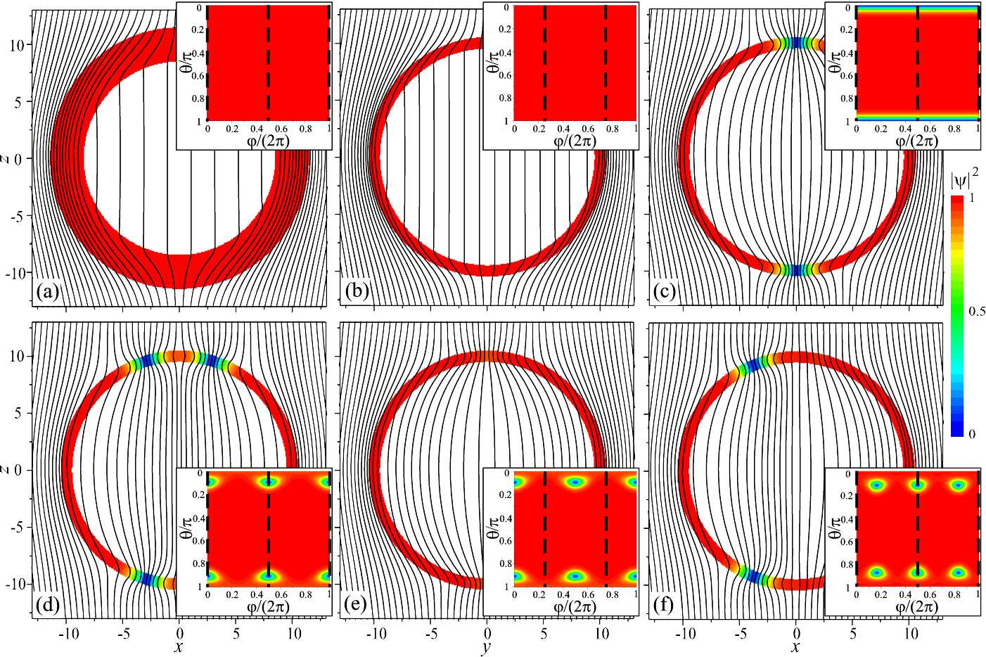
Figure 7: Magnetic-field lines and distribution of the squared modulus of the order parameter for thermodynamically stable states in superconducting spherical shells with $\kappa=0.8$, $R=10$, $W=3$ [panel (a)] and $\kappa=0.8$, $R=10$, $W=1$ [panels (b) to (f)]. The results are shown for the $xz$-cross-section [panels (a), (c), (d), (f)] and the $yz$-cross-section [panels (b), (e)] of the shell for different values of the parameter $\eta$ and vorticity $L$: $\eta=5$, $L=0$ [panels (a) and (b)], $\eta=6.5$, $L=1$ [panel (c)], $\eta=8$, $L=2$ [panels (d) and (e)], $\eta=9.5$, $L=3$ [panel (f)]. Insets: angular distributions of the squared modulus of the order parameter for the same values of $\eta$ and other parameters. Vertical dashed lines on each inset correspond to the cross-section displayed on the main panel.

Figure 7 gives few examples of magnetic-field distributions, which correspond to thermodynamically stable states in spherical shells with $\rho=8$, $\omega=30$ and $\rho=8$, $\omega=10$. The patterns of magnetic-field lines, displayed in Fig. 7, are plotted for the particular case of the Ginzburg-Landau parameter $\kappa=0.8$, the (mean) dimensionless radius of the shell $R=10$, and the dimensionless thickness $W=3$ and $W=1$. In general, none of the three mutually orthogonal components of the magnetic field $\mathbf{B}=\mathbf{\nabla}\times\mathbf{A}$ is zero, so that the field lines are “three-dimensional”. In Fig. 7, however, we restrict ourselves to field-line patterns within symmetry planes, where the field lines are “flat”. As seen from Fig. 7(a), even in the case of a relatively thick shell ($W=3$) the magnetic fields, induced by the supercurrents in the Meissner state, are not sufficient for complete screening of the applied magnetic field inside the shell. Nevertheless, not only in the case of $W=3$ but also for a significantly thinner shell with $W=1$ [Fig. 7(b)], the net field inside the shell is much weaker than $H$. In the case of the state with $L=1$, the magnetic flux, captured by a vortex pair, is seen as an increased density of field lines at the poles of the sphere [Fig. 7(c)]. At the same time, in the depth of the sphere the magnetic field is relatively homogeneous, only slightly increasing towards the $z$-axis. Also for states with higher vorticity, a considerable local increase of the magnetic-flux density takes place only at the vortex cores within the superconducting shell, while in the depth of the sphere the density of magnetic-field lines is considerably more homogeneous [see panels (d) to (f) in Fig. 7].

IV.2 Phase diagram for thick shells

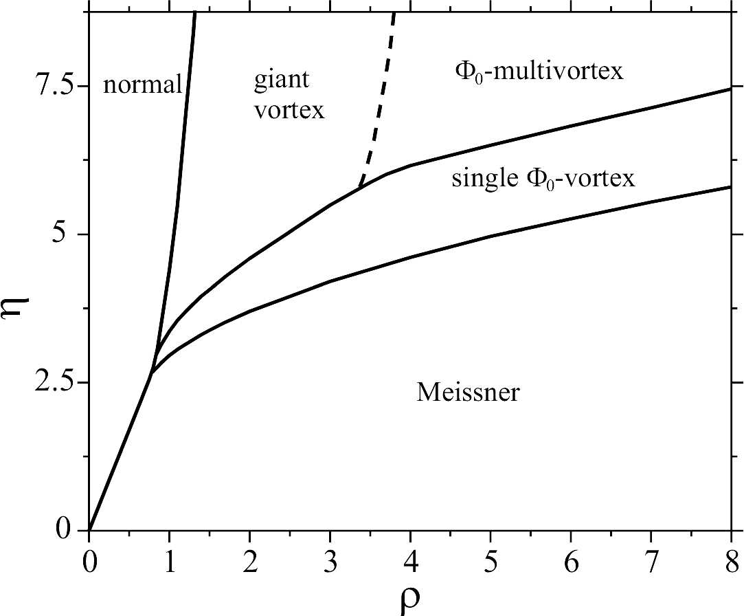
Figure 8: Phase diagram for thick ($\omega=10$) spherical superconducting shells in the $(\rho,\eta)$-plane. The boundaries between the thermodynamically stable normal state, Meissner state, single $\Phi_{0}$-vortex state, giant vortex state, and $\Phi_{0}$-multivortex states are shown by solid lines. The dashed line approximately indicates the boundary between the regions, where giant vortex states or $\Phi_{0}$-multivortex states are the thermodynamically stable state.

As seen from Fig. 7, the magnetic fields, induced by supercurrents, can be considerably large even for shells with quite moderate thickness ($W\sim 1$). These fields strongly affect the stability range for superconducting states with different vorticity in a spherical shell. In Fig. 8, we present the calculated phase diagram for relatively thick spherical shells with $\omega=10$. As follows from a comparison of Fig.  8 to Fig. 5, an increase of the thickness of a spherical shell results in a well-pronounced shift of the boundaries between states with different vorticity towards higher magnetic fields $\eta$. In particular, for $\rho>0.8$, the range of $\eta$, where Meissner states are thermodynamically stable, is more than two times wider in the case of $\omega=10$ as compared to the case of $\omega\rightarrow 0$. One can also see that for a relatively thick spherical shell ($\omega=10$) the boundary between giant vortex and $\Phi_{0}$-multivortex states is shifted towards significantly larger values of $\rho$ as compared to those in the case of $\omega\rightarrow 0$. The increased stability of giant vortex states agree with the results recently obtained by Baelus et al. Baelus for the limit $W\rightarrow R$ of a full sphere, in the framework of linearized Ginzburg-Landau equations.

In Fig. 9 the phase boundaries for thermodynamically stable normal states, Meissner states, single $\Phi_{0}$-vortex, giant vortex, and $\Phi_{0}$-multivortex state states are plotted in the $(T,\mathcal{H})$-plane. The results are shown for shells with different radius $\mathcal{R}$ and thickness $\mathcal{W}$. In order to keep the plots more universal, it is convenient to express the thickness in units of $\xi(0)\kappa^{2}(0)$. For thick nanoshells, there is a much more pronounced increase of the transition fields, which correspond to a change of vorticity, with lowering temperature [cp. Figs. 9(a) and 9(c) to Figs. 6(a) and 9(c)]. When comparing Fig. 9(a) to Fig. 6(a) one can also see that with increasing the nanoshell thickness the temperature range, where giant vortices are thermodynamically stable, extends towards lower temperatures. With decreasing the shell radius, this effect becomes quite pronounced even for relatively small values of $\mathcal{W}/[\xi(0)\kappa^{2}(0)]$ [cp. Fig. 9(b) to Fig. 6(b)]. In sufficiently thick nanoshells, the temperature range, where $\Phi_{0}$-multivortex states are thermodynamically stable, reduces to zero [see Fig. 9(c)], although in thin nanoshells of the same radius this range is relatively wide [see Fig. 6(b)]. Of course, when the temperature approaches $T_{c}$, the phase boundaries become almost insensitive to the value of $\mathcal{W}$. Indeed, at $T\rightarrow T_{c}$ the parameter $\omega$ always goes to zero [due to an increase of the penetration depth $\lambda(T)$], so that any nanoshell appears effectively thin.

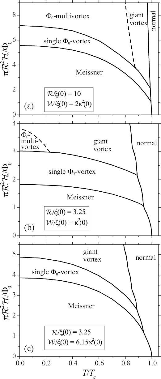
Figure 9: Phase boundaries for spherical superconducting layers with different radius $\mathcal{R}$ and thickness $\mathcal{W}$ as a function of the temperature $T$ and the applied magnetic field $\mathcal{H}$. The boundaries between the thermodynamically stable normal state, Meissner state, single $\Phi_{0}$-vortex state, giant vortex state, and $\Phi_{0}$-multivortex states are shown by solid lines. The dashed line approximately indicates the boundary between the regions, where giant vortex states or $\Phi_{0}$-multivortex states are the thermodynamically stable state.

V Conclusions

Curving a superconducting film into a spherical shell changes its vortex-related properties drastically due to topological constraints. The hairy-sphere theorem Brouwer is a straightforward example of such a constraint: it states that, in contrast to the situation on a flat film, there exists no nonvanishing continuous tangent vector field on the sphere. So, every nonvanishing supercurrent velocity field requires discontinuities, such as vortices. The interplay between the Lorentz force due to an applied field and the vortex superflow will force these vortices away from the equator (leaving an equatorial “Meissner band”) and towards the poles. This results in a ‘polar trapping potential’, which is nearly quadratic near the poles. When vortices conglomerate at the poles, they may coalesce to form giant or ring-like vortices, and these dynamics and phases are the topic of the present paper.

Three contributions to the energy should be kept in mind to interpret the phase diagrams obtained in our calculations. First, to create a vortex, the kinetic energy of the associated supercurrent (on the 2D spherical surface) should be taken into account. This contribution increases when two vortices with parallel vorticity are placed near each other, so it acts as a repulsion between the vortices. Thus, it tends to favor splitting of the giant vortices. Second, to create a vortex, the order parameter needs to be suppressed over a region typically of the size of the coherence length. The energy cost associated with this turns out to favor a multiply quantized (giant) vortex over the corresponding $\Phi_{0}$-multivortex state. The energy cost is relatively larger for a smaller sphere, since proportionally a larger fraction of the total order parameter needs to be suppressed. The balance between these two energy contributions can be used to qualitatively understand the phase diagrams that we calculate for thin shells. Indeed, for magnetic fields corresponding to multiple quanta of vorticity, the smaller spheres will favor giant vortices, whereas the larger spheres favor the $\Phi_{0}$-multivortex state. Note that this contribution to the energy strongly disfavors ring-like vortex states.

The third contribution to the energy is related to the gradients in the magnetic field. When the shell is much thinner than the penetration depth, the currents on the shell will not substantially perturb the applied field, and this contribution plays no role. However, for thicker shells, this contribution does become important – as can be seen from Fig. 7, the magnetic field is substantially perturbed. When a $\Phi_{0}$-multivortex lattice is present, the magnetic field flux is concentrated near each vortex core, and shielded in between, leading to a larger magnetic contribution to the energy than for a giant vortex. Thus, for a thick shell, this contribution will favor the giant vortex state. This agrees with our phase diagram showing that the region, where the giant vortex is stable, is growing for thicker shells.

The temperature dependence of the phase diagrams was studied straightforwardly by taking temperature into account through the Ginzburg-Landau parameters. When multiple quanta of vorticity are present, we find that the giant vortex phase forms the preferred high-temperature phase. This offers the prospect of probing a temperature-driven transition between a giant vortex and a $\Phi_{0}$-multivortex state, alongside with a magnetic-field driven transition. Moreover, the vortex dynamics are shown to be not sensitive to moderate imperfections in the shell; the energy contributions discussed here can overcome the pinning potential due to for example thickness inhomogeneities – such pinning potentials have in past experimental work hampered the detection of the giant vortex state. This robustness, together with the tunability of the phase diagram through a limited set of controllable parameters, makes superconducting nanoshells uniquely suited for the study of novel vortex states.

- (1) M. W. Zwierlein, J. R. Abo-Shaeer, A. Schirotzek, C. H. Schunck and W. Ketterle, Nature 435, 1047-1051 (23 June 2005).
- (2) V.V. Moshchalkov, L. Gielen, M. Dhallé, C. Van Haesendonck, Y. Bruynseraede, Nature 361, 617 (1993).
- (3) V. V. Moshchalkov, X. G. Qiu, and V. Bruyndoncx, Phys. Rev. B 55, 11793 (1997).
- (4) V.R. Misko, V.M. Fomin, J.T. Devreese, V.V. Moshchalkov, Phys. Rev. Lett. 90, 147003 (2003).
- (5) G. Stenuit, J. Govaerts, D. Bertrand and O. van der Aa, Physica C 332, 277 (2000); ibid. Phys. Lett. A 267, 56 (2000).
- (6) V. Bruyndoncx, J. G. Rodrigo, T. Puig, L. Van Look, and V. V. Moshchalkov, Phys. Rev. B 60, 4285 - 4292 (1999); R. Jonckheere et al., Phys. Rev. Lett. 85, 1528 (2000); ibid. Phys. Rev. Lett. 86, 1663 (2001); A. Kanda et al., Phys. Rev. Lett. 93, 257002 (2004).
- (7) V.R. Misko, V.M. Fomin and J.T. Devreese, Phys. Rev. B 64 (2001).
- (8) U.R. Fischer and G. Baym, Phys. Rev. Lett. 90, 140402 (2003); P. Engels, I. Coddington, P. C. Haljan, V. Schweikhard, and E. A. Cornell, Phys. Rev. Lett. 90, 170405 (2003).
- (9) R.D. Averitt, D. Sarkar, and N.J. Halas, Phys. Rev. Lett. 78, 4217 (1997); S.J. Oldenburg, R.D. Averitt, S.L. Westcott, and N.J. Halas, Chem. Phys. Lett. 288, 243 (1998).
- (10) C. R. Hu, R. S. Thomson, Phys. Rev. B 6, 110 (1972).
- (11) R. Kato, Y. Enomoto, S. Maekawa, Phys. Rev. B 44, 6916 (1991).
- (12) Hu Zhao, V. M. Fomin, J. T. Devreese, V. V. Moshchalkov, Solid State Commun. 125, 59 (2003).
- (13) Q. Du, L. Ju, J. Comp. Phys. 201, 511 (2004); ibid. Math. Comp. 74, 1257 (2004).
- (14) B. J. Baelus, D. Sun, F. M. Peeters, Phys. Rev. B 75, 174523 (2007).
- (15) M. Tinkham, Introduction to Superconductivity (2nd ed., McGraw-Hill, New York, 1996).
- (16) L. E. J. Brouwer, Mathematische Annalen 71, 97 (1912).