Exact Green’s functions and Bosonization of a Luttinger liquid coupled to impedances.

Abstract

The exact Green’s functions of a Luttinger Liquid (LL) connected to impedances are computed at zero and finite temperature. It is also shown that if the resistances are equal to the characteristic impedance of the Luttinger liquid then the finite Luttinger liquid connected to resistors is equivalent to an infinite Luttinger liquid. Impedance boundary conditions (IBC) include also as a special limit the case of open boundary conditions, which are explicitly recovered. Finally bosonization for a LL with IBC is proven to hold.

I introduction

Bosonization is one of the standard methods for one dimensional quantum field theories mycitation . Discovered independently in condensed matter and high-energy physics it is the main tool which has allowed to construct the concept of ’Luttinger liquid’ inspired by the physics of the Tomonaga and Luttinger Hamiltonians key-2 . The LL is a universality class of 1D critical systems comprising models as important as the Heisenberg spin chain, the Hubbard model or the Calogero-Sutherland model.

Various boundary conditions (abbreviated as BC throughout the paper) have been considered in the past for a LL. The earliest studies focused on the infinite system and the finite-size LL with periodic boundary conditions (PBC). The properties in both cases can be related through a conformal transformation mycitation . In particular the finite-size properties have been very useful in conjunction with numerics for extraction of the LL parameters. Later more general boundary conditions were also considered: for instance twisted boundary conditions (TBC) or open boundary conditions (OBC). TBC led to the discovery of even-odd effects in a LL and periodicity of permanent currents with the flux key-3 . The OBC which allow description of broken chains were found to have a dramatic effect on critical exponents leading to boundary exponents in addition to bulk ones and bridging the physics of the LL to that of boundary conformal field theory key-4 ; key-5 . More recently dissipative boundary conditions were also introduced for the LL and were used to compute transport properties of the LL: they describe the coupling of a LL wire to electrodes; they comprise the so-called ’radiative boundary conditions’ (which relate time and space derivative of the boson fields key-6 ) and a ’chemical potential matching boundary conditions’ key-7 . Other dissipative boundary conditions include the ’Impedance Boundary Conditions’ (IBC) introduced by the author ac : they consist in a LL connected at its boundaries to two impedances. The IBC can actually be shown to encompass both ’radiative boundary conditions’ and ’chemical potential matching boundary conditions’ which constitute special cases of the IBC with boundary impedances set at half-a-quantum of resistance $h/2e^{2}$. key-9

We will deal in the present paper with the following issues for a LL with IBC: (1) computing its exact Green’s functions and two-point correlators; this will pave the groundwork allowing for (2) extending the usual bosonization technique to such a dissipative system.

Indeed there is no reason to believe that bosonization of such a system is a valid procedure: bosonization is well established in the non-dissipative situations (infinite LL, finite-size LL with PBC, TBC or OBC) but a LL connected to resistors is a dissipative system: plasmons have now a finite-lifetime. Actually to the author’s knowledge bosonization has not been shown to be valid for any LL with dissipative boundary condition. One strategy to show the validity of bosonization is to start from fermions and then (by considering the anomalous current algebra of density operators) to transform the fermionic Hamiltonian into a bosonic one mycitation . Such a course is in our case plagued with difficulties related to dissipation: the density eigenmodes of the cavity do not form a neat orthogonal basis of states and do not quantize as free bosons. Such problems are actually symptoms of non-hermitian Hamiltonian physics and the existence of non-trivial self-energies: this is a recurrent issue for open systems which is well-known and has led to recourse to biorthogonal bases of states in such diverse contexts as mesoscopic transport key-11 , laser physics (leaking cavities in QED where quantization of the gauge field in terms of photons breaks down) key-12 , acoustics key-13 , black hole physics key-14 , etc. Biorthogonal bases of states lead however for the bosonization program to unnecessary complications.

Nevertheless it will be shown that bosonization does hold for the model at hand (LL with IBC). Instead of following the afore mentioned strategy for bosonization we will find more convenient to start from a bosonic theory and then fermionize it. As an interesting side result of our proof we will compute the exact Green’s functions and correlators of the boson Hamiltonian. Another interesting side result with potential applications is the finding that with suitably chosen resistances the finite LL with impedance boundary conditions (IBC) is equivalent to an infinite LL (namely by identity of their Green’s functions): in a mesoscopic setting the LL in principle can not be abstracted from its surroundings so that the intrinsic properties of an infinite LL are not directly accessible. We show a conceptually simple way out which exploits the fact that a LL can be viewed as a quantum transmission line.

OBC will also be shown to be a special case of IBC corresponding to infinite resistances.

The paper structure will be as follows:

- (1) in section II we introduce a model of a (fermionic) LL connected to resistors through boundary conditions (impedance boundary conditions IBC); these boundary conditions are then recast equivalently in terms of boundary conditions for chiral bosons.

- (2) In the next two sections III and IV we next focus on the bosonic model and compute exactly its Green’s functions and correlators (at zero and finite temperature). As side results we obtain the exact finite-frequency conductivity of the LL with IBC and we prove the equivalence of an infinite LL to a finite-size LL with IBC with suitably chosen resistances.

- (3) We prove bosonization for our model in section V.

- (4) We compute the fermion correlation functions in VI.

Finally an Appendix (Appendix B) is devoted to the single issue of recovering explicitly the fermionic Open BC and the Green’s function, with results identical to those published in the litterature.

II Model

II.1 Notations and definitions.

Phase fields: We consider throughout the paper the standard LL Hamiltonian which written in terms of the usual phase fields reads:

$$H=\frac{\hbar u}{2}\int_{-L/2}^{L/2}dx\,\,\frac{1}{K}\>\left(\partial_{x}\phi\right)^{2}+K\>\Pi^{2}$$

where the fields $\phi$ and $\Pi$ are canonical conjugates

$$\left[\phi(x,t);\,\Pi(y,t)\right]=i\,\delta(x-y).$$

In terms of fermionic operators the fermion density operator is related to $\phi$ through:

$$\rho-\rho_{0}=\frac{1}{\sqrt{\pi}}\>\partial_{x}\phi.$$

(Of course such an identification is not fully warranted at this stage but we will show later it does hold even for a LL connected to resistors; for the time being we may view the relations as defining abstractly the operator $\rho$ rather than equating it with the operator $\psi^{+}\psi$. Similar remarks apply for all the operators defined for fermions such as current, etc.)

The phase field $\Theta$ is defined per:

$$\Pi=-\partial_{x}\Theta$$

and

$$\left[\phi(x,t);\,\Theta(y,t)\right]=i\,\theta(x-y)$$

where $\theta$ is the Heaviside step function.

Chiral fields: The equations of motion of the phase fields:

$$\partial_{t}\phi = -uK\>\partial_{x}\Theta$$

$$\partial_{t}\Theta = -\frac{u}{K}\>\partial_{x}\phi$$

imply:

$$\partial_{x}\left(\phi\pm K\Theta\right)=\mp\frac{1}{u}\,\partial_{t}\left(\phi\pm K\Theta\right).$$

The fields $\phi\pm K\Theta$ are therefore chiral and we define chiral phase fields and chiral densities:

$$\phi_{\pm} = \frac{\phi\pm K\Theta}{2},$$

$$\rho_{\pm} = \frac{1}{\sqrt{\pi}}\,\partial_{x}\phi_{\pm}.$$

They obey: $\phi_{\pm}(x,t)=\phi_{\pm}(x\mp ut)$. Evidently $\rho-\rho_{0}=\rho_{+}+\rho_{-}$.

Current: The particle current density is:

$$i = -\frac{1}{\sqrt{\pi}}\>\partial_{t}\phi$$

$$= \frac{uK}{\sqrt{\pi}}\>\partial_{x}\Theta$$

$$= u\>(\rho_{+}-\rho_{-})$$

where the first line follows from current conservation and the others from the equations of motion of the phase fields.

Chiral chemical potentials:

We define the following operators $\mu_{\pm}$ (they will prove convenient to define our model):

$$\mu_{\pm}(x,t)=\frac{\delta H}{\delta\rho_{\pm}(x,t)}$$

where functional differentiation with respect to the particle density $\rho_{\pm}(x,t)$ has been performed. Physically they correspond to chemical potential operators: their average value yields the energy needed to add one particle at position $x$ to the chiral density: $\rho_{\pm}\longrightarrow\rho_{\pm}+\delta(x)$. These chiral chemical potentials correspond to the plasma chiral eigenmodes of the Luttinger liquid and not to the left or right moving (bare) electrons. An average chemical potential can be defined also as:

$$\mu=\frac{\mu_{+}+\mu_{-}}{2}.$$

From their definition it follows that:

$$\mu_{\pm}=\frac{hu}{K}\,\rho_{\pm},$$ (1)

where we used the relation:

$$H=\frac{\pi\hbar u}{K}\int_{-L/2}^{L/2}dx\>\rho_{+}^{2}+\rho_{-}^{2}.$$

Therefore the electrical current $i_{e}=e\>i$ :

$$i_{e}(x,t) = K\frac{e}{h}\left(\mu_{+}-\mu_{-}\right)$$ (2)

$$= \frac{1}{2Z_{0}}\,\left(\frac{\mu_{+}}{e}-\frac{\mu_{-}}{e}\right)$$

where we have introduced the characteristic impedance of the LL:

$$Z_{0}=\frac{h}{2Ke^{2}}.$$

As explained in ac the LL Hamiltonian is identical with that of a quantum transmission line with a characteristic impedance $Z_{0}$ given as above.

II.2 Model.

Our model consists in a LL connected in series with two impedances. We will use a description of the LL connected to reservoirs ac which is the exact implementation of the load impedances boundary conditions customary for transmission lines or sound waves in tubes.

We thus assume the following boundary conditions:

$$Z_{S}\>i_{e}(-L/2,t) = V_{S}(t)-\frac{\mu(-L/2,t)}{e},$$ (3)

$$Z_{D}\>i_{e}(L/2,t) = \frac{\mu(L/2,t)}{e}-V_{D}(t).$$

$Z_{S}$ and $Z_{D}$ are interface impedances (at respectively the source and the drain) which for simplicity will be assumed to be positive real numbers throughout the paper (in other words they represent resistors; but more general situations could be discussed with complex impedances, which is why we stick in this paper to viewing them as impedances). $i_{e}(x,t)$ is the current operator, and source and drain are set at a voltage $V_{S}$ or $V_{D}$ (see Fig.1). The Heisenberg picture is assumed so that we work with time-dependent operators.

As one can see the boundary conditions are tantamount to assuming Ohm’s law at the boundaries of the system $U=RI$: the current is proportional to a voltage drop between the reservoir and the LL wire and the proportionality constant is just a resistance. In the following the source and drain voltages will be set to zero since we want to compute the equilibrium Green’s function (in the absence of external voltage).

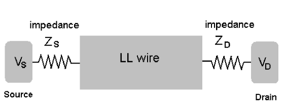
Figure 1: Impedance boundary conditions: the LL wire is connected to two electrodes at voltages $V_{S}$ and $V_{D}$ through two impedances.

It is instructive to recast the (equilibrium) boundary conditions in terms of the chiral densities. This yields:

$$Z_{S}\>u\,e\>\left[\rho_{+}(-L/2)-\rho_{-}(-L/2)\right] = -\frac{hu}{2Ke}\>\left[\rho_{+}(-L/2)+\rho_{-}(-L/2)\right],$$

$$Z_{D}\>u\,e\>\left[\rho_{+}(L/2)-\rho_{-}(L/2)\right] = \frac{hu}{2Ke}\>\left[\rho_{+}(L/2)+\rho_{-}(L/2)\right].$$

So that:

$$\rho_{+}(-L/2) = \frac{Z_{S}-Z_{0}}{Z_{S}+Z_{0}}\>\rho_{-}(-L/2),$$ (4)

$$\rho_{-}(L/2) = \frac{Z_{D}-Z_{0}}{Z_{D}+Z_{0}}\>\rho_{+}(L/2).$$

This introduces reflection coefficients for the density:

$$r_{S}=\frac{Z_{S}-Z_{0}}{Z_{S}+Z_{0}},\quad r_{D}=\frac{Z_{D}-Z_{0}}{Z_{D}+Z_{0}}\text{.}$$ (5)

These expressions deserve some comment: they are just what one would expect for a classical transmission line connected to load and drain impedances. The (classical) equations of motion are indeed also valid at the quantum level since the LL Hamiltonian is quadratic so we might have anticipated any linear relation to carry on. The basic physics of the boundary conditions considered in this paper are therefore those of standing waves in a transmission line produced by reflections at the boundaries due to impedance mismatch.

The reflection coefficients for the phase fields can also be derived; from eq.(4) it follows:

$$\partial_{x}\phi_{+}(-L/2,t) = r_{S}\>\partial_{x}\phi_{-}(-L/2,t),$$ (6)

$$\partial_{x}\phi_{-}(L/2,t) = r_{D}\>\partial_{x}\phi_{+}(L/2,t).$$

The IBC can then be rewritten as conditions on the non-chiral phase field:

$$-Z_{S}\>\frac{1}{u}\partial_{t}\phi(-L/2,t) = Z_{0}\partial_{x}\phi(-L/2,t),$$ (7)

$$Z_{D}\>\frac{1}{u}\partial_{t}\phi(-L/2,t) = Z_{0}\partial_{x}\phi(-L/2,t).$$

As an aside we note that open boundary conditions (OBC) are recovered by setting $r_{S}=r_{D}=1$ (see Appendix B).

III Green’s function of the phase field.

III.1 Green’s function of the phase field $\phi$.

Having derived boundary conditions for the boson fields we now forget the underlying fermions and focus on the following model:

$$H=\frac{\hbar u}{2}\int_{-L/2}^{L/2}dx\,\,\frac{1}{K}\>\left(\partial_{x}\phi\right)^{2}+K\>\Pi^{2}$$

where as before the fields $\phi$ and $\Pi$ are canonical conjugates and:

$$\phi_{\pm}=\frac{\phi\pm K\Theta}{2}.$$

The problem we will tackle is the following: solving for the retarded Green’s function of the bosonic Hamiltonian subjected to the boundary conditions for the fields:

$$\partial_{x}\phi_{+}(-L/2,t) = r_{S}\>\partial_{x}\phi_{-}(-L/2,t),$$

$$\partial_{x}\phi_{-}(L/2,t) = r_{D}\>\partial_{x}\phi_{+}(L/2,t).$$

These boundary conditions introduce dissipation in the problem.

The Green’s function can be conveniently divided into four chiral components: $G_{R}=G_{R}^{++}+G_{R}^{--}+G_{R}^{+-}+G_{R}^{-+}$ where $G_{R}^{\pm\pm}(x,t;y,t^{\prime})=-i\,\theta(t-t^{\prime})\left\langle\left[\phi_{\pm}(x,t),\phi_{\pm}(y,t^{\prime})\right]\right\rangle$ for the retarded Green’s function and appropriate definitions for the advanced Green’s function. Since we will also need the chiral Green’s functions for the bosonization proof instead of directly computing the full Green’s function we will first compute the chiral Green’s functions.

Using the equal-time commutation relations for the chiral fields,

$$\left[\phi_{\pm}(x,t),\phi_{\pm}(y,t)\right] = \pm\frac{iK}{4}\>sgn(x-y),$$

$$\left[\phi_{+}(x,t),\phi_{-}(y,t)\right] =- \frac{iK}{4},$$

one gets the equations of motion for the chiral Green’s functions as:

$$\left[\frac{\partial}{\partial x}\pm\frac{1}{u}\frac{\partial}{\partial t}\right]G^{\pm\pm}(x,t;y,0)=\frac{K}{4u}\,sgn(x-y)\,\delta(t),$$

and:

$$\left[\frac{\partial}{\partial x}\pm\frac{1}{u}\frac{\partial}{\partial t}\right]G^{\pm\mp}(x,t;y,0)=-\frac{K}{4u}\,\delta(t).$$

The impedance boundary conditions imply:

$$\partial_{x}G_{R}^{++} =r_{S}\partial_{x}G_{R}^{-+} ,\;x=-L/2,$$

$$\partial_{x}G_{R}^{+-} =r_{S}\partial_{x}G_{R}^{--} ,\;x=-L/2,$$

$$\partial_{x}G_{R}^{--} =r_{D}\partial_{x}G_{R}^{+-} ,\;x=L/2,$$

$$\partial_{x}G_{R}^{-+} =r_{D}\partial_{x}G_{R}^{++} ,\;x=L/2.$$

After Fourier transforming according to:

$$f(t)=\int_{-\infty}^{\infty}\frac{d\omega}{2\pi}\,f(\omega)\,e^{-i\omega t},$$

and defining $k=\omega/u$ the equations of motion imply the following forms:

$$G^{++} = \theta(x-y)\left(\frac{a^{>}}{ik}\,e^{ikx}-\frac{K}{4i\omega}\right)+\theta(y-x)\left(\frac{a^{<}}{ik}\,e^{ikx}+\frac{K}{4i\omega}\right),$$

$$G^{--} = \theta(x-y)\left(-\frac{b^{>}}{ik}\,e^{-ikx}+\frac{K}{4i\omega}\right)+\theta(y-x)\left(-\frac{b^{<}}{ik}\,e^{-ikx}-\frac{K}{4i\omega}\right).$$

Likewise:

$$G^{+-} = c\,e^{ikx}+\frac{K}{4i\omega},$$

$$G^{-+} = d\,e^{-ikx}-\frac{K}{4i\omega}.$$

The boundary conditions imply the following relations:

$$a^{<} = -ik\,r_{S}\,e^{i\varphi}\,d$$

$$a^{>} = -ik\,r_{D}^{-1}\,e^{-i\varphi}\,d$$

$$b^{<} = ik\,r_{S}^{-1}\,e^{-i\varphi}\,c$$

$$b^{>} = ik\,r_{D}\,e^{i\varphi}\,c.$$

where we have defined a phase $\varphi$ corresponding to the phase accumulated along the wire by the plasma wave:

$$\varphi=kL.$$

Using now the discontinuity of the derivatives of $G^{++}$ and $G^{--}$yields:

$$a^{>}-a^{<} = \frac{K}{2u}\,e^{-iky},$$

$$b^{>}-b^{<} = \frac{K}{2u}\,e^{iky}.$$

Finally:

$$G_{R}^{++}(x,y,\omega) = \frac{K}{2i\omega\left(1-r_{S}r_{D}e^{i2\varphi}\right)}\,e^{i\frac{\omega}{u}(x-y)}\,\left[\theta(x-y)+\theta(y-x)\,r_{S}r_{D}\,e^{i2\varphi}\right]$$

$$-\frac{K}{4i\omega}\,sgn(x-y),$$

$$G_{R}^{--}(x,y,\omega) = \frac{K}{2i\omega\left(1-r_{S}r_{D}e^{i2\varphi}\right)}\,e^{-i\frac{\omega}{u}(x-y)}\,\left[\theta(y-x)+\theta(x-y)\,r_{S}r_{D}\,e^{i2\varphi}\right]$$

$$+\frac{K}{4i\omega}\,sgn(x-y),$$

$$G_{R}^{+-}(x,y,\omega) =- \frac{K}{2i\omega}\,\frac{r_{S}\,e^{i\varphi}}{\left(1-r_{S}r_{D}e^{i2\varphi}\right)}\,e^{i\frac{\omega}{u}(x+y)}+\frac{K}{4i\omega},$$

$$G_{R}^{-+}(x,y,\omega) =- \frac{K}{2i\omega}\,\frac{r_{D}\,e^{i\varphi}}{\left(1-r_{S}r_{D}e^{i2\varphi}\right)}\,e^{-i\frac{\omega}{u}(x+y)}-\frac{K}{4i\omega}.$$

Gathering all terms the full Green’s function is thus:

$$G_{R}(x,y,\omega)=\frac{K}{2i(\omega+i\delta)}\frac{1}{1-r_{S}r_{D}e^{i2\varphi}}$$ (8)

$$\times\left\{\theta(x-y)\left[e^{i\frac{\omega}{u}(x-y)}+r_{S}r_{D}e^{-i\frac{\omega}{u}(x-y-2L)}\right]\right. +\theta(y-x)\left[e^{-i\frac{\omega}{u}(x-y)}+r_{S}r_{D}e^{i\frac{\omega}{u}(x-y+2L)}\right]$$

$$-\left.r_{S}\,e^{i\frac{\omega}{u}(x+y+L)}-r_{D}\,e^{i\frac{\omega}{u}(-x-y+L)}\right\}$$

(where $\varphi=kL$). As a function of time this yields:

$$G_{R}(x,t;y,0)= -\frac{K}{2}\sum_{n=0}^{\infty}(r_{S}r_{D})^{n}\left\{\theta\left(t-\frac{2nL+\left|x-y\right|}{u}\right)+r_{S}r_{D}\theta\left(t-\frac{2(n+1)L-\left|x-y\right|}{u}\right)\right.$$

$$-\left.r_{S}\,\theta\left(t-\frac{(2n+1)L+x+y}{u}\right)-r_{D}\,\theta\left(t-\frac{(2n+1)L-x-y}{u}\right)\right\}$$

For $t<0$, $G_{R}=0$ as it should be.

Technical note: the studious reader interested in deriving directly the advanced Green’s function from the boundary conditions should take note that they must be modified. The reason is simple: a retarded Green’s function which describes outgoing waves (away from the system) are clearly compatible with dissipative BC; but an advanced Green’s function describes incoming waves. So we need BC invariant under time-reversal: to render the time derivative compatible with time-reversal we multiply it by $sgn(t)$

$$-sgn(t)\>Z_{S}\>\partial_{t}\phi(-L/2,\>t) = Z_{0}\partial_{x}\phi(-L/2,t),$$ (9)

$$sgn(t)\>Z_{D}\>\partial_{t}\phi(L/2,\>t) = Z_{0}\partial_{x}\phi(L/2,\>t).$$

In terms of the chiral fields this implies:

$$\partial_{x}\phi_{+}(-L/2,t) = r_{S}^{sgn(t)}\>\partial_{x}\phi_{-}(-L/2,t),$$

$$\partial_{x}\phi_{-}(L/2,t) = r_{D}^{sgn(t)}\>\partial_{x}\phi_{+}(L/2,t).$$

One can check that the BC are now compatible with the usual relation

$$G_{A}(x,t;\,y,0)=G_{R}(y,-t;\,x,0).$$

Note also that the two-point correlators mix advanced and retarded Green’s functions: therefore they will obey these modified boundary conditions as can be readily checked.

III.2 Discussion.

III.2.1 Interpretation.

The interpretation of the Green’s function is quite straightforward: to propagate from one point to the other there are four kinds of basic trajectories (see Figure 2), (1) one can go straight from the starting point to the arrival point, or (2-3) go after bouncing against one of the two boundaries, and (4) lastly go after bouncing two times against different boundaries. These basic trajectories must then be convoluted by round trips along the whole loop (of length $2L$) which yield the overall factor $\left(1-r_{S}r_{D}e^{i2\varphi}\right)^{-1}$ (where $\varphi=\frac{\omega}{u}L$) in the frequency domain expression in eq.(8).

The main difference for the chiral propagators is the appearance of zero modes. The other terms have straightforward interpretations: as before they correspond to straight trajectories from $y$ to $x$ or to propagation with bouncing at either or both of the boundaries. The $\theta(x-y)$ or $\theta(y-x)$ come from the fact that chiral propagation prevents some trajectories depending on the respective positions of $x$ and $y$.

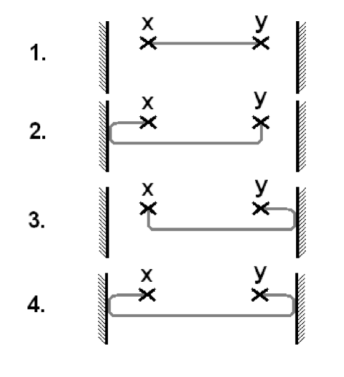
Figure 2: Interpretation of the Green’s function.

We have for now only discussed the retarded Green’s function but of course the advanced Green’s function is simply related to the retarded one through:

$$G_{A}(x,t;\,y,0)=G_{R}(y,-t;\,x,0).$$

So there is no more work to do. The causal Green’s function can also be computed: for instance from the two point correlator (which is discussed later).

We also observe that the retarded and advanced Green’s functions do not depend on temperature since the equation of motion obeyed by the Green’s functions has no temperature dependence. We have therefore found the phase field Green’s functions at all temperatures.

III.2.2 Poles and relation to open boundary LL.

The open boundary conditions (OBC) are a limiting case of the IBC considered in this paper. Hard-walls at the boundaries can be reproduced by considering infinite resistances $Z{}_{S}$ and $Z_{D}$ : this then implies that the reflection coefficients are equal to unity $r_{S}=r_{D}=1$). It can then be checked that our expression for the Green’s function reduces to that found for the LL with open boundary conditions. We refer to Appendix B. Open boundary conditions are actually closely related to the ones discussed in this paper: indeed the excitations in the LL with IBC are those of the LL with OBC albeit with a finite-lifetime. While in the infinite LL or the PBC LL one has travelling waves these excitations are just the standing waves expected from a system enclosed within boundaries.

Indeed the poles are simply:

$$\omega_{n}=\frac{n\pi u}{L}+i\frac{u}{2L}\,\ln(r_{S}r_{D}).$$ (10)

For the OBC there are nodes at the boundaries; the resonances are therefore such that the length of the wire is $L=n\lambda/2$ which leads to $\omega_{n}=\frac{n\pi u}{L}$. Within the simple model of boundary resistances (real positive impedances) the lifetime $\tau=2L/\left(u\>\ln(r_{S}r_{D})\right)$ is independent of the index mode: the level broadening is constant for each standing wave plasma mode. But more complicated situations can be considered: if we assume frequency dependent complex impedances the reflection coefficients then acquire a frequency dependence. This however does not affect the validity of the expressions in the frequency domain just derived for the Green’s function. However the structure of the poles will not be quite as simple as that described above, since the poles are now determined by:

$$1-r_{S}(\omega)r_{D}(\omega)e^{i2L\omega/u}=0.$$

How can we probe these poles? One of the simplest way is through conductivity or conductance measurements. These poles will show up as resonances. Indeed as shown in Appendix A the conductivity is simply:

$$\sigma(x,y,\omega)=\frac{e}{\pi}\,\omega\,G_{R}(x,y,\omega).$$

The conductance (which is a matrix in this context of a gated wire connected to two electrodes) was computed elsewhere ac .

III.2.3 Impedance matching.

Let us recall the basic physics of transmission lines: an ideal transmission line or $LC$-line (e.g. a coaxial cable) has an energy per unit length $\mathcal{E}(x)=\frac{1}{2}\mathcal{L}\,j^{2}(x)+\frac{1}{2\mathcal{C}}\,\rho^{2}(x)$ where $\mathcal{L}$ and $\mathcal{C}$ are respectively an inductance and a capacitance per unit length. For an infinite transmission line the eigenmodes are traveling waves (plasmons) with velocity $u=1/\sqrt{\mathcal{LC}}$. For a finite transmission line connected to two resistors at both boundaries one observes reflections: in general any pulse injected in the transmission line is reflected which leads to energy losses. In order to minimize losses electrical engineers take advantage of the phenomenon of ’impedance matching’: if the resistors have identical resistances equal to $Z_{0}=\sqrt{\mathcal{L}/\mathcal{C}}$ (the characteristic impedance of the transmission line) then the reflection coefficients vanish so that no reflections can occur in the combined system of two resistors+transmission line, which becomes effectively lossless. The finite transmission line has become effectively equivalent to an infinite transmission line. This is the origin of the normalized characteristic impedance of coaxial cables.

What is the relation to the Luttinger liquid ? A LL is actually a quantum transmission line. Indeed its Hamitonian density is just that of a quantum $LC$-line since:

$$H=\intop dx\>\frac{hu}{4K}\,\rho^{2}+\frac{huK}{4}\,j^{2}$$

which rewritten in terms of the charge density and the charge current $\rho_{e}=e\>\rho$ and $j_{e}=euK\>j$ becomes:

$$H=\intop dx\>\frac{\mathcal{L}}{2}\>j_{e}^{2}+\frac{1}{2\mathcal{C}}\>\rho_{e}^{2}$$

with:

$$\mathcal{\mathcal{L}}=\frac{h}{2uKe^{2}},\;\mathcal{C}=\frac{2Ke^{2}}{hu}.$$

So it is only natural to inquire whether the ’impedance matching’ physics is still valid at the quantum level. Quite remarkably it is. We prove the following theorem:

Theorem: the physics of a finite length Luttinger liquid connected to two resistors having resistances equal to the characteristic impedance $Z_{S}=Z_{D}=Z_{0}$ is equivalent to that of an infinite LL (for any observable defined on the length of the LL).

Proof: the proof follows from identity of the Green’s functions. Indeed $Z_{0}=Z_{S}=Z_{D}$ implies: $r_{S}=r_{D}=0$. The expressions of the one-body Green’s functions we have computed then trivially reduce to those of an infinite LL. The N-body Green’s functions are therefore also equal since by Wick’s theorem they reduce to a product of single particle Green’s functions.

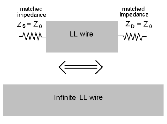
Figure 3: Impedance matching.

Here in the quantum case the cancellation of the reflection coefficients leads to the same physics as in the classical case. Note that the result is still valid if we assume frequency dependent reflection coefficients: if one checks carefully our derivation of the retarded Green’s function in section III one will notice that the expressions do not require frequency-independent coefficients.

Such a result might be useful in any situation where the intrinsic properties of a LL (infinite system) are needed: for transport experiments on quantum wires or carbon nanotubes the coupling to the leads (source and drain) unavoidably modifies the pure physics of the LL. Should one be able to tune the impedance of the leads, one might be able to disenfranchise oneself from the interfering effects of the leads.

In general however the leads will couple to the LL not only with a resistive component but also a capacitive (or even an inductive) component. To achieve perfect impedance matching would mean to be able for all frequency to adjust $Z_{S}(\omega)=Z_{0}=Z_{D}(\omega)$. For all practical purposes depending on the phenomenon one wishes to observe it will be enough to match impedances on a finite window.

Note also that the possibility to match impedances rests crucially on an independent measurement of the characteristic impedance $Z{}_{0}$. This can be achieved through a variety of means: for instance through the finite-frequency conductance as explained by the author in ac or through tunneling experiments.

However it might not be completely necessary to measure the characteristic impedance: one might think of time-resolved experiments where one sends a charged pulse in the wire; if one detects reflected pulses this means that impedances are not matched (actually such tests are routinely used by telecom operators on their transmission lines to find broken lines).

IV Two-point Correlators of the phase fields.

We derive in this sections several correlators at zero and finite-temperature. They will be needed for the proof of bosonization but are also interesting in themselves since they are the building blocks for the vertex operators correlators. All observables of interest can then be calculated: tunneling density of states, current noise, etc.

IV.1 Correlators of the fields $\phi$ and $\Theta$.

It is a simple matter to extract two-point correlation functions; using the definitions of the Green’s functions one has indeed at zero temperature:

$$\left\langle\phi(x,\omega)\phi(y,-\omega)\right\rangle=i\,\theta(\omega)\>\left[G_{R}(x,y,\omega)-G_{A}(x,y,\omega)\right].$$

Tedious but uneventful calculations finally yield the following correlator at zero temperature :

$$F(x,y,t)= \left\langle\phi(x,t)\phi(y,0)\right\rangle$$ (11)

$$= -\frac{K}{4\pi}\;\sum_{n=-\infty}^{+\infty}\left(r_{S}r_{D}\right)^{\left|n\right|} \,\ln\left\{\left[\delta+i(t+\frac{2nL}{u})\right]^{2}+(\frac{x-y}{u})^{2}\right\}$$

$$+ \frac{K}{4\pi}\;\sum_{n=0}^{+\infty}\left(r_{S}r_{D}\right)^{n}\>r_{S} \,\ln\prod_{\varepsilon=\pm 1}\left[\delta+i(t+\varepsilon\frac{x+y+(2n+1)L}{u})\right]$$

$$+ \frac{K}{4\pi}\;\sum_{n=0}^{+\infty}\left(r_{S}r_{D}\right)^{n}\>r_{D} \,\ln\prod_{\varepsilon=\pm 1}\left[\delta+i(t+\varepsilon\frac{x+y-(2n+1)L}{u})\right].$$

Extension to finite-temperature is done by observing that the retarded and advanced Green’s function are temperature independent. Let us consider then the commutator:

$$M(x,t;y,0) = \left\langle\left[\phi(x,t);\,\phi(y,0)\right]\right\rangle.$$

$$= \left\langle\phi(x,t)\,\phi(y,0)-\phi(y,0)\,\phi(x,t)\right\rangle$$

By fluctuation-dissipation (Lehmann’s spectral decomposition):

$$M(x,y,\omega) = (1-e^{-\beta\omega})\left\langle\phi(x,\omega)\,\phi(y,-\omega)\right\rangle_{T}$$

$$= (e^{\beta\omega}-1)\left\langle\phi(y,-\omega)\,\phi(x,\omega)\right\rangle_{T}$$

at temperature $T$. At zero temperature this implies:

$$M(x,y,\omega)=\theta(\omega)\left\langle\phi(x,\omega)\,\phi(y,-\omega)\right\rangle_{0}-\theta(-\omega)\left\langle\phi(y,-\omega)\,\phi(x,\omega)\right\rangle_{0}$$

where the subscript denotes zero temperature. Since $M$ is actually temperature independent, comparison of the two expressions yields:

$$F(x,y,\omega,T)=\left\langle\phi(x,\omega)\,\phi(y,-\omega)\right\rangle_{T}=\frac{1}{1-e^{-\beta\omega}}\left[\theta(\omega)\,F(x,y,\omega,T=0)-\theta(-\omega)\,F(y,x,\omega,T=0)\right]$$

so that the finite-temperature correction is:

$$F(x,y,\omega,T)-F(x,y,\omega,T=0)=\theta(\omega)\,\frac{1}{e^{\beta\omega}-1}\,F(x,y,\omega,T=0)-\theta(-\omega)\,\frac{1}{1-e^{-\beta\omega}}\,F(y,x,\omega,T=0).$$

To regulate the previous correlator one defines: $\widehat{F}_{-+}(x,y,t)=\left\langle\phi(x,t)\,\phi(y,0)\right\rangle-\frac{1}{2}\left\langle\phi^{2}(x,t)+\phi^{2}(y,0)\right\rangle$.

The finite-temperature correlator acquires then a correction from its zero temperature expression $\Delta F=\widehat{F}_{-+}(x,y,t,T)-\widehat{F}_{-+}(x,y,t,T=0)$:

$$\Delta F=-\frac{K}{4\pi}\;\sum_{n=-\infty}^{+\infty}\left(r_{S}r_{D}\right)^{\left|n\right|}\,\ln\left\{\frac{\left|\Gamma\left[1+i\beta^{-1}2nL)\right]\right|^{4}}{\left|\Gamma\left[1+i\beta^{-1}(t+\frac{x-y+2nL}{u})\right]\Gamma\left[1+i\beta^{-1}(t+\frac{y-x+2nL}{u})\right]\right|^{2}}\right\}$$

$$+\frac{K}{4\pi}\;\sum_{n=0}^{+\infty}\left(r_{S}r_{D}\right)^{n}\>r_{S}\>\ln\left\{\frac{\left|\Gamma\left[1+i\beta^{-1}(\frac{2x+(2n+1)L}{u})\right]\right|^{2}\left|\Gamma\left[1+i\beta^{-1}(\frac{2y+(2n+1)L}{u})\right]\right|^{2}}{\left|\Gamma\left[1+i\beta^{-1}(t+\frac{x+y+(2n+1)L}{u})\right]\right|^{2}\left|\Gamma\left[1+i\beta^{-1}(t-\frac{x+y+(2n+1)L}{u})\right]\right|^{2}}\right\}$$

$$+\frac{K}{4\pi}\;\sum_{n=0}^{+\infty}\left(r_{S}r_{D}\right)^{n}\>r_{D}\>\ln\left\{\frac{\left|\Gamma\left[1+i\beta^{-1}(\frac{2x-(2n+1)L}{u})\right]\right|^{2}\left|\Gamma\left[1+i\beta^{-1}(\frac{2y-(2n+1)L}{u})\right]\right|^{2}}{\left|\Gamma\left[1+i\beta^{-1}(t+\frac{x+y-(2n+1)L}{u})\right]\right|^{2}\left|\Gamma\left[1+i\beta^{-1}(t-\frac{x+y-(2n+1)L}{u})\right]\right|^{2}}\right\}$$

where we have made use of the product expansion of the Gamma function $\Gamma$ and $\beta$ is $\frac{1}{T}$. This can also be rexpressed as:

$$\Delta F = -\frac{K}{4\pi}\;\sum_{n=-\infty}^{+\infty}\left(r_{S}r_{D}\right)^{\left|n\right|}\,\ln\left\{\frac{\left[sh_{c}\pi\beta^{-1}(t+\frac{x-y+2nL}{u})\right]\>\left[sh_{c}\pi\beta^{-1}(t+\frac{y-x+2nL}{u})\right]}{\left[sh_{c}\pi\beta^{-1}2nL\right]^{2}}\right\}$$

$$+ \frac{K}{4\pi}\;\sum_{n=0}^{+\infty}\left(r_{S}r_{D}\right)^{n}\>r_{S}\>\ln\left\{\frac{\left[sh_{c}\pi\beta^{-1}(t+\frac{x+y+(2n+1)L}{u})\right]\>\left[sh_{c}\pi\beta^{-1}(t-\frac{x+y+(2n+1)L}{u})\right]}{\left[sh_{c}\pi\beta^{-1}(\frac{2x+(2n+1)L}{u})\right]\left[sh_{c}\pi\beta^{-1}(\frac{2y+(2n+1)L}{u})\right]}\right\}$$

$$+ \frac{K}{4\pi}\;\sum_{n=0}^{+\infty}\left(r_{S}r_{D}\right)^{n}\>r_{D}\>\ln\left\{\frac{\left[sh_{c}\pi\beta^{-1}(t+\frac{x+y-(2n+1)L}{u})\right]\>\left[sh_{c}\pi\beta^{-1}(t-\frac{x+y-(2n+1)L}{u})\right]}{\left[sh_{c}\pi\beta^{-1}(\frac{2x-(2n+1)L}{u})\right]\left[sh_{c}\pi\beta^{-1}(\frac{2y-(2n+1)L}{u})\right]}\right\}$$

whare we have defined the function $sh_{c}x=\sinh x/x$.

The correlator for the other phase field $\Theta$ can be found from the previous expressions by the operations: $(r_{S},r_{D},K)\rightarrow(-r_{S},-r_{D},1/K)$. The change of sign for the reflection coefficients follows from the fact that the chiral components of $\Theta$ are $\Theta_{\pm}=\pm\phi_{\pm}/K$ so that the reflection coefficients for $\Theta$ acquire a relative minus sign with respect to those for $\phi$.

IV.2 Chiral correlators.

The chiral correlators will be useful for computing the cross-correlators of the phase fields. We use again:

$$\left\langle\phi_{\pm}(x,\omega)\phi_{\pm}(y,-\omega)\right\rangle = i\,\theta(\omega)\>\left[G_{R}^{\pm\pm}(x,y,\omega)-G_{A}^{\pm\pm}(x,y,\omega)\right].$$

$$(= -2\,\theta(\omega)\>\Im mG_{R}^{\pm\pm}(x,y,\omega)\>).$$

Using the expressions of the chiral retarded propagators and since $G_{A}^{\pm\pm}(x,y,\omega)=G_{R}^{\pm\pm}(y,x,-\omega)$ and $G_{A}^{\pm\mp}(x,y,\omega)=G_{R}^{\mp\pm}(y,x,-\omega)$ one finds finally:

$$\left\langle\phi_{\pm}(x,t)\phi_{\pm}(y,0)\right\rangle=-\frac{K}{4\pi}\sum_{n=-\infty}^{+\infty}\left(r_{S}r_{D}\right)^{\left|n\right|}\ln\left[\delta+i\left(t-\frac{2nL\pm(x-y)}{u}\right)\right]$$

$$\left\langle\phi_{+}(x,t)\phi_{-}(y,0)\right\rangle=\frac{K}{4\pi}\sum_{n=0}^{+\infty}\left(r_{S}r_{D}\right)^{n}\>\left\{r_{S}\ln\left[\delta+i\left(t-\frac{x+y+(2n+1)L}{u}\right)\right]\right.$$

$$\left.+r_{D}\ln\left[\delta+i\left(t-\frac{x+y-(2n+1)L}{u}\right)\right]\right\}-i\frac{K}{8}+i\frac{K}{8}\>\frac{r_{S}-r_{D}}{1-r_{S}r_{D}}$$

$$\left\langle\phi_{-}(x,t)\phi_{+}(y,0)\right\rangle=\frac{K}{4\pi}\sum_{n=0}^{+\infty}\left(r_{S}r_{D}\right)^{n}\>\left\{r_{S}\ln\left[\delta+i\left(t+\frac{x+y+(2n+1)L}{u}\right)\right]\right.$$

$$\left.+r_{D}\ln\left[\delta+i\left(t+\frac{x+y-(2n+1)L}{u}\right)\right]\right\}+i\frac{K}{8}-i\frac{K}{8}\>\frac{r_{S}-r_{D}}{1-r_{S}r_{D}}$$

Note the presence of non-trivial zero-mode terms for the cross-correlators of the chiral fields.

For later use in the bosonization proof it will be useful to consider these expressions for $K=1$. To avoid confusion we define the chiral fields for $K=1$ as $\varphi_{R}$ and $\varphi_{L}$; their correlators are therefore as above with $K=1$:

$$\left\langle\varphi_{R/L}(x,t)\varphi_{R/L}(y,0)\right\rangle=-\frac{1}{4\pi}\sum_{n=-\infty}^{+\infty}\left(r_{S}r_{D}\right)^{\left|n\right|}\ln\left[\delta+i\left(t-\frac{2nL\pm(x-y)}{u}\right)\right];$$

$$\left\langle\varphi_{R}(x,t)\varphi_{L}(y,0)\right\rangle=\frac{1}{4\pi}\sum_{n=0}^{+\infty}\left(r_{S}r_{D}\right)^{n}\>\left\{r_{S}\ln\left[\delta+i\left(t-\frac{x+y+(2n+1)L}{u}\right)\right]\right.$$

$$\left.+r_{D}\ln\left[\delta+i\left(t-\frac{x+y-(2n+1)L}{u}\right)\right]\right\}-\frac{i}{8}+\frac{i}{8}\>\frac{r_{S}-r_{D}}{1-r_{S}r_{D}};$$

$$\left\langle\varphi_{L}(x,t)\varphi_{R}(y,0)\right\rangle=\frac{1}{4\pi}\sum_{n=0}^{+\infty}\left(r_{S}r_{D}\right)^{n}\>\left\{r_{S}\ln\left[\delta+i\left(t+\frac{x+y+(2n+1)L}{u}\right)\right]\right.$$

$$\left.+r_{D}\ln\left[\delta+i\left(t+\frac{x+y-(2n+1)L}{u}\right)\right]\right\}+\frac{i}{8}-\frac{i}{8}\>\frac{r_{S}-r_{D}}{1-r_{S}r_{D}}.$$

IV.3 Cross correlators of $\phi$ and $\Theta$.

Since:

$$\phi = \phi_{+}+\phi_{-}$$

$$\Theta = \frac{\phi_{+}-\phi_{-}}{K}$$

one has:

$$\left\langle\phi\>\Theta\right\rangle =K^{-1} \left\{\left\langle\phi_{+}\phi_{+}\right\rangle-\left\langle\phi_{-}\phi_{-}\right\rangle-\left\langle\phi_{+}\phi_{-}\right\rangle+\left\langle\phi_{-}\phi_{+}\right\rangle\right\}$$

$$\left\langle\Theta\>\phi\right\rangle =K^{-1} \left\{\left\langle\phi_{+}\phi_{+}\right\rangle-\left\langle\phi_{-}\phi_{-}\right\rangle+\left\langle\phi_{+}\phi_{-}\right\rangle-\left\langle\phi_{-}\phi_{+}\right\rangle\right\}$$

Finally:

$$\left\langle\phi(x,t)\Theta(y,0)\right\rangle = -\frac{1}{4\pi}\;\sum_{n=-\infty}^{+\infty}\left(r_{S}r_{D}\right)^{\left|n\right|}\ln\left\{\frac{\delta+i\left(t+\frac{2nL+y-x}{u}\right)}{\delta+i\left(t+\frac{2nL+x-y}{u}\right)}\right\}$$

$$-\frac{1}{4\pi}\;\sum_{n=0}^{+\infty}\left(r_{S}r_{D}\right)^{n}\>r_{S}\ln\left\{\frac{\delta+i\left(t-\frac{x+y+(2n+1)L}{u}\right)}{\delta+i\left(t+\frac{x+y+(2n+1)L}{u}\right)}\right\}$$

$$-\frac{1}{4\pi}\;\sum_{n=0}^{+\infty}\left(r_{S}r_{D}\right)^{n}\>r_{D}\ln\left\{\frac{\delta+i\left(t-\frac{x+y-(2n+1)L}{u}\right)}{\delta+i\left(t+\frac{x+y-(2n+1)L}{u}\right)}\right\}$$

$$+\frac{i}{4}-\frac{i}{4}\>\frac{r_{S}-r_{D}}{1-r_{S}r_{D}}$$

$$\left\langle\Theta(x,t)\phi(y,0)\right\rangle = -\frac{1}{4\pi}\;\sum_{n=-\infty}^{+\infty}\left(r_{S}r_{D}\right)^{\left|n\right|}\ln\left\{\frac{\delta+i\left(t+\frac{2nL+y-x}{u}\right)}{\delta+i\left(t+\frac{2nL+x-y}{u}\right)}\right\}$$

$$+\frac{1}{4\pi}\;\sum_{n=0}^{+\infty}\left(r_{S}r_{D}\right)^{n}\>r_{S}\ln\left\{\frac{\delta+i\left(t-\frac{x+y+(2n+1)L}{u}\right)}{\delta+i\left(t+\frac{x+y+(2n+1)L}{u}\right)}\right\}$$

$$+\frac{1}{4\pi}\;\sum_{n=0}^{+\infty}\left(r_{S}r_{D}\right)^{n}\>r_{D}\ln\left\{\frac{\delta+i\left(t-\frac{x+y-(2n+1)L}{u}\right)}{\delta+i\left(t+\frac{x+y-(2n+1)L}{u}\right)}\right\}$$

$$-\frac{i}{4}+\frac{i}{4}\>\frac{r_{S}-r_{D}}{1-r_{S}r_{D}}$$

At finite temperature the regularized correlators $F_{1}=\left\langle\phi(x,t)\Theta(y,0)\right\rangle-\frac{1}{2}\left\langle\phi(x,0)\Theta(x,0)\right\rangle-\frac{1}{2}\left\langle\phi(y,0)\Theta(y,0)\right\rangle$ and $F_{2}=\left\langle\Theta(x,t)\phi(y,0)\right\rangle-\frac{1}{2}\left\langle\Theta(x,0)\phi(x,0)\right\rangle-\frac{1}{2}\left\langle\Theta(y,0)\phi(y,0)\right\rangle$ get the corrections:

$$\Delta F_{1} = -\frac{1}{4\pi}\;\sum_{n=-\infty}^{+\infty}\left(r_{S}r_{D}\right)^{\left|n\right|}\ln\left\{\frac{sh_{c}\pi\beta^{-1}\left(t+\frac{2nL+y-x}{u}\right)}{sh_{c}\pi\beta^{-1}\left(t+\frac{2nL+x-y}{u}\right)}\right\}$$

$$-\frac{1}{4\pi}\;\sum_{n=0}^{+\infty}\left(r_{S}r_{D}\right)^{n}\>r_{S}\ln\left\{\frac{sh_{c}\pi\beta^{-1}\left(t-\frac{x+y+(2n+1)L}{u}\right)}{sh_{c}\pi\beta^{-1}\left(t+\frac{x+y+(2n+1)L}{u}\right)}\right\}$$

$$-\frac{1}{4\pi}\;\sum_{n=0}^{+\infty}\left(r_{S}r_{D}\right)^{n}\>r_{D}\ln\left\{\frac{sh_{c}\pi\beta^{-1}\left(t-\frac{x+y-(2n+1)L}{u}\right)}{sh_{c}\pi\beta^{-1}\left(t+\frac{x+y-(2n+1)L}{u}\right)}\right\}$$

and:

$$\Delta F_{2} = -\frac{1}{4\pi}\;\sum_{n=-\infty}^{+\infty}\left(r_{S}r_{D}\right)^{\left|n\right|}\ln\left\{\frac{sh_{c}\pi\beta^{-1}\left(t+\frac{2nL+y-x}{u}\right)}{sh_{c}\pi\beta^{-1}\left(t+\frac{2nL+x-y}{u}\right)}\right\}$$

$$+\frac{1}{4\pi}\;\sum_{n=0}^{+\infty}\left(r_{S}r_{D}\right)^{n}\>r_{S}\ln\left\{\frac{sh_{c}\pi\beta^{-1}\left(t-\frac{x+y+(2n+1)L}{u}\right)}{sh_{c}\pi\beta^{-1}\left(t+\frac{x+y+(2n+1)L}{u}\right)}\right\}$$

$$+\frac{1}{4\pi}\;\sum_{n=0}^{+\infty}\left(r_{S}r_{D}\right)^{n}\>r_{D}\ln\left\{\frac{sh_{c}\pi\beta^{-1}\left(t-\frac{x+y-(2n+1)L}{u}\right)}{sh_{c}\pi\beta^{-1}\left(t+\frac{x+y-(2n+1)L}{u}\right)}\right\}$$

where as before we have defined $sh_{c}(x)=\sinh x/x.$

V Bosonization.

It is far from obvious that bosonization works with the boundary conditions considered in this paper.

We now show it does or more precisely we show that:

The bosonic field theory on a finite length with boundary conditions

$$H = \int_{-L/2}^{L/2}dx\>\left(\partial_{x}\varphi_{R}\right)^{2}+\left(\partial_{x}\varphi_{L}\right)^{2}$$

$$\partial_{x}\varphi_{R}(-L/2) = r_{S}\>\partial_{x}\varphi_{L}(-L/2)$$

$$\partial_{x}\varphi_{L}(L/2) = r_{D}\,\partial_{x}\varphi_{R}(L/2)$$

with :

$$\left[\varphi_{R/L}(x,t),\varphi_{R/L}(y,t)\right] = \pm\frac{i}{4}sgn(x-y)$$

$$\left[\varphi_{R}(x,t),\varphi_{L}(y,t)\right] =- \frac{i}{4}$$

is equivalent to the fermionic field theory:

$$H = \int_{-L/2}^{L/2}dx\>-iR^{+}\partial_{x}R+iL^{+}\partial_{x}L$$

$$\rho_{R}(-L/2) = r_{S}\>\rho_{L}(-L/2)$$

$$\rho_{L}(L/2) = r_{D}\>\rho_{R}(L/2)$$

where $R$ and $L$ are Fermi fields obeying the usual anticommutation rules and:

$$\rho_{R} (x,t)= :R^{+}(x,t)R(x,t):$$

$$\rho_{L} (x,t)= :L^{+}(x,t)L(x,t):$$

provided we identify:

$$R(x,t) = \frac{1}{\sqrt{2\pi\delta}}\,exp\,2i\sqrt{\pi}\varphi_{R}$$

$$L(x,t) = \frac{1}{\sqrt{2\pi\delta}}\,exp\,-2i\sqrt{\pi}\varphi_{L}$$

where $\delta$ is a short-distance cut-off.

Note that we have normalized the Fermi velocity to $u=1$.

We proceed in three steps:

(1) we check that the vertex operators obey fermionic commutation relations;

(2) by point-splitting we show that the usual relations still hold:

$$:\rho_{R} (x,t):= \frac{1}{\sqrt{\pi}}\partial_{x}\varphi_{R}$$

$$:\rho_{L} (x,t):= \frac{1}{\sqrt{\pi}}\partial_{x}\varphi_{L}$$

(3) and also by point splitting that:

$$::\rho_{R} (x,t):^{2}:=\frac{-i}{\pi} :R^{+}\partial_{x}R:$$

$$::\rho_{L} (x,t):^{2}:=\frac{i}{\pi} :L^{+}\partial_{x}L:$$

from which the proof is trivially completed by substitution.

Step 1:

For $R(x,t)=\frac{1}{\sqrt{2\pi\delta}}exp\,2i\sqrt{\pi}\varphi_{R}$ the relation $\left\{R(x,t);R(y,t)\right\}=0$ is automatically fulfilled given the commutation relation of the chiral field.

Indeed using the identity :

$$e^{A}e^{B}=:e^{A+B}:\>e^{\left\langle AB+\frac{A^{2}+B^{2}}{2}\right\rangle}$$

it follows that

$$R(x,t)R(y,t) = R(y,t)R(x,t)\>e^{-4\pi\left\langle\left[\varphi_{R}(x,t),\varphi_{R}(y,t)\right]\right\rangle}$$

$$= R(y,t)R(x,t)\>e^{-i\pi\,sgn(x-y)}$$

$$= -R(y,t)R(x,t)$$

Similarly $\left\{R(x,t);L(y,t)\right\}=0$ using $\left[\varphi_{R}(x,t),\varphi_{L}(y,t)\right]=-i/4$.

This step is trivial but it remains to show that $\left\{R(x,t),R^{+}(y,t)\right\}=\delta(x-y)$ which is less straightforward.

We use the expressions derived for the chiral correlators (inserting $K=1$ and $u=1$) (note that to make clear that the fields are taken at $K=1$ we use the notations $\varphi_{R}$ and $\varphi_{L}$ instead of $\phi_{\pm}$ in the whole section):

$$\left\langle\varphi_{R}(x,t)\varphi_{R}(y,0)\right\rangle=-\frac{1}{4\pi}\sum_{n=-\infty}^{+\infty}\left(r_{S}r_{D}\right)^{\left|n\right|}\ln\left[\delta+i\left(t-2nL\pm(x-y)\right)\right].$$

This entails:

$$\left\{R(x,t),R^{+}(y,t)\right\}=\frac{1}{2\pi\delta}\>:exp\,2i\sqrt{\pi}\left(\varphi_{R}(x,t)-\varphi_{R}(y,t)\right):$$

$$\times\left\{\exp\,4\pi\left\langle\varphi_{R}(x,t)\varphi_{R}(y,t)-\frac{1}{2}\left(\varphi_{R}^{2}(x,t)+\varphi_{R}^{2}(y,t)\right)\right\rangle+\right.$$

$$\left.+\exp\,4\pi\left\langle\varphi_{R}(y,t)\varphi_{R}(x,t)-\frac{1}{2}\left(\varphi_{R}^{2}(x,t)+\varphi_{R}^{2}(y,t)\right)\right\rangle\right\}$$

$$= \frac{1}{2\pi\delta}\>:exp\,2i\sqrt{\pi}\left(\varphi_{R}(x,t)-\varphi_{R}(y,t)\right):$$

$$\times\left\{\exp\,-\sum_{n=-\infty}^{+\infty}\left(r_{S}r_{D}\right)^{\left|n\right|}\>\ln\left(\frac{\delta+i(2nL+x-y)}{\delta+i2nL}\right)+\right.$$

$$\left.+\exp\,-\sum_{n=-\infty}^{+\infty}\left(r_{S}r_{D}\right)^{\left|n\right|}\>\ln\left(\frac{u\delta+i(2nL+y-x)}{u\delta+i2nL}\right)\right\}$$

$$= \frac{1}{2\pi\delta}\>:exp\,2i\sqrt{\pi}\left(\varphi_{R}(x,t)-\varphi_{R}(y,t)\right):$$

$$\times\left\{\exp\,-\ln(\frac{\delta-i(x-y)}{\delta})\>\exp\,-\sum_{n\neq 0}\left(r_{S}r_{D}\right)^{\left|n\right|}\>\ln\left(\frac{2nL+y-x}{2nL}\right)\right.$$

$$\left.+\exp\,-\ln(\frac{\delta-i(y-x)}{\delta})\>\exp\,-\sum_{n\neq 0}\left(r_{S}r_{D}\right)^{\left|n\right|}\>\ln\left(\frac{2nL+x-y}{2nL}\right)\right\}$$

$$= \frac{1}{2\pi}:exp\,2i\sqrt{\pi}\left(\varphi_{R}(x,t)-\varphi_{R}(y,t)\right):\exp\,-\sum_{n\neq 0}\left(r_{S}r_{D}\right)^{n}\>\ln\left(\frac{2nL+y-x}{2nL}\right)$$

$$\times\left\{\frac{1}{\delta-i(x-y)}+\frac{1}{\delta+i(x-y)}\right\}$$

$$= :exp\,2i\sqrt{\pi}\left(\varphi_{R}(x,t)-\varphi_{R}(y,t)\right):\>\exp\,-\sum_{n\neq 0}\left(r_{S}r_{D}\right)^{n}\>\ln\left(\frac{2nL+y-x}{2nL}\right)\>\delta(x-y)$$

$$= \delta(x-y).$$

Step two:

$$R^{+}(x)R(x) = \lim_{\varepsilon\rightarrow 0}\frac{1}{2\pi\delta}\>\exp\,-2i\sqrt{\pi}\varphi_{R}(x+\varepsilon)\>exp\,2i\sqrt{\pi}\varphi_{R}(x)$$

$$= \lim_{\varepsilon\rightarrow 0}\frac{1}{2\pi\delta}\>:\exp\,-2i\sqrt{\pi}\left(\varphi_{R}(x+\varepsilon)-\varphi_{R}(x)\right):\>$$

$$\exp\,4\pi\left\langle\varphi_{R}(x+\varepsilon)\varphi_{R}(x)-\frac{1}{2}\left(\varphi_{R}^{2}(x+\varepsilon)+\varphi_{R}^{2}(x)\right)\right\rangle$$

$$= \lim_{\varepsilon\rightarrow 0}\frac{1}{2\pi\delta}\>\left[1-2i\sqrt{\pi}\varepsilon\partial_{x}\varphi_{R}(x)\right]\>\exp\,-\sum_{n=-\infty}^{+\infty}\left(r_{S}r_{D}\right)^{\left|n\right|}\>\ln\left(\frac{\delta+i(2nL+\varepsilon)}{\delta+i2nL}\right)$$

$$= \lim_{\varepsilon\rightarrow 0}\frac{1}{2\pi\delta}\>\left[1-2i\sqrt{\pi}\varepsilon\partial_{x}\varphi_{R}(x)\right]\>\frac{\delta}{\delta-i\varepsilon}\>\exp\,-\sum_{n\neq 0}\left(r_{S}r_{D}\right)^{\left|n\right|}\>\ln\left(\frac{i(2nL+\varepsilon)}{i2nL}\right)$$

In the last line the regulator can safely be put to zero in the exponential (except for the $n=0$ term) since the $2nL$ term is finite. $\delta$ being the short-distance cut-off (the inverse of the bandwidth) is smaller than any distance, so smaller than $\varepsilon$. The limit $\delta\rightarrow 0$ is therefore taken before the $\varepsilon\rightarrow 0$ :

$$R^{+}(x)R(x)=\lim_{\varepsilon\rightarrow 0}\frac{1}{2\pi(-i\varepsilon)}\>\left[1-2i\sqrt{\pi}\varepsilon\partial_{x}\varphi_{R}(x)\right]\,\exp\,-\sum_{n\neq 0}\left(r_{S}r_{D}\right)^{\left|n\right|}\>\ln\left(\frac{i(2nL+\varepsilon)}{i2nL}\right)$$

and we get after normal ordering (discarding a c-number piece) the expected result. So:

$$\rho_{R} (x,t)= :R^{+}(x,t)R(x,t):=\frac{1}{\sqrt{\pi}}\partial_{x}\varphi_{R}$$

$$\rho_{L} (x,t)= :L^{+}(x,t)L(x,t):=\frac{1}{\sqrt{\pi}}\partial_{x}\varphi_{L}$$

Step three:

We will need the correlators of the vertex operators.

$$\left\langle R^{+}(x)R(y)\right\rangle = \frac{1}{2\pi\delta}\>\left\langle:\exp\,-2i\sqrt{\pi}\left(\varphi_{R}(x)-\varphi_{R}(y)\right):\right\rangle\>\exp\,4\pi\left\langle\varphi_{R}(x)\varphi_{R}(y)-\frac{1}{2}\left(\varphi_{R}^{2}(x)+\varphi_{R}^{2}(y)\right)\right\rangle$$

$$= \frac{1}{2\pi\delta}\>\exp\,-\sum_{n=-\infty}^{+\infty}\left(r_{S}r_{D}\right)^{\left|n\right|}\>\ln\left(\frac{\delta+i(2nL+x-y)}{\delta+i2nL}\right)$$

and:

$$\left\langle R(x)R^{+}(y)\right\rangle = \frac{1}{2\pi\delta}\>\left\langle:\exp\,2i\sqrt{\pi}\left(\varphi_{R}(x)-\varphi_{R}(y)\right):\right\rangle\>\exp\,4\pi\left\langle\varphi_{R}(x)\varphi_{R}(y)-\frac{1}{2}\left(\varphi_{R}^{2}(x)+\varphi_{R}^{2}(y)\right)\right\rangle$$

$$= \frac{1}{2\pi\delta}\>\exp\,-\sum_{n=-\infty}^{+\infty}\left(r_{S}r_{D}\right)^{\left|n\right|}\>\ln\left(\frac{\delta+i(2nL+x-y)}{\delta+i2nL}\right).$$

We now compute the square of the normal ordered chiral density. This is of course a singular operator which needs itself to be normal ordered. By point splitting and then Wick’s theorem:

$$:R^{+}(x)R(x):^{2} = \lim_{\varepsilon\rightarrow 0}:R^{+}(x+\varepsilon)R(x+\varepsilon)::R^{+}(x)R(x):$$

$$= \lim_{\varepsilon\rightarrow 0}:R^{+}(x+\varepsilon)R(x+\varepsilon)R^{+}(x)R(x):+\left\langle R^{+}(x+\varepsilon)R(x)\right\rangle:R(x+\varepsilon)R^{+}(x):$$

$$+ R^{+}(x+\varepsilon)R(x):\left\langle R(x+\varepsilon)R^{+}(x)\right\rangle+\left\langle R^{+}(x+\varepsilon)R(x)\right\rangle\left\langle R(x+\varepsilon)R^{+}(x)\right\rangle$$

$$= \lim_{\varepsilon\rightarrow 0}\frac{1}{2\pi\delta}\>\exp\,-\sum_{n=-\infty}^{+\infty}\left(r_{S}r_{D}\right)^{\left|n\right|}\>\ln\left(\frac{\delta+i(2nL+\varepsilon)}{\delta+i2nL}\right)\>$$

$$\left\{:R(x+\varepsilon)R^{+}(x):+R^{+}(x+\varepsilon)R(x):\right\}$$

$$+ c-number.$$

As before in the exponential only the $n=0$ is really singular in the limit $\delta\rightarrow 0$; it cancels with the prefactor so that after normal ordering:

$$::R^{+}(x)R(x):^{2} := \lim_{\varepsilon\rightarrow 0}\frac{1}{2\pi i\varepsilon}\>\exp\,-\sum_{n\neq 0}\left(r_{S}r_{D}\right)^{\left|n\right|}\>\ln\left(\frac{2nL+\varepsilon}{2nL}\right)\>$$

$$\left\{:R(x+\varepsilon)R^{+}(x):+R^{+}(x+\varepsilon)R(x):\right\}$$

$$= \lim_{\varepsilon\rightarrow 0}\frac{1}{2\pi i\varepsilon}\>\left\{:R(x+\varepsilon)R^{+}(x):+R^{+}(x+\varepsilon)R(x):\right\}$$

$$= \frac{-i}{\pi}:R^{+}\partial_{x}R:$$

Finally: using the relations proven in step two the Hamiltonian can be rewritten in terms of the currents of the fermion vertex operators:

$$H=\pi\int_{-L/2}^{L/2}Ldx\>:\rho_{R}^{2}+\rho_{L}^{2}:$$

Then using the relation derived in step three:

$$:\rho_{R} (x,t):^{2}=\frac{-i}{\pi} :R^{+}\partial_{x}R:$$

$$:\rho_{L} (x,t):^{2}=\frac{i}{\pi} :L^{+}\partial_{x}L:$$

implies immediately:

$$H = \int_{-L/2}^{L/2}dx\>-iR^{+}\partial_{x}R+iL^{+}\partial_{x}L:$$

It remains to prove that the boundary conditions for the boson theory translate into the quoted boundary conditions for the free fermion theory: but this has already been shown in section II of the paper (see eq.(3,4,6) ).

Switching on interactions. What about interactions? Having shown the relation between the free boson and the Dirac fermions, interactions can now be switched on for the fermions. But since we have proven that the customary dictionary of correspondence still holds (vertex operator, currents ) it is clear that for the LL with boundary conditions the transcription of fermion interactions will go as in the standard LL. For example if we add the interaction:

$$V=\int_{-L/2}^{L/2}dx\>g_{2}\,\rho_{R}\rho_{L}+g_{4}\,\left(\rho_{R}{}^{2}+\rho_{L}{}^{2}\right)$$

the full Hamiltonian can be rewritten in terms of the phase fields as:

$$H=\frac{1}{2}\int_{-L/2}^{L/2}dx\>(1+g_{4}+2g_{2})(\partial_{x}\phi)^{2}+(1+g_{4}-2g_{2})\,\Pi^{2}$$

which takes the standard form:

$$H=\frac{u}{2}\int_{-L/2}^{L/2}dx\,\,\frac{1}{K}\>\left(\partial_{x}\phi\right)^{2}+K\>\Pi^{2}$$

with

$$K = \sqrt{\frac{1+g_{4}-2g_{2}}{1+g_{4}+2g_{2}}},$$

$$u = \sqrt{\left(1+g_{4}\right)^{2}-4g_{2}^{2}}.$$

(we have normalized the Fermi velocity $v_{F}$ to $1$ and also $\hbar=1$ in all this section).

If we look closely at the bosonization proof we see that what does the trick is always the $n=0$ term in the sum (this term corresponds to reflectionless propagation in the propagator): this is sensible since it corresponds to what one would have without reflections as in the infinite system. Remarkably this shows that the ultralocal structure of the current algebra is unaffected by the dissipative boundaries.

What about spin? Extension to spinful LL is done in the same manner as with the usual LL. We consider a second copy of the LL with IBC and add a spin index $\sigma$. Given the fact that the boson fields $\varphi_{R\sigma}$ and $\varphi_{L\sigma}$ for different spins commute, as usual it suffices to add Majorana fermions $\eta_{\sigma}$ to enforce equal time commutation relations for the fields for different spins mycitation so that:

$$R_{\sigma}=\eta_{\sigma}\frac{1}{\sqrt{2\pi\delta}}\,exp\,2i\sqrt{\pi}\varphi_{R\sigma}$$

and

$$\left\{R_{\sigma}(x,t),R_{\sigma^{\prime}}^{+}(y,t)\right\}=\delta_{\sigma\sigma^{\prime}}\>\delta(x-y)$$

if $\left\{\eta_{\sigma},\eta_{\sigma^{\prime}}\right\}=2\delta_{\sigma\sigma^{\prime}}$ and $\eta_{\sigma}^{+}=\eta_{\sigma}$.

VI Fermion correlators.

The fermion operators are given by the usual relation with the phase fields :

$$R(x,t) = \frac{1}{\sqrt{2\pi\delta}}\,exp\,i\sqrt{\pi}\left(\phi+\Theta\right),$$

$$L(x,t) = \frac{1}{\sqrt{2\pi\delta}}\,\,exp\,i\sqrt{\pi}\left(-\phi+\Theta\right),$$

up to unessential phases corresponding to shifts of the chemical potential (see Appendix B and the discussion regarding open boundary conditions).

The two-point correlators are given by:

$$\left\langle R(x,t)R^{+}(y,0)\right\rangle= \frac{1}{2\pi\delta}\,\exp\pi\left\langle\phi(x,t)\phi(y,0)\right\rangle+\left\langle\Theta(x,t)\Theta(y,0)\right\rangle+\left\langle\phi(x,t)\Theta(y,0)\right\rangle+$$

$$+\left\langle\Theta(x,t)\phi(y,0)\right\rangle-\frac{1}{2}\left[\left\langle\phi^{2}(x,t)+\phi^{2}(y,0)\right\rangle+\left\langle\Theta^{2}(x,t)+\Theta^{2}(y,0)\right\rangle+\right.$$

$$\left.\left.+\left\langle\phi(x,t)\Theta(x,t)+\phi(y,0)\Theta(y,0)\right\rangle+\left\langle\Theta(x,t)\phi(x,t)+\Theta(y,0)\phi(y,0)\right\rangle\right]\right\}$$

and a similar relation for the left fermion. It then suffices to insert the expressions derived in the previous section.

For instance at zero temperature:

$$\left\langle R(x,t)R^{+}(y,0)\right\rangle$$

$$= \frac{1}{2\pi\delta}\,\prod_{n=-\infty}^{+\infty}\left[\frac{\left(\delta+i2nL\right)^{2}}{\left[\delta+i(ut+2nL)\right]^{2}+(x-y)^{2}}\right]^{\frac{K+K^{-1}}{4}(r_{S}r_{D})^{\left|n\right|}}$$

$$\times \prod_{n=-\infty}^{+\infty}\left[\frac{\delta+i(ut+2nL+x-y)}{\delta+i(ut+2nL+y-x)}\right]^{\frac{(r_{S}r_{D})^{\left|n\right|}}{2}}$$

$$\times \prod_{\varepsilon=\pm 1,\,n=0}^{+\infty}\left[\frac{\left[\delta+i(ut-x-y+\varepsilon(2n+1)L)\right]^{2}}{\left[\delta+i(ut-2x+\varepsilon(2n+1)L)\right]\left[\delta+i(ut-2y+\varepsilon(2n+1)L)\right]}\right]^{\frac{K-K^{-1}}{8}(r_{S}r_{D})^{\left|n\right|}r_{S}}$$

$$\times \prod_{\varepsilon=\pm 1,\,n=0}^{+\infty}\left[\frac{\left[\delta+i(ut+x+y+\varepsilon(2n+1)L)\right]^{2}}{\left[\delta+i(ut+2x+\varepsilon(2n+1)L)\right]\left[\delta+i(ut+2y+\varepsilon(2n+1)L)\right]}\right]^{\frac{K-K^{-1}}{8}(r_{S}r_{D})^{\left|n\right|}r_{D}}$$

and appropriate expressions at finite-temperature. The tunneling DOS is the Fourier transform of this correlator.

VII Conclusion.

We have extended the bosonization technique to a LL connected to resistances computing correlators of the boson fields in so doing. The latter are the building blocks allowing calculation of the fermion correlators. As side results we derived also the finite-frequency conductivity and found that the finite-size LL with IBC is equivalent to an infinite LL by virtue of identity of Green’s functions whenever impedance matching is realized.

We also recovered explicitly the properties of an open LL: it corresponds to IBC with infinite resistances.

But in general the LL with IBC has distinctly different properties (it is a dissipative system) and forms a universality class in its own right much as the LL with OBC which exhibits critical exponents different from those of the infinite LL. Further interesting developments using the results in this paper would be a study of the single particle spectral density which is the object of interest in tunneling experiments. A study of the shot noise using the Keldysh technique would also be straightforward given the knowledge of the Green’s functions.

Appendix A: Conductivity.

We use linear response theory: let us consider the perturbation $\hat{V}=-\int dx\rho\>U$ where $U$ is a voltage. Integrating by parts one gets: $\hat{V}=-\int dx\,E\>\frac{\phi}{\sqrt{\pi}}$. By linear response:

$$\delta\left\langle\phi(x,t)\right\rangle=\frac{i}{\sqrt{\pi}}\int_{0}^{L}dy\int_{-\infty}^{+\infty}\,dt^{\prime}\,G_{R}(x,t;y,t^{\prime})\,E(y,t^{\prime}).$$

But $i_{e}(t)=-\frac{e}{\sqrt{\pi}}\>\frac{\partial\phi}{\partial t}$ therefore:

$$i_{e}(x,\omega)=\frac{i\,e\,\omega}{\sqrt{\pi}}\,\phi(x,\omega)=-\frac{e}{\pi}\,\omega\,\int dy\,G_{R}(x,y,\omega)\,E(y,\omega)$$

so that the non-local conductivity is:

$$\sigma(x,y,\omega)=\frac{e}{\pi}\,\omega\,G_{R}(x,y,\omega).$$

The expression of $G_{R}(x,y,\omega)$ was computed in section III. This expression allows measurement of the complex boundary impedances.

Appendix B: Recovering the Luttinger Liquid with open boundary conditions.

In this Appendix we will show that the LL with OBC is a special limit of the LL with IBC when the reflection parameters at the boundaries are set to unity. Physically this comes about because perfect reflection can be equated with having a hard-wall.

The OBC for the fermion operator:

$$\psi(x)=0\;\;(x=0\;or\;L)$$

i.e.

$$\psi_{R}(0) = -\psi_{L}(0)$$

$$\psi_{R}(L) = -\psi_{L}(L)$$

will be derived explicitly from the IBC (with $r_{S}=1=r_{D}$) (we have dropped the phase $e^{i2k_{F}L}$ since $k_{F}=N\pi/L$). This will show the perfect equivalence between the LL with OBC and the LL with IBC when $r_{S}=1=r_{D}$. But already we observe that:

$$OBC\;\Longrightarrow IBC\;(r_{S}=1=r_{D})$$

since cancellation of the fermion operator implies that its current is also zero (and particularly its $k\ll k_{F}$ harmonics: see for instance the relation $\rho_{+}(x)=\rho_{-}(-x)$ found for the OBC, third equation below eq.(10) of Ref. 4) ).

But for reflection coefficients $r_{S}=1=r_{D}$ the IBC is equivalent to stating that $\rho_{+}=\rho_{-}$ at both boundaries (therefore the current $I\propto\rho_{+}-\rho_{-}$vanishes). The OBC therefore does imply the IBC.

We now prove the converse and establish:

$$IBC\;(r_{S}=1=r_{D})\;\Longrightarrow OBC.$$

The proof actually exists already at $90\%$ in Ref. 5 which in order to quantize the LL with OBC actually started from the zero current condition on the boson field: in that work the fermionic boundary conditions are used to derive the quantization rules on charges. But one can take a reverse standpoint: this allows to derive the fermionic boundary conditions by demanding that charge be conserved. (We will also in the course of the proof reconcile Ref. 4 and Ref. 5 which find a slightly different Green’s function [see eq.(29) of Ref. 5 and the discussion after it about the difference with eq.(31) of Ref. 4] .)

VII.1 Derivation of the OBC.

VII.1.1 Mode development of the fields.

We depart in this Appendix from the definition of the boundaries at $x=\pm L/2$ to set them at $x=0,\>L$. For reflection coefficients $r_{S}=1=r_{D}$ the IBC imply:

$$\partial_{x}\phi_{+}(0,t) = \partial_{x}\phi_{-}(0,t),$$

$$\partial_{x}\phi_{-}(L,t) = \partial_{x}\phi_{+}(L,t).$$

Therefore:

$$\partial_{t}\phi_{+}(0,t) = -\partial_{t}\phi_{-}(0,t),$$

$$\partial_{t}\phi_{-}(L,t) = -\partial_{t}\phi_{+}(L,t).$$

This implies:

$$\phi(0,t)=C_{0},\;\;\phi(L,t)=C_{L}$$ (12)

where the operators $C_{0}$ and $C_{L}$ do not depend on time.

For these values of $r_{S}$ and $r_{D}$ the boson theory is dissipationless and will be described by a $c=1$ conformal field theory. It will be necessary to make an eigenmode development of the fields. To do it we follow closely Ref. 5 who treated the quantization of the OBC by using as a starting point eq. (12) (i.e. by using the IBC!). Since the field $\phi$ obeys the standard wave equation and given the boundary conditions ( eq.(12) ) the mode expansion for $\phi$ and $\Theta$ must have the form:

$$\phi(x,t) = \phi_{0}+\frac{\sqrt{\pi}}{L}\,Q\>x+\sqrt{K}\sum_{n\geq 1}\frac{\sin(q_{n}x)}{\sqrt{\pi n}}\left(-ia_{n}e^{-iq_{n}ut}+ia_{n}^{+}e^{iq_{n}ut}\right)$$ (13)

$$\Theta(x,t) = \Theta_{0}-\frac{\sqrt{\pi}}{L}\,\frac{Q}{K}\>ut-\frac{1}{\sqrt{K}}\sum_{n\geq 1}\frac{\cos(q_{n}x)}{\sqrt{\pi n}}\left(a_{n}e^{-iq_{n}ut}+a_{n}^{+}e^{iq_{n}ut}\right)$$

where $q_{n}=n\pi/L$.

We impose the standard equal time commutation relations for the fields:

$$\left[\phi(x);\>\phi(y)\right]=0,\;\left[\Theta(x);\>\Theta(y)\right]=0,\;\left[\phi(x);\>\Theta(y)\right]=i\theta(x-y)$$

where $\theta(x)$ is the Heaviside step function. The first two commutators $\left[\phi(x);\>\phi(y)\right]=0,\;\left[\Theta(x);\>\Theta(y)\right]=0$ imply that all the commutators vanish except $\left[a_{n};\,a_{n}^{+}\right]$ and $\left[Q;\>\Theta_{0}\right]$. Expanding the third commutator one gets:

$$i\theta(x-y)=\frac{\sqrt{\pi}}{L}\,\left[Q;\>\Theta_{0}\right]x+2i\sum_{n\geq 1}\frac{\sin(q_{n}x)\cos(q_{n}y)}{\pi n}\left[a_{n};\>a_{n}^{+}\right]$$

and by making use of the expansion:

$$i\theta(x-y)=i\frac{x}{L}+2i\sum_{n\geq 1}\frac{\sin(q_{n}x)\cos(q_{n}y)}{\pi n}$$

which can be proved by using eq. (A-1) of Ref. 4 one finds that the only non-zero commutators are:

$$\left[a_{n};\>a_{n}^{+}\right]=1,\;\left[Q;\>\Theta_{0}\right]=i/\sqrt{\pi}.$$

We note that $\phi_{0}$ is a c-number; this is normal since the operator $J$ which is usually its conjugate momentum in the periodic LL does not appear in the theory. We can therefore remove it altogether since the LL Hamiltonian is invariant under constant shifts of the phase field: $\phi\longrightarrow\phi-\phi_{0}$.

The zero mode $Q$ is as usual the charge added to the system since the number density is $\rho-\rho_{0}=\frac{1}{\sqrt{\pi}}\partial_{x}\phi$:

$$N-N_{0} = \frac{1}{\sqrt{\pi}}\left(\phi(L)-\phi(0)\right),$$

$$= Q.$$

VII.1.2 Picking the right bosonization formula.

The usual bosonization formula for the fermion operator used in infinite systems

$$\psi_{R/L}=\frac{1}{\sqrt{2\pi\delta}}\>\exp i\sqrt{\pi}\left(\pm\phi+\Theta\right)$$

is not the only one possible; other valid vertex operators for a fermion operator are for instance:

$$\widetilde{\psi}_{R} = \frac{e^{i\alpha x+\beta}}{\sqrt{2\pi\delta}}\>\exp i\sqrt{\pi}\left(\phi+\Theta\right),$$

$$\widetilde{\psi}_{L} = \frac{e^{-i\alpha x+\gamma}}{\sqrt{2\pi\delta}}\>\exp i\sqrt{\pi}\left(\phi+\Theta\right)$$

where $\alpha,\beta$ and $\gamma$ are real constants. It is easy to check that these constants do not affect the bosonization proof given in Section 5: $\beta$ and $\gamma$ correspond to a $U(1)_{L}\times U(1)_{R}$ invariance of the free Dirac lagrangian while $\alpha$ only shifts the chemical potential (substitution in the Dirac Hamiltonian leads simply to the additional term $\alpha(N_{R}+N_{L})$). The effect of these constants on the physics is slight: the $\alpha$ term leads to additional oscillations in the Green’s function, which are in a sense trivial because they only correspond to a shift in chemical potential; the other constants have no effect. However when one wishes the operators to obey specific boundary conditions they will be necessary.

Indeed this liberty in the choice of the fermion operator is useful: remember that OBC can be obtained from a variety of conditions, for instance Dirichlet BC (vanishing of the fermionic wavefunction) or Neumann BC (vanishing of its derivative). Dirichlet BC $\psi=0$ at a boundary at $x=0$ or $x=L$ reads:

$$\psi_{R}(0) = -\psi_{L}(0),$$

$$\psi_{R}(L) = -e^{-i2k_{F}L}\psi_{L}(L).$$

A Neumann BC reads $\partial_{x}\psi=0$. In the low-energy limit $k\ll k_{F}$:

$$\partial_{x}\psi=0\;\Longrightarrow\;k_{F}\left(e^{ik_{F}x}\psi_{R}-e^{-ik_{F}x}\psi_{L}\right)=0$$

and therefore at $x=0,\;L$:

$$\psi_{R}(0) = \psi_{L}(0),$$

$$\psi_{R}(L) = e^{-i2k_{F}L}\psi_{L}(L).$$

Therefore the same vertex operator can not obey both Dirichlet and Neumann BC at the same time (at the same location). We now give the correct prescriptions for both situations and also mixed ones (Dirichlet at one boundary and Neumann at the other).

It will be convenient to define in the following discussion the ’primed’ operators which differ from the usual ones by a shift of the Fermi vector $\frac{\pi}{2L}$:

$$\psi^{\prime}_{R}(x,t) = \frac{1}{\sqrt{2\pi\delta}}\>\exp i\sqrt{\pi}\left(\phi+\Theta\right)\>\exp i\frac{\pi}{2L}(x-\frac{u}{K}t);$$

$$\psi^{\prime}_{L}(x,t) = \frac{1}{\sqrt{2\pi\delta}}\>\exp i\sqrt{\pi}\left(-\phi+\Theta\right)\>\exp-i\frac{\pi}{2L}(x+\frac{u}{K}t).$$

These operators correspond actually to factoring out the zero modes from the phase fields:

$$\psi^{\prime}_{R}(x,t) = \frac{1}{\sqrt{2\pi\delta}}\>\exp i\sqrt{\pi}\Theta_{0}\>\exp i\pi\frac{Q}{L}(x-\frac{u}{K}t)\>\exp i\sqrt{\pi}\left(\phi^{\prime}+\Theta^{\prime}\right)$$

$$\psi^{\prime}_{L}(x,t) = \frac{1}{\sqrt{2\pi\delta}}\>\exp i\sqrt{\pi}\Theta_{0}\>\exp-i\pi\frac{Q}{L}(x+\frac{u}{K}t)\>\exp i\sqrt{\pi}\left(-\phi^{\prime}+\Theta^{\prime}\right)$$

(where the prime ’ means fields from which the zero modes have been subtracted). These relations follow immediately from Campbell-Haussdorf formula and the commutator $\left[Q;\>\Theta_{0}\right]=i/\sqrt{\pi}$ ($\phi^{\prime}$ and $\Theta^{\prime}$ commute with the zero modes).

Dirichlet boundary conditions.

In the free-fermion limit the zeros at the two boundaries imply that the Fermi vector has the form: $k_{F}L=\pi N$ so we can remove the phase $e^{-i2k_{F}L}$ from the BC.

Let us consider the operators:

$$\psi_{R}^{D}(x,t) = \psi^{\prime}_{R}(x,t);$$

$$\psi_{L}^{D}(x,t) =- \psi^{\prime}_{L}(x,t).$$

(the upper index $D$ stands for Dirichlet).

We now use the mode expansion on the fields (eq.(13) ) which implies:

$$\phi^{\prime}(0)=0=\phi^{\prime}(L).$$

This in turn implies:

$$\psi_{R}^{D}(0,t) = \frac{1}{\sqrt{2\pi\delta}}\>\exp i\sqrt{\pi}\Theta_{0}\>\exp-i\pi\frac{Q}{L}\frac{u}{K}t\>\exp i\sqrt{\pi}\Theta^{\prime}(0,t)$$

$$\psi_{L}^{D}(0,t) = \frac{-1}{\sqrt{2\pi\delta}}\>\exp i\sqrt{\pi}\Theta_{0}\>\exp-i\pi\frac{Q}{L}\frac{u}{K}t\>\exp i\sqrt{\pi}\Theta^{\prime}(0,t)$$

Therefore at $x=0$ we have trivially a Dirichlet BC:

$$\psi_{R}^{D}(0,t)=-\psi_{L}^{D}(0,t).$$

At $x=L$:

$$\psi_{R}(L,t) =\frac{1}{\sqrt{2\pi\delta}}\> \exp i\sqrt{\pi}\Theta_{0}\>\exp i\pi Q\>\exp i\pi\frac{Q}{KL}(-ut)\>\exp i\sqrt{\pi}\Theta^{\prime},$$

$$\psi_{L}^{D}(L,t) =\frac{-1}{\sqrt{2\pi\delta}}\> \exp i\sqrt{\pi}\Theta_{0}\>\exp-i\pi Q\>\exp i\pi\frac{Q}{KL}(-ut)\>\exp i\sqrt{\pi}\Theta^{\prime}.$$

The two expressions are almost identical except for the second term at the right of the sign equal. We now enforce charge quantization: the operator $Q$ must have only integral eigenvalues. Therefore we have the operator equality:

$$\exp i\pi Q=\exp-i\pi Q.$$

This then implies Dirichlet BC at $x=L$ (with $k_{F}L=\pi N$ ):

$$\psi_{R}^{D}(L,t)=-\psi_{L}^{D}(L,t).$$

Furthermore using the mode expansion one finds that:

$$\phi^{\prime}(x)+\Theta^{\prime}(x)=-\phi^{\prime}(-x)+\Theta^{\prime}(-x).$$

Since:

$$\psi_{R}^{D} = \frac{1}{\sqrt{2\pi\delta}}\>\exp i\sqrt{\pi}\Theta_{0}\>\exp i\pi\frac{Q}{L}(x-\frac{ut}{K})\>\exp i\sqrt{\pi}\left(\phi^{\prime}+\Theta^{\prime}\right)$$

$$\psi_{L}^{D} = -\frac{1}{\sqrt{2\pi\delta}}\>\exp i\sqrt{\pi}\Theta_{0}\>\exp i\pi\frac{Q}{L}(-x-\frac{ut}{K})\>\exp i\sqrt{\pi}\left(-\phi^{\prime}+\Theta^{\prime}\right)$$

it follows that:

$$\psi_{R}^{D}(x)=-\psi_{L}^{D}(-x).$$

One can check that the prescription is exactly that of F-G in Ref. 4 (see eq. (9) and eq. (7)).

We have thus recovered Dirichlet boundary conditions starting from the IBC at $r_{S}=1=r_{D}$.

Neumann boundary conditions.

Again in the free-fermion limit the zeros at the two boundaries imply that the Fermi vector has the form: $k_{F}L=\pi N$ so we can remove the phase $e^{-i2k_{F}L}$ from the BC.

Since we are at liberty to add constant phases and still get vertex operators for fermions, the previous discussion suggests that suitable expressions are:

$$\psi_{R}^{N} = \psi^{\prime}_{R},$$

$$\psi_{L}^{N} = \psi^{\prime}_{L}.$$

This leads immediately to Neumann BC at $x=0$ and $x=L$:

$$\psi_{R}^{N}(0) = \psi_{L}^{N}(0),$$

$$\psi_{R}^{N}(L) = \psi_{L}^{N}(L).$$

Mixed boundary conditions.

For mixed boundary conditions $k_{F}$ is quantized as $k_{F}L=\pi(N+\frac{1}{2})$ (which is the correct quantization for free fermions in a box with mixed conditions $\psi=0$ at one end and $\partial_{x}\psi=0$ at the other one).

- for Dirichlet BC at $x=0$ and Neumann BC at $x=L$:

$$\psi_{R}(0) = -\psi_{L}(0)$$

$$\psi_{R}(L) = e^{-i2k_{F}L}\psi_{L}(L)=-\psi_{L}(L).$$

therefore the expressions of the fermion fields used for Dirichlet BC still work:

$$\psi_{R}^{D}(x,t) = \psi^{\prime}_{R}$$

$$\psi_{L}^{D}(x,t) = -\psi^{\prime}_{L}$$

- for Neumann BC at $x=0$ and Dirichlet BC at $x=L$, the Neumann prescription above is the correct one.

A ’Twisted’ boundary condition.

The interested reader may inquire what boundary conditions the standard operators $\psi_{R/L}$ can describe; it can be checked that:

$$\psi_{R/L}=\frac{1}{\sqrt{2\pi\delta}}\>\exp i\sqrt{\pi}\left(\pm\phi+\Theta\right)$$

implies:

$$\psi_{R}(0) = \psi_{L}(0),$$

$$\psi_{R}(L) =- \psi_{L}(L).$$

This can describe a system with any combination of Dirichlet or Neumann BC provided we add the condition that one boundary adds a $\pi$ phase; a way to do that with free fermions is to add a boundary interaction with reflection coefficient $r=-1$ such as $\psi_{R}^{+}\psi_{R}+\psi_{L}^{+}\psi_{L}-\psi_{R}^{+}\psi_{L}-\psi_{L}^{+}\psi_{R}$ . If we unfold the non-chiral system of length $L$ into a chiral system of length $2L$ this corresponds to the theory of a single chiral fermion on a circle threaded by a flux $\pi$.

VII.1.3 Fabrizio-Gogolin Bosonization of OBC versus Mattsson et coll. Bosonization.

The earliest theory on the LL with OBC is due to Fabrizio and Gogolin (F-G)key-4 . A little bit later the problem was also treated by Mattsson and collaborators (M-E-J)key-5 with a different bosonization scheme namely the standard prescription used for the infinite system:

$$\psi_{R/L}=\frac{1}{\sqrt{2\pi\delta}}\>\exp i\sqrt{\pi}\left(\pm\phi+\Theta\right).$$

The treatments lead mostly to the same results although there are in details some minor differences. For instance, M-E-J find that the Green’s function has an additional modulation coming from zero modes not present in F-G’s results (see eq. (29) of Ref. 5 and the discussion which follows and compare to eq. (31) of Ref. 4):

$$G_{M-E-J}(x,t;y,0)=e^{-i\frac{\pi}{2L}(2n_{0}-1)(x-y+u_{c}K_{c}^{-1}t)}G_{F-G}(x,t;y,0)$$

(the Green’s function written is that of the left fermion $\psi_{L}$ with $n_{0}$ defined by M-E-J as $n_{0}=k_{F}L/\pi\>mod\,1$). M-E-J comment that this difference with F-G will have implications for time correlations but do not explain the origin of the discrepancy.

The previous discussion should hint at the explanation: the additional phase as compared with F-G comes from the fact that F-G use the primed operators $\psi^{\prime}_{R/L}$.

This leads naturally to the question: which is the correct prescription since M-E-J also use Dirichlet BC? We now show that M-E-J choice leads to inconsistencies with regard to conserved charges and that the correct prescription for Dirichlet BC is indeed that of F-G.

M-E-J find (eq.(22a-b) of Ref. 5 and eq.(5) and (18) for definitions) for the total charge $Q_{c}=Q_{\uparrow}+Q_{\downarrow}$and $Q_{s}=Q_{\uparrow}-Q_{\downarrow}$(after proper rescaling to extract the physical charges):

$$Q_{c} = n+1+\frac{2k_{F}L}{\pi}$$

$$Q_{s} = m$$

where $n$ and $m$ are integers having the same parity. M-E-J derived these constraints by imposing the Dirichlet BC.

But for free fermions with Dirichlet BC at both boundaries: $k_{F}L=\pi N$ (which implies that $\frac{2k_{F}L}{\pi}$ is an even number!). M-E-J equations therefore imply that $Q_{c}$ and $Q_{s}$ have opposite parity.

However since $Q_{c}=Q_{s}+2Q_{\downarrow}$, $Q_{c}$ and $Q_{s}$ must have the same parity: we have therefore a contradiction. Having the correct quantization conditions plays an important role for the partition function and for the finite temperature Green’s function for the zero modes part so the issue is not innocuous.

An obvious way to cure the problem would be to artificially prescribe that the Fermi wavevector is $k^{\prime}_{F}L=\pi(N+\frac{1}{2})$ since this avoids the problem with charges: it also removes the additional phase M-E-J find in the Green’s function and yields Dirichlet BC but of course the value of $k^{\prime}_{F}$ is incorrect in the limit of free fermions. A possible interpretation of the shift might be that it proceeds from a change in Maslov-Morse index in the trajectory.

VII.2 Recovering the correlators of OBC.

We will check here directly using the expressions computed with IBC that we recover the correlators of OBC. (NB: In order to compare our results with those of the litterature which work with $x\in\left[0,L\right]$, since we worked with $x\in\left[-L/2,L/2\right]$ we shift all the space arguments by $L/2$ when using the expressions derived in the bulk of this paper.)

VII.2.1 Boson correlator.

Chiral boson correlator:

For $r_{S}=1=r_{D}$ the chiral boson fields correlators read:

$$F_{++}(x,t;\>y,0)=\left\langle\phi_{+}(x,t)\phi_{+}(y,0)\right\rangle=-\frac{K}{4\pi}\sum_{n=-\infty}^{+\infty}\left(r_{S}r_{D}\right)^{\left|n\right|}\ln\left[\delta+i(ut-2nL-x+y)\right].$$

One can also check directly that:

$$\left\langle\phi_{+}(x,t)\phi_{-}(y,0)\right\rangle =- F_{++}(x,t;\>-y,0),$$

$$\left\langle\phi_{-}(x,t)\phi_{+}(y,0)\right\rangle =- F_{++}(-x,t;\>y,0),$$

$$\left\langle\phi_{-}(x,t)\phi_{-}(y,0)\right\rangle = F_{++}(-x,t;\>-y,0).$$

Using the product expansion of the sine function:

$$\sin(\pi z)=\pi z\prod_{n\geq 1}(1-\frac{z^{2}}{n^{2}})$$

one gets:

$$\Delta F_{++}=F_{++}(x,t;\>y,0)-F_{++}(0,0;\>0,0)=-\frac{K}{4\pi}\ln\left[\frac{2L}{\pi\delta}\frac{\delta+i(ut-x+y)}{ut-x+y}\sin\frac{\pi(ut-x+y)}{2L}\right].$$

This yields:

$${\displaystyle\Delta F_{++}} = \left\{\begin{array}[]{cc}-\frac{K}{4\pi}\ln\left[\frac{i2L}{\pi\delta}\sin\frac{\pi(ut-x+y)}{2L}\right]&\>for\>ut-x+y\neq 0;\\ 0&\>for\>ut-x+y=0.\end{array}\right.$$

This agrees with the expressions found in the litterature (e.g. eq. (28) in Ref. 5) in the limit of zero temperature for finite-length.

One checks easily that

$${\displaystyle\Delta F_{++}}=\frac{K}{4\pi}\left\{i\pi\frac{x-y-ut}{2L}-S(x-y-ut)+S(0)\right\}$$

where $S(z)$ introduced by F-G is (see eq.(A-1) of Ref. 4):

$$S(z) = \ln\frac{L}{\pi\delta}P(z)+if(z)$$

$$P(z) = \frac{\pi\delta}{2L\sqrt{\sinh^{2}\frac{\pi\delta}{2L}+\sin^{2}\frac{\pi z}{2L}}}$$

$$f(z) = \arctan\frac{\sin\frac{\pi z}{2L}}{\exp\frac{\pi\delta}{L}-\cos\frac{\pi z}{2L}}.$$

This cumbersome expression will be useful to neatly separate the phase in the fermion Green’s function.

Non-chiral correlator:

Using our previous results (eq. (11) ) one has (we keep the calculations at zero temperature for simplicity):

$$\left\langle\phi(x,t)\phi(y,0)\right\rangle = -\frac{K}{4\pi}\;\sum_{n=-\infty}^{+\infty}\ln\left\{\left[\delta+i(ut+2nL)\right]^{2}+(x-y)^{2}\right\}$$

$$+\frac{K}{4\pi}\;\sum_{n=-\infty}^{+\infty}\ln\left[\delta+i(ut-x-y+(2n+1)L)\right]$$

$$+\frac{K}{4\pi}\;\sum_{n=-\infty}^{+\infty}\ln\left[\delta+i(ut+x+y+(2n+1)L)\right].$$

We regularize by adding $-\frac{1}{2}\left\langle\phi(x,t)^{2}\right\rangle-\frac{1}{2}\left\langle\phi(y,0)^{2}\right\rangle$ and by using the infinite product expressions for $\cos$ and $\sin$ ($\cos(\frac{\pi}{2}z)=\prod_{n\geq 1}(1-\frac{z^{2}}{(2n+1)^{2}})$ and $\sin(\pi z)=\pi z\prod_{n\geq 1}(1-\frac{z^{2}}{n{}^{2}})$ ) one gets:

$$\left\langle\phi(x,t)\phi(y,0)\right\rangle-\frac{1}{2}\left\langle\phi(x,t)^{2}\right\rangle-\frac{1}{2}\left\langle\phi(y,0)^{2}\right\rangle$$

$$=-\frac{K}{4\pi} \ln\left\{\left(\frac{2L}{\pi u\delta}\right)^{2}\sin\left(\frac{\pi}{2L}(ut-x+y)\right)\sin\left(\frac{\pi}{2L}(ut+x-y)\right)\right\}$$

$$+\frac{K}{4\pi} \ln\left\{\left(\frac{\cos\left(\frac{\pi}{2L}(ut+x+y)\right)\cos\left(\frac{\pi}{2L}(ut-x-y)\right)}{\cos\left(\frac{\pi}{L}x\right)\cos\left(\frac{\pi}{L}y\right)}\right)\right\}.$$

Ref. key-5 does not give explicitly the full correlator for the field $\phi$ and only the following chiral correlator for the left field $\phi_{L}$ is derived for $K=1$:

$$F_{--}^{M-E-J} = \left\langle\phi_{L}(x,t)\phi_{L}(y,0)\right\rangle-\frac{1}{2}\left\langle\phi_{L}(x,t)^{2}\right\rangle-\frac{1}{2}\left\langle\phi_{L}(y,0)^{2}\right\rangle$$

$$= -\frac{K}{4\pi}\;\ln\left\{\left(\frac{2L}{\pi u\delta}\right)\sin\left(\frac{\pi}{2L}(ut+x-y)\right)\right\}$$

For the sake of comparison with our expression let us rebuild the full correlator using the previous equation. Indeed taking into account the OBC leads to:

$$F_{++}(x,t;y,0) = F_{--}(-x,t;-y,0)$$

$$F_{+-}(x,t;y,0) =- F_{--}(-x,t;y,0)$$

$$F_{-+}(x,t;y,0) =- F_{--}(x,t;-y,0)$$

which yields finally (after rescaling the fields to make the LL parameter$K$ appear):

$$F^{M-E-J}= \left\langle\phi(x,t)\phi(y,0)\right\rangle-\frac{1}{2}\left\langle\phi(x,t)^{2}\right\rangle-\frac{1}{2}\left\langle\phi(y,0)^{2}\right\rangle$$

$$=-\frac{K}{4\pi} \ln\left\{\left(\frac{2L}{\pi u\delta}\right)^{2}\sin\left(\frac{\pi}{2L}(ut-x+y)\right)\sin\left(\frac{\pi}{2L}(ut+x-y)\right)\right\}$$

$$+\frac{K}{4\pi} \ln\left\{\left(\frac{\sin\left(\frac{\pi}{2L}(ut+x+y)\right)\sin\left(\frac{\pi}{2L}(ut-x-y)\right)}{\sin\left(\frac{\pi}{L}x\right)\sin\left(\frac{\pi}{L}y\right)}\right)\right\}.$$

This is identical with our result if one takes care to shift the origin to the left boundary $x\rightarrow x+L/2$ (since Ref. key-5 uses the left boundary as origin).

Our results are therefore in perfect agreement with the calculations of Ref. 4 and Ref. 5.

VII.2.2 Fermion correlator.

After recovering the boson correlator we turn to the fermion operator for a spinful LL (with customary definitions):

$$\psi_{R\uparrow}=\frac{1}{\sqrt{2\pi\delta}}\>\exp i\sqrt{\pi}\left(\phi_{\uparrow}+\Theta_{\uparrow}\right)\;\exp i\frac{\pi}{2L}(x-\sum_{\nu=c,s}\frac{u_{\nu}}{2K_{\nu}}t)$$

where the phase comes from the fact that the operators obeying the Dirichlet boundary conditions have the zero modes extracted from the exponential as explained above.

Defining the correlator as:

$$G_{R\uparrow}=-i\left\langle\psi_{R\uparrow}(x,t)\psi_{R\uparrow}^{+}(y,0)\right\rangle$$

and inserting the expressions of the (charge and spin) chiral fields one finds:

$$G_{R\uparrow}=-\frac{i}{2\pi\delta}\exp i\frac{\pi}{2L}(x-y-\sum_{\nu=c,s}\frac{u_{\nu}}{2K_{\nu}}t)\>\exp\frac{\pi}{2}\sum_{\nu=c,s}C_{\nu}(x,t;\>y)$$

where:

$$C_{\nu}(x,t;\>y) = (1+K_{\nu}^{-1})^{2}\Delta F_{++}^{\nu}(x,t;\>y)+(1-K_{\nu}^{-1})^{2}\Delta F_{++}^{\nu}(-x,t;\>-y)$$

$$- (1-K_{\nu}^{-2}) \left\{F_{++}^{\nu}(-x,t;\>y)+F_{++}^{\nu}(x,t;\>-y)\right.$$

$$-\frac{1}{2} \left.\left[F_{++}^{\nu}(x,0;\,x)+F_{++}^{\nu}(-x,0;\,-x)+F_{++}^{\nu}(y,0;\,y)+F_{++}^{\nu}(-y,0;\,-y)\right]\right\}$$

Substitution of the chiral boson correlator yields as a function of $P(z)$ and $f(z)$:

$$G_{R\uparrow}=\frac{-i}{2\pi\delta}\left(\frac{L}{\pi\delta}\right)^{\frac{1}{4}\sum_{\nu}K_{\nu}+K_{\nu}^{-1}}\prod_{\nu=c,s}P(x-y-u_{\nu}t)^{c_{\nu}^{2}/2}P(x-y+u_{\nu}t)^{s_{\nu}^{2}/2}$$

$$\times\left[\frac{P(x+y-u_{\nu}t)P(x+y+u_{\nu}t)}{P(2x)P(2y)}\right]^{-s_{\nu}c_{\nu}/2}\exp i\Phi(x,y,t)$$

where if we define $K_{\nu}=\exp 2\chi_{\nu}$:

$$c_{v}=\cosh\chi_{\nu},\;s_{\nu}=\sinh\chi_{\nu}$$

and where the phase factor $\Phi(x,y,t)$ (it is not the boson field $\phi$!) is given by:

$$\Phi(x,y,t) = \frac{\pi}{L}(x-y)-\frac{\pi}{2L}\sum_{\nu}\frac{u_{\nu}}{K_{\nu}}t+\frac{1}{2}\sum_{\nu}\left[c_{\nu}^{2}f(x-y-u_{\nu}t)\right.$$

$$- \left.s_{\nu}^{2}f(x-y+u_{\nu}t)+s_{\nu}c_{\nu}\left(f(x+y+u_{\nu}t)-f(x+y-u_{\nu}t)\right)\right].$$

Our expression coincides with that found by F-G (eq. (31) in Ref. 4) apart from two things: (i) an unessential constant $\left(\frac{L}{\pi\delta}\right)^{\frac{1}{4}\sum_{\nu}K_{\nu}+K_{\nu}^{-1}}$which comes from a difference of normalization of the Fermion operator (eq. (9) of Ref. 4 has a prefactor $\propto 1/\sqrt{2L}$ while we have $\propto 1/\sqrt{2\pi\delta}$); (ii) the phase factors $\Phi(x,y,t)$ are identical except for the term $\frac{\pi}{\mathbf{2}L}\sum_{\nu}\frac{u_{\nu}}{K_{\nu}}t$ (F-G have $\frac{\pi}{\mathbf{4}L}\sum_{\nu}\frac{u_{\nu}}{K_{\nu}}t$, [factor 2 instead of 4] ).

One can check however by taking the non-interacting limit that the term $\frac{\pi}{2L}\sum_{\nu}\frac{u_{\nu}}{K_{\nu}}t$ is the correct one: in the non-interacting case the phase must be a chiral function of $x-y-v_{F}t$ since we compute a right fermion correlator; substituting $K_{\nu}=1$, $s_{\nu}=0$ and $c_{\nu}=1$ , $u_{\nu}=v_{F}$ in our expression then yields $\Phi(x,y,t)=\frac{\pi}{L}(x-y-v_{F}t)+f(x-y-v_{F}t)$ which has the right dependence (which F-G can not have with the $\frac{\pi}{4L}\sum_{\nu}\frac{u_{\nu}}{K_{\nu}}t$ term).

In conclusion we have recovered using IBC the fermion correlator for OBC (correcting in passing a misprint in Ref. 4).

References

• (1) A.O. Gogolin, A. A. Nersesyan and A. M. Tsvelik, Bosonization and Strongly Correlated Systems, Cambridge University Press, Cambridge, 1998; A. M. Tsvelik, Quantum Field Theory in Condensed Matter Physics, Cambridge University Press, Cambridge, 2003.
• (2) S. Tomonaga, Progr. Theor. Phys. 5, 544 (1950); J. M. Luttinger, J. Math. Phys. 4, 1154 (1963); S. Mandelstam, Phys. Rev. D 11, 3026 (1975); F. D. M. Haldane, J. Phys. C 14, 2585 (1981).
• (3) D. Loss, Phys. Rev. Lett. 69, 343 (1992).
• (4) M. Fabrizio, A. O. Gogolin, Phys. Rev. B 51, 17827 (1995).
• (5) A. E. Mattsson, S. Eggert, H. Johannesson, Phys. Rev. B 56, 15615 (1997).
• (6) R. Egger, H. Grabert, Phys. Rev. B 58, 10761 (1998).
• (7) I. Safi, Eur. Phys. J. B 12, 451 (1999).
• (8) K.-V. Pham, Eur. Phys. J. B 36, 607 (2003).
• (9) See Appendix in Ref. ac
• (10) See for instance the discussion pp151-157 in S. Datta, Electronic Transport in Mesoscopic Systems, Cambridge University Press, Cambridge, 1995.
• (11) A. E. Siegman, Appl. Phys. B, 60, 247 (1995); ibid, Phys. Rev A 39, 1253 (1989); K. C. Ho, P. T. Leung, A. Maassen van den Brink, K. Young, Phys. Rev. E 58, 2965 (1998).
• (12) J. Kergomard, V. Debut, D. Matignon, J. Acoust. Soc. Am. 119, 1356 (2006).
• (13) P. T. Leung, W. M. Suen, C. P. Sun, K. Young, Phys. Rev. E 57, 6101 (1998).
• (14) E. S. C. Ching, P. T. Leung, A. Maassen van den Brink, W. M. Suen, S. S. Tong, K. Young, Rev. Mod. Phys. 70, 1545 (1998).