Chaotic dynamics of two 1/2 spin-qubit system in the optical cavity

Abstract

Spin systems are one of the most promising candidates for quantum computation. At the same time control of a system’s quantum state during time evolution is one of the actual problems. It is usually considered that to hold well-known resonance condition in magnetic resonance is sufficient to control spin system. But because of nonlinearity of the system, obstructions of control of system’s quantum state may emerge.

In particular quantum dynamics of two 1/2 spin-qubit system in the optical cavity is studied in this work. The problem under study is a generalization of paradigmatic model for Cavity Quantum Electrodynamics of James-Cummings model in case of interacting spins. In this work it is shown that dynamics is chaotic when taking into account center-of-mass motion of the qubit and recoil effect. And besides even in case of zero detuning chaotic dynamics emerges in the system. It is also shown in this work that because of the chaotic dynamics the system execute irreversible transition from pure quantum-mechanical state to mixed one. Irreversibility in its turn is an obstacle for controlling state of quantum-mechanical system.

I Introduction

Cavity quantum electrodynamics (CQED) is a rapidly developing field of physics studying the interaction of atoms with photons in the high-finesse cavities Aoki ; Mabuchi ; Hood ; Raimond . Interest to such a systems basically is caused by two facts: One of them is the possibility of more deep understanding of quantum dynamics of open systems. Second argument is a possibility of practical application in the field of quantum computing Tuchette . In particular CQED experiments implement a situation so simple that their results are of great importance for better understanding of fundamental postulates of quantum theory Wineland . They are thus appropriate for tests of basic quantum properties: quantum superposition Schleich , complementarily or entanglement Fujisaki ; Scott ; Novaes ; Xie ; Angelo . In the context of quantum information processing, the atom and cavity are long-lived qubits, and there mutual interaction provides a controllable entanglement mechanism an essential requirement for quantum computing Mabuchi ; Hood ; Raimond . In general dissipation processes must be taken into account when discussing problems of CQED. In particular there are two dissipative channels for systems the atom may spontaneously emit onto modes other then preferred cavity mode, and photons may pass through the cavity output coupling mirror. But modern experiments in CQED have achieved strong atom-field coupling for the strength of the coupling exceeds both decay processes Ye ; van Enk ; Punstermann . If so, then problem is reduced to the Jaynes-Cummings (JC) Hamiltonian, which models the interaction of a single mode of an optical cavity having resonant frequency with a two level atom comprised of a ground and exited states Schleich .

One of the most promising candidates for quantum computation is spin systems Loss ; Kane ; Skinner ; Ladd ; de Sousa . In Xiao-Zhong Yuan was considered a two-spin-qubit system interacting with bath spins via Heisenberg XY interaction. The authors of indicated work could show that the problem is reduced to study JC two spin model. It has turned out that dynamics is non-Markovian. But in most general case atom- radiation field interaction should involve not only the internal atomic transitions and field states but also the center-of-mass motion of the atom and recoil effect. The study of such a case is the aim of this work. The subject of our interest is the following: it is well known that for quantum computing exact control of the spins system is necessary. That is why zero detuning is a matter of interest. In Prants has been shown that even taking into account of recoil effect and center-of-mass motion for zero detuning, dynamics is regular and chaos emerges only, when detuning is non-zero. But what will happen in case of modified two spin JS model, it is not clear for the present. This work is devoted to the study of this problem. The first part of this work is devoted to quasi-classical consideration. In the second part we shall try to give kinetic consideration of the phenomena.

II Quantum Nonlinear Resonance

As was noted in the introduction we would like to consider more general model proposed in Prants . It is not difficult to note that the Hamiltonian of the system of our interest Xiao-Zhong Yuan takes the form when taking into account center-of-mass motion and recoil effect Prants :

$$\hat{H}=\frac{\hat{p}^{2}}{2m}+\hat{H}_{S}+\hat{H}_{SB}+\hat{H}_{B},$$ (1)

where $\frac{\hat{p}^{2}}{2m}$ is a kinetic energy of two spin qubit system placed in the resonator. It is supposed that qubit is composed of two spin 1/2 atoms Xiao-Zhong Yuan . The spin part of the Hamiltonian has the form:

$$\hat{H}_{S}=\omega_{0}(\hat{S}_{1}^{z}+\hat{S}_{2}^{z})+\Omega(\hat{S}_{1}^{+}\hat{S}_{2}^{-}+\hat{S}_{1}^{-}\hat{S}_{2}^{+}),$$ (2)

where $\hbar=1$, $\omega_{0}$ is Zeeman frequency of the spins being in the field inside the resonator, $\Omega$ is a constant of dipole interaction between the spins in frequency units. The third term in (1) presents itself spin 1/2 atoms interaction with resonator field:

$$\hat{H}_{SB}=-g_{0}\cos(k_{f}\hat{x})((\hat{S}_{1}^{+}+\hat{S}_{2}^{+})\hat{b}+(\hat{S}_{1}^{-}+\hat{S}_{2}^{-})\hat{b}^{+}),$$ (3)

here $g_{0}$ is amplitude value of the qubit-field coupling that depends on the position of qubit $\hat{x}$ inside a cavity. The last term in (1) is the Hamiltonian of the field:

$$\hat{H}_{B}=\omega_{f}\hat{b}^{+}b,$$ (4)

where $\omega_{f}$ is the selected frequency of radiation field, $k_{f}$ is the wave number.

Taking into account commutation relation between operators Landau :

$$[\hat{b},\hat{b}^{+}]=1,~{}~{}[\hat{S}_{z},\hat{S}^{\pm}]=\pm\hat{S}^{\pm},~{}~{}[\hat{S}^{+}\hat{S}^{-}]=2\hat{S}_{z}$$

it is possible to obtain the following Heisenberg equation of motions:

$$\frac{d\hat{x}}{dt}=\frac{\hat{p}}{m},$$

$$\frac{d\hat{p}}{dt}=-g_{0}k_{f}\sin(k_{f}\hat{x})((\hat{S}_{1}^{-}\hat{b}^{+}+\hat{S}_{1}^{+}\hat{b})+(\hat{S}_{2}^{-}\hat{b}^{+}+\hat{S}_{2}^{+}\hat{b})),$$

$$\frac{d\hat{S}_{1}^{+}}{dt}=i\omega_{0}\hat{S}_{1}^{+}-2i\Omega\hat{S}_{1}^{z}\hat{S}_{2}^{+}+2ig\hat{S}_{1}^{z}\hat{b}^{+}\cos(k_{f}\hat{x}),$$

$$\frac{d\hat{S}_{1}^{-}}{dt}=-i\omega_{0}\hat{S}_{1}^{-}+2i\Omega\hat{S}_{1}^{z}\hat{S}_{2}^{-}-2ig\hat{S}_{1}^{z}\hat{b}\cos(k_{f}\hat{x}),$$

$$\frac{d\hat{S}_{1}^{z}}{dt}=-ig\cos(k_{f}\hat{x})(\hat{S}_{1}^{-}\hat{b}^{+}-\hat{S}_{1}^{+}\hat{b})-i\Omega(\hat{S}_{1}^{+}\hat{S}_{2}^{-}-\hat{S}_{1}^{-}\hat{S}_{2}^{+}),$$

$$\frac{d\hat{S}_{2}^{+}}{dt}=i\omega_{0}\hat{S}_{2}^{+}-2i\Omega\hat{S}_{2}^{z}\hat{S}_{1}^{+}+2ig\hat{S}_{2}^{z}\hat{b}^{+}\cos(k_{f}\hat{x}),$$

$$\frac{d\hat{S}_{2}^{-}}{dt}=-i\omega_{0}\hat{S}_{2}^{-}+2i\Omega\hat{S}_{2}^{z}\hat{S}_{1}^{-}-2ig\hat{S}_{2}^{z}\hat{b}\cos(k_{f}\hat{x}),$$

$$\frac{d\hat{S}_{2}^{z}}{dt}=-ig_{0}\cos(k_{f}\hat{x})(\hat{S}_{2}^{-}\hat{b}^{+}-\hat{S}_{2}^{+}\hat{b})-i\Omega(\hat{S}_{2}^{+}\hat{S}_{1}^{-}-\hat{S}_{2}^{-}\hat{S}_{1}^{+}),$$

$$\frac{d\hat{b}^{+}}{dt}=i\omega_{f}\hat{b}^{+}-ig_{0}\cos(k_{f}\hat{x})(\hat{S}_{1}^{+}+\hat{S}_{2}^{+}),$$

$$\frac{d\hat{b}}{dt}=-i\omega_{f}\hat{b}+ig_{0}\cos(k_{f}\hat{x})(\hat{S}_{1}^{-}+\hat{S}_{2}^{-}).$$ (5)

After going to the representation of interaction:

$$\hat{b}^{+}(t)=e^{i\omega_{f}t}\hat{b},~{}~{}\hat{b}(t)=e^{-i\omega_{f}t}\hat{b},~{}~{}\hat{S}^{\pm}(t)=e^{i\omega_{0}t}\hat{S}^{\pm}$$ (6)

and introducing new variables by means of quasy-classical averaging Prants :

$$x=k_{f}<\hat{x}>,~{}~{}p=\frac{<\hat{p}>}{k_{f}},~{}~{}b_{x}=\frac{1}{2}<\hat{b}^{+}+\hat{b}>,~{}~{}b_{y}=\frac{1}{2i}<\hat{b}-\hat{b}^{+}>;$$ (7)

$$S_{1,2}^{x}=\frac{1}{2}<\hat{S}_{1,2}^{-}+\hat{S}_{1,2}^{+}>,~{}~{}S_{1,2}^{y}=\frac{1}{2i}<\hat{S}_{1,2}^{-}-\hat{S}_{1,2}^{+}>;$$

$$\alpha=\frac{k_{f}^{2}}{mg_{0}},~{}~{}\delta=\frac{\omega_{f}-\omega_{0}}{g_{0}},~{}~{}\beta=\Omega/g_{0},~{}~{}r=g_{0}t.$$

Taking into account (6), (7) we obtain from (5):

$$\frac{dx}{d\tau}=\alpha p,$$

$$\frac{dp}{d\tau}=-2\sin x((S_{1}^{x}b_{x}+S_{1}^{y}b_{y})+(S_{2}^{x}b_{x}+S_{2}^{y}b_{y})),$$

$$\frac{dS_{1}^{x}}{d\tau}=-\delta S_{1}^{y}+2S_{1}^{z}b_{y}\cos x-2\beta S_{1}^{z}S_{2}^{y},$$

$$\frac{dS_{1}^{y}}{d\tau}=\delta S_{1}^{x}-2S_{1}^{z}b_{x}\cos x+2\beta S_{1}^{z}S_{2}^{x},$$

$$\frac{dS_{1}^{z}}{d\tau}=2\cos x(S_{1}^{y}b_{x}-S_{1}^{x}b_{y})+2\beta(S_{1}^{x}S_{2}^{y}-S_{1}^{y}S_{2}^{x}),$$

$$\frac{dS_{2}^{x}}{d\tau}=-\delta S_{2}^{y}+2S_{2}^{z}b_{y}\cos x-2\beta S_{2}^{z}S_{1}^{y},$$

$$\frac{dS_{2}^{y}}{d\tau}=\delta S_{2}^{x}-2S_{2}^{x}b_{x}\cos x+2\beta S_{2}^{z}S_{1}^{x},$$

$$\frac{dS_{2}^{z}}{d\tau}=2\cos x(S_{2}^{y}b_{x}-S_{2}^{x}b_{y})+2\beta(S_{2}^{x}S_{1}^{y}-S_{2}^{y}S_{1}^{x}),$$

$$\frac{db_{x}}{d\tau}=-\cos x(S_{1}^{y}+S_{2}^{y}),$$

$$\frac{db_{y}}{d\tau}=-\cos x(S_{1}^{x}+S_{2}^{x}).$$ (8)

It is readily seen that the equations (8) allows the following integrals of motion:

$$S_{1,2}^{2}=(S_{1,2}^{x})^{2}+(S_{1,2}^{y})^{2}+(S_{1,2}^{z})^{2},~{}~{}N=b_{x}^{2}+b_{y}^{2}+S_{1}^{z}+S_{2}^{z},$$ (9)

$$W=\frac{\alpha p^{2}}{2}+2\beta(S_{1}^{x}S_{2}^{x}+S_{1}^{y}S_{2}^{y})-2\cos x((S_{1}^{x}b_{x}+S_{1}^{y}b_{y})+(S_{2}^{x}b_{x}+S_{2}^{y}b_{y}))-\delta(S_{1}^{z}+S_{2}^{z}).$$

Introducing the new variables:

$$U_{1}=2(S_{1}^{x}b_{x}+S_{1}^{y}b_{y}),~{}~{}U_{2}=2(S_{2}^{x}b_{x}+S_{2}^{y}b_{y}),$$

$$\nu_{1}=2(b_{y}S_{1}^{x}-b_{x}S_{1}^{y}),~{}~{}\nu_{2}=2(b_{y}S_{2}^{x}-b_{x}S_{2}^{y}),$$

$$g=(S_{1}^{x}S_{2}^{y}-S_{1}^{y}S_{2}^{x}),~{}~{}f=(S_{1}^{x}S_{2}^{x}+S_{1}^{y}S_{2}^{y}).$$ (10)

Taking into account the new variables (10) and integrals of motion (9), the set of equation (8) can be rewritten in more compact form:

$$\frac{dx}{d\tau}=\alpha p,$$

$$\frac{dp}{d\tau}=-2\sin x(U_{1}+U_{2}),$$

$$\frac{dS_{1}^{z}}{d\tau}=-2\nu_{1}\cos x+2\beta g,$$

$$\frac{dS_{2}^{z}}{d\tau}=-2\nu_{2}\cos x-2\beta g,$$

$$\frac{dU_{1}}{d\tau}=\delta\nu_{1}+2\beta S_{1}^{z}\nu_{2}-2g\cos x,$$

$$\frac{dU_{2}}{d\tau}=\delta\nu_{2}+2\beta S_{2}^{z}\nu_{1}+2g\cos x,$$

$$\frac{d\nu_{1}}{d\tau}=-\delta U_{1}+2\cos x(S_{1}^{2}-3(S_{1}^{z})^{2}+2NS_{1}^{z}-2S_{1}^{z}S_{2}^{z}+f)-2\beta S_{1}^{z}U_{2},$$

$$\frac{d\nu_{2}}{d\tau}=-\delta U_{2}+2\cos x(S_{2}^{2}-3(S_{2}^{z})^{2}+2NS_{2}^{z}-2S_{1}^{z}S_{2}^{z}+f)-2\beta S_{2}^{z}U_{1},$$

$$\frac{dg}{d\tau}=\cos x(S_{1}^{z}U_{2}-S_{2}^{z}U_{1})-2\beta S_{1}^{z}(S_{2}^{2}-(S_{2}^{z})^{2})+2\beta S_{2}^{z}(S_{1}^{2}-(S_{1}^{z})^{2}),$$

$$\frac{df}{d\tau}=(S_{1}^{z}\nu_{2}+S_{2}^{z}\nu_{1})\cos x.$$ (11)

By direct checking one can be convinced, that because of complex structure of the set (11), even for zero detuning $\delta=0$, it is impossible to obtain analytical solution. Thus, unlike the problem studied in Prants , in case of qubit, taking into account of recoil effect and center-of-mass motion leads to nonintegrability of the problem even for zero detuning. Because of nonlinearity of the set (11) we expect to obtain chaotic solutions. If so, the state of qubit will not be possible to be controlled.

We have integrated the set of equation (11) for the realistic values of parameters from the point of view of experiment Ye ; Punstermann $\delta=0,~{}~{}\alpha=0.01,~{}~{}\beta=0.5,~{}~{}S_{1}^{2}=S_{2}^{2}=\frac{3}{4}$. The results of numerical integration are presented on Fig.1,2.

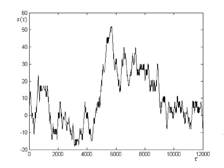
Figure 1: The graph of dependence of the system coordinates on time $x(\tau)$. The graph is plotted for the following parameters $x(0)=1.6,$ $p(0)=9.1,$ $S_{1}^{z}(0)=S_{2}^{z}=0.863,$ $U_{1}(0)=0.000081,$ $U_{2}(0)=0.000082,$ $\nu_{1}(0)=0.000083,$ $\nu_{2}(0)=0.000084,$ $g(0)=0.0000845,$ $f(0)=0.0000846$. As is seen from the plot trajectory has the chaotic form.

As is seen from Fig.1, the dynamics of the system even for zero detuning $\delta=0$ has chaotic form.

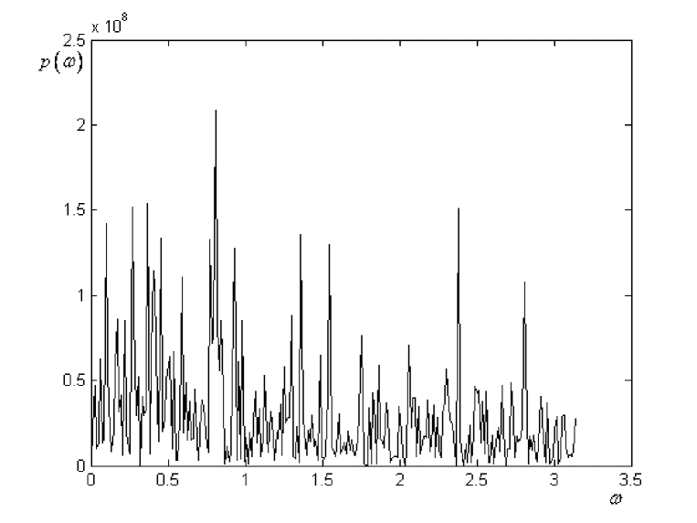
Figure 2: Fourier image of correlation function $G_{p}(\tau)=\langle P(t+\tau)P(t)\rangle$ ,$G_{p}(\omega)=\int d\tau exp(i\omega\tau)G_{p}(\tau)$. Finite width of correlation function confirms the existence of chaos. The graph is plotted for the same values of the parameters as for Fig.1.

The other parameters of the system have also chaotic spectrum (see Fig.3).

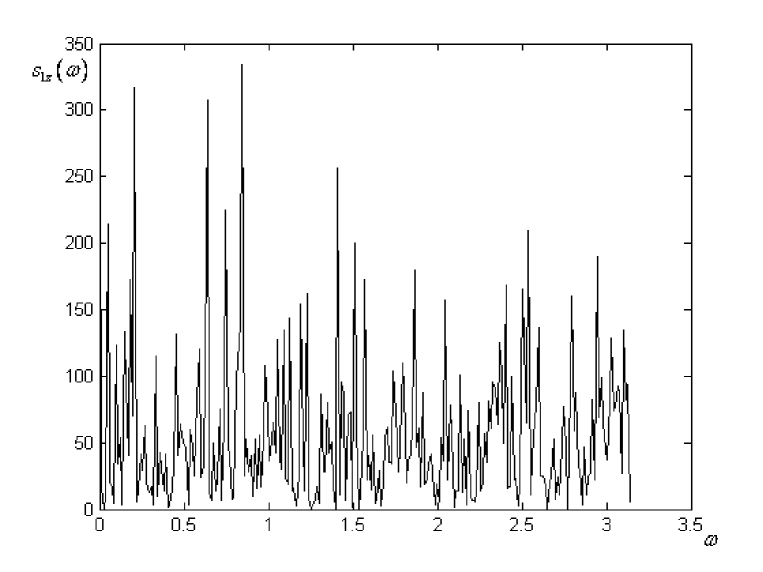
Figure 3: Fourier image of correlation function of variable $S_{1}^{z}$. The numerical vales of the parameters are analogous of that of Fig.1.

In order to be more convinced of dynamics to be chaotic, we have calculated even fractal dimension of the system.

In order to calculate fractal dimension of the system’s phase space we use the Grassberger-Procaccia algorithm Grassberger ; Procaccia . The idea of this algorithm is the following. Let us suppose, we obtain an ensemble of state vectors ${x_{i},~{}i=1,2,...N}$ by numerical solving of the set of equations, corresponding to successive steps of integration of differential equations. Choosing small parameter $\varepsilon$ we can use our result for evolution of the following sum:

$$C(\varepsilon)=\lim_{N\rightarrow\infty}\frac{1}{N(N-1)}\sum_{i,j=1}^{N}\theta(\varepsilon-|x_{i}-x_{j}|),$$ (12)

where $\theta$ is a step function

$$\theta(x)=\left\{\begin{array}[]{l}0\hskip 14.22636ptx<0\\ 1\hskip 14.22636ptx\geq 0\\ \end{array}\right.$$ (13)

According to Grassberger-Procaccia algorithm, if we know $C(\varepsilon)$, we can estimate strange attractor’s fractal dimension with the help of the following formula Grassberger ; Procaccia

$$D=\frac{C(\varepsilon)}{\lg(\varepsilon)}.$$ (14)

The numerical results are represented on Fig.4.

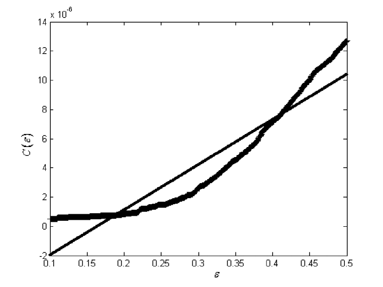
Figure 4: The graph of dependence of $C(\varepsilon)$ on $\varepsilon$ plotted using Grassberger-Proccacia algorithm for the values of the parameters analogous of that of Fig.1. A solid line corresponds to least-squares approximation of the results of date processing. The estimated fractal dimension is equal to $D=\frac{\ln(C(\varepsilon_{2}))-ln(C(\varepsilon_{1}))}{\ln\varepsilon_{2}-\ln\varepsilon_{1}}\approx 2.2$,$(\varepsilon_{1}\approx 0.12,\varepsilon_{2}\approx 0.41,C(\varepsilon_{1})\approx 0.5\cdot 10^{-6},C(\varepsilon_{2})\approx 7.5\cdot 10^{-6})$. The numerical data obtained verify that the dynamics of the system is chaotic. We shall make use of this fact in the second part of this work where quantum-statistical description will be used for the study of the systems dynamic without use of quasi-classical methods.

II. As we have shown in the first part of the work the dynamics of the system is chaotic for certain values of parameters even for zero detuning. When considering the state of the system with quantum-statistical methods we shall neglect kinetic energy of the system and operator $\hat{x}$ will be regarded as classical chaotic variable $x(t)$ , presented itself stochastic process. Condition of using this kind of approximation is the following: Acting on the system classical force is

$$|\overrightarrow{F}|=\frac{\Delta P}{\Delta t}=|\nabla_{x}\hat{H}_{SB}|\approx g_{0}K_{f}$$

So, classical momentum transferred to the atom is $\Delta P\approx\Delta tg_{0}K_{f}$. Then influence of the atomic motion on the energy levels can be neglected if $\frac{(\Delta P)^{2}}{2m}<|\hat{H}_{SB}|.$
This means $\frac{g_{0}K_{f}^{2}(\Delta t)^{2}}{2m}<1$.

Let us write Schrodinger equation of the system in interaction representation:

$$i\frac{d|\psi(t)>}{dt}=\hat{V}|\psi(t)>,$$ (15)

where

$$\hat{V}=\Omega(\hat{S}_{1}^{+}\hat{S}_{2}^{-}+\hat{S}_{1}^{-}\hat{S}_{2}^{+})+\omega_{f}\hat{b}^{+}\hat{b}-g_{0}\cos(k_{f}\hat{x})((\hat{S}_{1}^{+}+\hat{S}_{2}^{+})\hat{b}+(\hat{S}_{1}^{-}+\hat{S}_{2}^{-})\hat{b}^{+})$$ (16)

is an interaction operator.

Assume that at zero time $t=0$, the system’s wave function represents itself direct product of wave functions of atom $|\psi_{atom}>$ and $|\psi_{field}>$ field:

$$|\psi(t=0)>=|\psi_{atom}>\otimes|\psi_{field}>.$$

Here

$$|\psi_{atom}>=C_{00}|00>+C_{01}|01>+C_{10}|10>+C_{11}|11>,$$ (17)

$$|\psi_{field}>=\sum_{n}W_{n}|n>,$$ (18)

where $|n,m>$ is qubit’s wave function.

Because of interaction (16) the following transition between states are possible:

$$|0,0,n+1>\leftrightarrow|0,1,n>,~{}~{}|0,0,n+1>\leftrightarrow|1,0,n>,$$ (19)

$$|0,1,n>\leftrightarrow|1,1,n-1>,~{}~{}|1,0,n>\leftrightarrow|1,1,n-1>,~{}~{}|1,0,n>\leftrightarrow|0,1,n>.$$ (20)

The transition (19) correspond to the transitions between energy states with changing number of photons and the transitions (20) correspond to inter spin transitions. On the basis of equations (19),(20) we shall search for the solution of equation (15) in the following form:

$$|\psi(t)>=\sum_{n}C_{0,0,n+1}|0,0,n+1>+\sum_{n}C_{0,1,n}|0,1,n>+$$

$$+\sum_{n}C_{1,0,n}|1,0,n>+\sum_{n}C_{1,1,n-1}|1,1,n-1>.$$ (21)

Taking into account equations (15)-(21), we obtain the following equations for coefficients of resolution:

$$i\frac{dC_{0,0,n+1}}{dt}=\Omega C_{0,0,n+1}-g_{0}\cos(k_{f}x(t))\sqrt{n+1}(C_{1,0,n}+C_{0,1,n}),$$

$$i\frac{dC_{1,1,n-1}}{dt}=\Omega C_{1,1,n-1}-g_{0}\cos(k_{f}x(t))\sqrt{n}(C_{1,0,n}+C_{0,1,n}),$$

$$i\frac{dC_{0,1,n}}{dt}=\Omega C_{1,0,n}-g_{0}\cos(k_{f}x(t))(C_{1,1,n-1}\sqrt{n}+C_{0,0,n+1}\sqrt{n+1}),$$

$$i\frac{dC_{1,0,n}}{dt}=\Omega C_{0,1,n}-g_{0}\cos(k_{f}x(t))(C_{1,1,n-1}\sqrt{n}+C_{0,0,n+1}\sqrt{n+1}).$$ (22)

In the set of equations (22) let us pass to the new variables:

$$A(t)=C_{1,0,n}+C_{0,1,n},~{}~{}B(t)=\sqrt{n+1}C_{0,0,n+1}+\sqrt{n}C_{1,1,n-1}.$$ (23)

Taking into account (23), the set (22) takes the following form:

$$i\frac{dA(t)}{dt}=\Omega A(t)-2g_{0}\cos(k_{f}x(t))B(t),$$

$$i\frac{dB(t)}{dt}=\Omega B(t)-(2n+1)g_{0}\cos(k_{f}x(t))A(t).$$ (24)

If we introduce the new notations:

$$B^{\prime}(t)=\sqrt{2}B(t),~{}~{}A^{\prime}(t)=\sqrt{2n+1}A(t),~{}~{}\omega(t)=\sqrt{2}\sqrt{2n+1}g_{0}\cos(k_{f}x(t))$$ (25)

and after that:

$$C(t)=A^{\prime}(t)+B^{\prime}(t),~{}~{}D(t)=A^{\prime}(t)-B^{\prime}(t).$$ (26)

Taking into account equations (25) and (26), the set of equations (24) takes the simpler form:

$$i\frac{dC(t)}{dt}=\Omega C(t)-\omega(t)C(t),$$

$$i\frac{dD(t)}{dt}=\Omega D(t)+\omega(t)D(t).$$ (27)

It is readily seen that the solutions of the set (27) have the following form:

$$C(t)=C_{1}e^{i\Omega t}e^{i\int_{0}^{t}\omega(t^{\prime})dt^{\prime}},~{}~{}D(t)=C_{2}e^{i\Omega t}e^{-i\int_{0}^{t}\omega(t^{\prime})dt^{\prime}}.$$ (28)

Let us introduce the notations for the functionals:

$$Q[\omega(t)]=e^{i\int_{0}^{t}\omega(t^{\prime})dt^{\prime}},$$ (29)

$$Q^{\ast}[\omega(t)]=Q^{-1}[\omega(t)]=e^{-i\int_{0}^{t}\omega(t^{\prime})dt^{\prime}}.$$ (30)

Taking into account (27)-(30), the solutions of the set (24) takes the form:

$$A(t)=\frac{A^{\prime}(t)}{\sqrt{2n+1}}=\frac{C_{1}}{2\sqrt{2n+1}}e^{-i\Omega t}Q[\omega(t)]+\frac{C_{2}}{2\sqrt{2n+1}}e^{-i\Omega t}Q^{-1}[\omega(t)],$$ (31)

$$B(t)=\frac{B^{\prime}(t)}{\sqrt{2}}=\frac{C_{1}}{2\sqrt{2}}e^{-i\Omega t}Q[\omega(t)]-\frac{C_{2}}{2\sqrt{2}}e^{-i\Omega t}Q^{-1}[\omega(t)].$$ (32)

Taking into account (31), (32) and (23) we obtain:

$$C_{1,0,n}+C_{0,1,n}=\frac{C_{1}}{2\sqrt{2n+1}}e^{-i\Omega t}Q[\omega(t)]+\frac{C_{2}}{2\sqrt{2n+1}}e^{-i\Omega t}Q^{-1}[\omega(t)],$$ (33)

$$\sqrt{n+1}C_{0,0,n+1}+\sqrt{n}C_{1,1,n-1}=\frac{C_{1}}{2\sqrt{2}}e^{-i\Omega t}Q[\omega(t)]-\frac{C_{2}}{2\sqrt{2}}e^{-i\Omega t}Q^{-1}[\omega(t)].$$ (34)

The equations (33) and (34) are the conditions to determine time dependence of the coefficients of the functions (21). But for determination of four coefficients we need two more conditions. The third condition for determination of coefficients $C_{1,0,n}(t)$ and $C_{0,1,n}(t)$ is easily obtained from equation (22) and has the following form:

$$i\frac{d(C_{0,1,n}-C_{1,0,n})}{dt}=-\Omega(C_{0,1,n}-C_{1,0,n}).$$ (35)

From this we have:

$$C_{0,1,n}-C_{1,0,n}=C_{3}e^{i\Omega t}.$$ (36)

In order to obtain the last fourth condition, we introduce the notation:

$$\sqrt{n+1}C_{0,0,n+1}-\sqrt{n}C_{1,1,n-1}=F(t).$$ (37)

Then taking into account (22) we obtain for $F(t)$:

$$i\frac{dF(t)}{dt}=\Omega F(t)-g_{0}\cos(k_{f}x(t))A(t).$$ (38)

The solution (38) has the form:

$$F(t)=\frac{iC_{1}e^{-i\Omega t}}{2\sqrt{2}(2n+1)}\int\limits_{0}^{t}\omega(t^{\prime})Q[\omega(t^{\prime})]dt^{\prime}+$$

$$+\frac{iC_{2}e^{-i\Omega t}}{2\sqrt{2}(2n+1)}\int\limits_{0}^{t}\omega(t^{\prime})Q^{-1}[\omega(t^{\prime})]dt^{\prime}+C_{4}e^{-i\Omega t}.$$ (39)

For further simplification of equation (39) consider the expression:

$$\int\limits_{0}^{t}\omega(t^{\prime})Q[\omega(t^{\prime})]dt^{\prime}=\int\limits_{0}^{t}\omega(t^{\prime})e^{i\int\limits_{0}^{t^{\prime}}\omega(t^{\prime\prime})dt^{\prime\prime}}dt^{\prime}$$ (40)

and let us introduce the notation:

$$\Omega_{0}(t^{\prime})=\int\limits_{0}^{t^{\prime}}\omega(t^{\prime\prime})dt^{\prime\prime}.$$ (41)

Then it is readily seen that:

$$\int\limits_{0}^{t}\omega(t^{\prime})Q[\omega(t^{\prime})]dt^{\prime}=\int\limits_{0}^{t}d\Omega_{0}(t^{\prime})e^{i\Omega_{0}(t^{\prime})}=-i(e^{i\Omega_{0}(t)}-1).$$ (42)

By analogy with previous one:

$$\int\limits_{0}^{t}\omega(t^{\prime})Q^{-1}[\omega(t^{\prime})]dt^{\prime}=\int\limits_{0}^{t}d\Omega_{0}(t^{\prime})e^{-i\Omega_{0}(t^{\prime})}=i(e^{-i\Omega_{0}(t)}-1).$$ (43)

Taking into account (42), (43), the expression (39) takes the form:

$$F(t)=\frac{C_{1}e^{-i\Omega t}}{2\sqrt{2}(2n+1)}(Q[\omega(t)]-1)-\frac{C_{2}e^{-i\Omega t}}{2\sqrt{2}(2n+1)}(Q^{-1}[\omega(t)]-1)+C_{n}e^{-i\Omega t}.$$ (44)

Taking into consideration (33), (34),(36) and (44) we can yet write down the set of four algebraic equations for the coefficients of wave function (21):

$$C_{1,0,n}+C_{0,1,n}=\frac{C_{1}}{2\sqrt{2n+1}}e^{-i\Omega t}Q[\omega(t)]+\frac{C_{2}}{2\sqrt{2n+1}}e^{-i\Omega t}Q^{-1}[\omega(t)],$$

$$\sqrt{n+1}C_{0,0,n+1}+\sqrt{n}C_{1,1,n-1}=\frac{C_{1}}{2\sqrt{2}}e^{-i\Omega t}Q[\omega(t)]-\frac{C_{2}}{2\sqrt{2}}e^{-i\Omega t}Q^{-1}[\omega(t)],$$

$$C_{0,1,n}-C_{1,0,n}=C_{3}e^{i\Omega t},$$

$$\sqrt{n+1}C_{0,0,n+1}-\sqrt{n}C_{1,1,n-1}=$$

$$=\frac{C_{1}e^{i\Omega t}}{2\sqrt{2}(2n+1)}(Q[\omega(t)]-1)-\frac{C_{2}e^{-i\Omega t}}{2\sqrt{2}(2n+1)}(Q^{-1}[\omega(t)]-1)+C_{4}e^{-i\Omega t}.$$ (45)

Here the coefficients of integration are connected with the initial conditions via the relations:

$$C_{1}=\sqrt{2n+1}(C_{0,1,n}(0)+C_{1,0,n}(0))+\sqrt{2}(\sqrt{n+1}C_{0,0,n+1}(0)+\sqrt{n}C_{1,1,n-1}(0)),$$

$$C_{2}=\sqrt{2n+1}(C_{0,1,n}(0)+C_{1,0,n}(0))-\sqrt{2}(\sqrt{n+1}C_{0,0,n+1}(0)+\sqrt{n}C_{1,1,n-1}(0)),$$

$$C_{3}=C_{0,1,n}-C_{1,0,n},$$

$$C_{4}=C_{0,0,n+1}\sqrt{n+1}-C_{1,1,n-1}\sqrt{n}.$$ (46)

by solving the set of equations (45), it is possible to determine time dependence of wave function (21) and by means of this to determine quantum state of qubit:

$$C_{0,0,n+1}(t)=\frac{C_{1}e^{-i\Omega t}\sqrt{n+1}}{2\sqrt{2}(2n+1)}Q[\omega(t)]-\frac{C_{2}e^{-i\Omega t}\sqrt{n+1}}{2\sqrt{2}(2n+1)}Q^{-1}[\omega(t)]+$$

$$+(\frac{C_{4}}{2\sqrt{n+1}}-\frac{C_{1}}{4\sqrt{2}\sqrt{n+1}(2n+1)}+\frac{C_{2}}{4\sqrt{2}\sqrt{n+1}(2n+1)})e^{-i\Omega t},$$

$$C_{1,1,n-1}(t)=\frac{C_{1}e^{-i\Omega t}}{2\sqrt{2}}\frac{\sqrt{n}}{(2n+1)}Q[\omega(t)]-\frac{C_{2}e^{-i\Omega t}}{2\sqrt{2}}\frac{\sqrt{n}}{(2n+1)}Q^{-1}[\omega(t)]+$$

$$+(-\frac{C_{4}}{2\sqrt{n+1}}+\frac{C_{1}}{4\sqrt{2}\sqrt{n+1}(2n+1)}-\frac{C_{2}}{4\sqrt{2}\sqrt{n+1}(2n+1)})e^{-i\Omega t},$$

$$C_{1,0,n}(t)=\frac{C_{1}}{4\sqrt{2n+1}}e^{-i\Omega t}Q[\omega(t)]+\frac{C_{2}}{4\sqrt{2n+1}}e^{-i\Omega t}Q^{-1}[\omega(t)]+\frac{C_{3}}{2}e^{i\Omega t},$$

$$C_{0,1,n}(t)=\frac{C_{1}}{4\sqrt{2n+1}}e^{-i\Omega t}Q[\omega(t)]+\frac{C_{2}}{4\sqrt{2n+1}}e^{-i\Omega t}Q^{-1}[\omega(t)]-\frac{C_{3}}{2}e^{i\Omega t}.$$ (47)

As is seen from (47), time dependence of the coefficients of wave function (21) describing quantum state of qubit is determined by the functional:

$$Q[\omega(t)]=e^{i\int_{0}^{t}\omega(t^{\prime})dt^{\prime}},$$ (48)

where

$$\omega(t)=\sqrt{2(2n+1)}g_{0}\cos(k_{f}x(t)).$$ (49)

As is seen from (49) time dependence of quantum state depends on $x(t)$. Thus in order to determine qubit’s state, it is necessary to know the coordinate of the, system as explicit function of time $x(t)$. But on the other hand as we have showed in the first part of the work, because of the dynamics to be chaotic $x(t)$ may be considered as classical chaotic process. In this case for determination of the system’s state it is necessary to average the functional (48) by all realizations of stochastic variable $x(t)$. For this, we represent stochastic average of functional (48) in the form of the following continual integral:

$$<Q[\omega(t)]>=<exp(i\int_{0}^{t}\omega(t^{\prime})dt^{\prime})>=\lim\limits_{N\rightarrow\infty\atop\Delta t_{k}\rightarrow 0}\int d\omega_{N}\ldots d\omega_{1}exp(i\sum_{k=i}^{N}\omega_{k}\Delta t_{k})P_{N}(\omega),$$ (50)

where

$$P_{N}(\omega)=(2\pi)^{-N}\int d\lambda_{1}\ldots d\lambda_{N}exp[-i\sum_{k=i}^{N}\lambda_{k}\omega_{k}]exp[-\frac{1}{2}\sum_{kk^{\prime}}C_{kk^{\prime}}\lambda_{k}\lambda_{k^{\prime}}]$$ (51)

is Fourier image of distribution function, $\Delta t_{k}=t^{(k)}-t^{(k-1)},~{}t^{(0)}=0,~{}t^{(N)}=t.$

It is readily seen that by taking into account (51), the expression (50) can be rewritten in the following form:

$$\int d\omega_{N}\ldots d\omega_{1}exp(i\sum_{k=1}^{N}\omega_{k}\Delta t_{k})P_{N}(\omega)=$$

$$=\int d\lambda_{1}\ldots d\lambda_{N}exp[-\frac{1}{2}\sum_{kk^{\prime}}C_{kk^{\prime}}\lambda_{k}\lambda_{k^{\prime}}]\prod_{k=1}^{N}\frac{1}{2\pi}\int exp[i\omega_{k}(\Delta t_{k}-\lambda_{k})]=$$

$$=\int d\lambda_{1}\ldots d\lambda_{k}\delta(\lambda_{1}-\Delta t_{1})\delta(\lambda_{2}-\Delta t_{2})\ldots\delta(\lambda_{N}-\Delta t_{N})exp[-\frac{1}{2}\sum_{kk^{\prime}}C_{kk^{\prime}}\lambda_{k}\lambda_{k^{\prime}}].$$ (52)

Taking into account (52) for statistically averaged functional we obtain:

$$<Q[\omega(t)]>=\lim_{N\rightarrow\infty}exp[-\frac{1}{2}\sum_{kk^{\prime}}C(t^{(k)},t^{(k^{\prime})})\Delta t^{k}\Delta t^{k^{\prime}}]=$$

$$=exp(-\frac{1}{2}\int\limits_{0}^{t}dt^{\prime}\int\limits_{0}^{t}dt^{\prime\prime}C(t^{\prime},t^{\prime\prime})).$$ (53)

For random processes $C(t^{\prime},t^{\prime\prime})=C(t^{\prime}-t^{\prime\prime})$. Then introducing the new variables: $t^{\prime}-t^{\prime\prime}=\tau$, $t^{\prime}+t^{\prime\prime}=\xi$, and assuming that correlation function has Gaussian form
$C(\tau)=<\omega(t+\tau)\omega(\tau)>=e^{-\alpha_{0}\tau^{2}}$, finally from (53) we obtain:

$$<Q[\omega(t)]>=exp[-\frac{t}{2}\sqrt{\frac{\pi}{\alpha_{0}}}Erf(t\sqrt{\alpha_{0}})],$$ (54)

where $Erf(\ldots)$ is error function Handbook .

Assume that at zero time the system was in the state:

$$|\psi(0)>=|\psi_{atom}>\otimes|\psi_{field}>,$$ (55)

where

$$|\psi_{field}>=\sum_{n}W_{n}|n>.$$ (56)

Comparing (55), (56) with:

$$|\psi(0)>=\sum_{n}C_{0,0,n+1}(0)|0,0,n+1>+\sum_{n}C_{0,1,n}(0)|0,0,n>+$$

$$+\sum_{n}C_{1,0,n}(0)|1,0,n>+\sum_{n}C_{1,1,n-1}(0)|1,1,n-1>$$ (57)

it is possible to obtain the following relations for the initial conditions:

$$C_{00}W_{n+1}=C_{00n+1}(0),~{}~{}C_{01}W_{n}=C_{01n}(0),$$

$$C_{10}W_{n}=C_{10n}(0),~{}~{}C_{00}W_{n+1}=C_{00n+1}(0).$$ (58)

Let us determine the values measured on experiment that are connected with population difference of levels:

$$I_{11,01}=W(t,|11>)-W(t,|01>),$$

$$I_{11,10}=W(t,|11>)-W(t,|10>),$$

$$I_{10,00}=W(t,|10>)-W(t,|00>),$$

$$I_{01,00}=W(t,|01>)-W(t,|00>),$$

$$I_{11,00}=W(t,|11>)-W(t,|00>)=\frac{1}{2}(I_{11,01}+I_{11,10})+\frac{1}{2}(I_{01,00}+I_{01,00}),$$ (59)

where

$$W(t,|11>)=\sum_{n=0}^{\infty}|C_{1,1,n-1}(t)|^{2},$$

$$W(t,|01>)=\sum_{n=0}^{\infty}|C_{0,1,n}(t)|^{2},$$

$$W(t,|10>)=\sum_{n=0}^{\infty}|C_{1,0,n}(t)|^{2},$$

$$W(t,|00>)=\sum_{n=0}^{\infty}|C_{0,0,n+1}(t)|^{2}.$$ (60)

For illustration let us calculate for example $W(t,|1,0>)$. Taking into account (47) and (54) we obtain:

$$<W(t,|10>)>=\frac{1}{8}\sum_{n=0}^{\infty}(C_{10}W_{n}+C_{01}W_{n})^{2}+\frac{1}{4}\sum_{n=0}^{\infty}\frac{1}{2n+1}(\sqrt{n+1}C_{0,0}W_{n+1}+$$

$$+\sqrt{n}C_{1,1}W_{n-1})^{2}+\frac{1}{4}\sum_{n=0}^{\infty}(C_{1,0}W_{n}-C_{0,1}W_{n})^{2}+<W(t,|10>)>_{int},$$ (61)

where $<W(t,|1,0>)>_{int}$ denote interference terms whose explicit forms are not brought here for the sake of brevity. The point is that interference terms contain terms of the following form:

$$<Q^{-2}[\omega(t)]>,~{}~{}<Q^{2}[\omega(t)]>,~{}~{}<e^{2i\Omega t}Q^{-1}[\omega(t)]>.$$ (62)

These quantities, as well as (54), fall down quickly after the lapse of time. For example:

$$<e^{2i\Omega t}Q^{-1}[\omega(t)]>=e^{2i\Omega t}exp(-\frac{t}{2}\sqrt{\frac{\pi}{\alpha_{0}}}Erf(t\sqrt{\alpha_{0}})).$$ (63)

As is seen from (63), for time interval that is more then the time of correlation function of the random quantity $\omega(t)$ (49), $t>\sqrt{\frac{\pi}{\alpha_{0}}}$

$$C(\tau)=<\omega(t+\tau)\omega(\tau)>=e^{-\alpha_{0}\tau^{2}}$$ (64)

interferentional terms can be neglected in (61). Situation is analogous for other quantities as well from (59),(60). Thus we were able to prove that because of dynamics to be chaotic zeroing of interferentional terms occurs. This fact of zeroing of inerferentional terms has deep physical sense. This means that the system execute transition from pure quantum-mechanical state to mixed one Landau . Such a transition is irreversible, as information about the phase of the system is lost. Transition from pure quantum state to mixed one is one of the manifestations of quantum chaos Ugulava ; Chotorlishvili ; Nickoladze ; Gvarjaladze ; Skrinnikov . Formulae analogous to (61) can be obtained for other quantities (60) as well:

$$<W(t,|0,0>)>=\sum_{n=0}^{\infty}\frac{n+1}{4(2n+1)}(C_{10}W_{n}+C_{01}W_{n})^{2}+\frac{1}{2}\sum_{n=0}^{\infty}\frac{n+1}{(2n+1)^{2}}(\sqrt{n+1}C_{0,0}W_{n+1}+$$

$$+\sqrt{n}C_{1,1}W_{n-1})^{2}+\sum_{n=0}^{\infty}\frac{n}{(2n+1)^{2}}(\sqrt{n}C_{0,0}W_{n+1}-\sqrt{n+1}C_{1,1}W_{n-1})^{2}$$

$$<W(t,|11>)>=\sum_{n=0}^{\infty}\frac{n}{4(2n+1)}(C_{10}W_{n}+C_{01}W_{n})^{2}+\frac{1}{2}\sum_{n=0}^{\infty}\frac{n}{(2n+1)^{2}}(\sqrt{n+1}C_{0,0}W_{n+1}+$$

$$+\sqrt{n}C_{1,1}W_{n-1})^{2}+\sum_{n=0}^{\infty}\frac{n+1}{(2n+1)^{2}}(\sqrt{n}C_{0,0}W_{n+1}-\sqrt{n+1}C_{1,1}W_{n-1})^{2}$$

$$<W(t,|10>)>=<W(t,|0,1>)>=\frac{1}{8}\sum_{n=0}^{\infty}(C_{10}W_{n}+C_{01}W_{n})^{2}+$$

$$+\frac{1}{4}\sum_{n=0}^{\infty}\frac{1}{2n+1}(\sqrt{n+1}C_{0,0}W_{n+1}+\sqrt{n}C_{1,1}W_{n-1})^{2}+\frac{1}{4}\sum_{n=0}^{\infty}(C_{10}W_{n}-C_{01}W_{n})^{2}$$ (65)

where $C_{00},~{}C_{01},~{}C_{10},~{}C_{11}$ quantities are populations of corresponding levels, $W_{n}$ describes state of the field. It is usually assumed that $W_{n}$ satisfy Gaussian distribution Schleich :

$$W_{n}=\frac{1}{\sqrt{2\pi\Delta n^{2}}}exp[-\frac{(n-\bar{n})^{2}}{\Delta n^{2}}].$$ (66)

As we noted above transition from pure state to mixed one is irreversible. In order this fact to be confirmed, let us calculate change of the system’s entropy.

Let us assume, that the system at zero time was in state $C_{00,n+1}$ . In this case the system’s entropy according to Ropke , Fujita is:

$$S(t=0)=-\sum_{i=1}^{4}\rho_{i}\ln\rho_{i}=0,$$ (67)

as only one of the elements of density matrix $\rho$ is nonzero:

$$\rho_{1}(t=0)=|C_{00,n+1}(0)|^{2}=1,~{}~{}\rho_{2}(t=0)=\rho_{3}(t=0)=\rho_{4}(t=0)=0.$$ (68)

After the lapse of time that is more than the time of transition between the levels $t_{0}\sim 1/g_{0},t>t_{0}$ the system has time to execute transition between levels. That is why probability to find system in other states will be nonzero:

$$C_{11}\neq 0,~{}~{}C_{01}\neq 0,~{}~{}C_{10}\neq 0~{}~{}~{}~{}~{}t>t_{0}.$$ (69)

Despite of this fact to talk about probability of population of different states is early yet. The point is that in time interval:

$$t_{0}<t<\sqrt{\frac{\pi}{\alpha_{0}}}$$ (70)

interferentional terms in equations (61),(65) are nonzero. Therefore the state of the system will be pure one. But unlike of the initial state (68),which is simple state, the state of the system in time interval (70) is superposition one.

Superposition state is pure quantum mechanical state and only after zeroing of interferentional terms in (61) and (65) superposition state passes to mixed one. Such a transition occurs in times:

$$t>\sqrt{\frac{\pi}{\alpha_{0}}}$$ (71)

But in time interval (70) while the system is in pure superposition state, from the symmetry point of view, it is clear that the coefficient values(69) have to satisfy the following relation:

$$C_{00}\left(t_{0}<t<\sqrt{\frac{\pi}{\alpha}}\right)\sim C_{11}\left(t_{0}<t<\sqrt{\frac{\pi}{\alpha}}\right)\sim$$

$$\sim C_{01}\left(t_{0}<t<\sqrt{\frac{\pi}{\alpha}}\right)\sim C_{10}\left(t_{0}<t<\sqrt{\frac{\pi}{\alpha}}\right)\sim C.$$ (72)

Taking into account normalization condition:

$$\sum_{i,j=0}^{1}<W(t,|ij>)>=1$$ (73)

and (72), from (65)we obtain:

$$C^{2}(\sum_{n=0}^{\infty}(W_{n}^{2}+W_{n+1}^{2}+W_{n-1}^{2}))=1.$$ (74)

Then taking into account the relation:

$$<W(t,|0,1>)>=<W(t,|1,0>)>$$ (75)

it is easy to obtain the condition from (65):

$$<W(t,|11>)>+<W(t,|00>)>=<W(t,|01>)>+<W(t,|10>)>+$$

$$(+\sum_{n=0}^{\infty}\frac{n}{(2n+1)}(\sqrt{n}C_{00}W_{n+1}-\sqrt{n+1}C_{11}W_{n-1})^{2}.$$ (76)

The condition (76) means in its turn that at times (71) mixed states are formed in the system in which the levels:

$$\rho_{1}=<W(t>\sqrt{\pi/\alpha}|11>)>=a,~{}~{}\rho_{2}=<W(t>\sqrt{\pi/\alpha}|00>)>=b$$ (77)

are populated with more probability than the levels:

$$\rho_{3}=<W(t>\sqrt{\pi/\alpha}|01>)>=\rho_{4}=<W(t>\sqrt{\pi/\alpha}|10>)>=c,$$ (78)

where quantities $a,b,c$ satisfy normalization condition:

$$Tr(\hat{\rho})=a+b+2c=1,~{}~{}a+b>2c$$ (79)

Taking into account (67), (77), (78) and (79) it is easy to see that during evolution of the system from pure quantum-mechanical state (68) to mixed one (77), (78) increase of entropy occurs.

$$\Delta S=S(t>\sqrt{\pi/\alpha})-S(t=0)=-(a\ln a+b\ln b+2c\ln c)>0,$$

$$0<a<1,~{}~{}0<b<1,~{}~{}0<c<1$$ (80)

III Conclusion

Let sum up and analyze the results obtained in conclusion.

The aim of this work was to study two 1/2 spin qubit system being subject to resonator field. Interest to such a systems is caused by the fact that they are the most perspective to be used in quantum computer. The question that came up is the following: by how much will be state of the system controllable and dynamics reversible? We have considered the most general case, when interaction of the system with field depends on coordinate of the system inside resonator.

Contrary to generally accepted opinion, it has turned out that the absence of detuning between resonator field and frequency of the system does not guarantee reversibility of the system’s state. During evolution in time the system executes irreversible transition from pure quantum-mechanical state to mixed one. At the same time, the time needed for formation of mixed state $t>\sqrt{\pi/\alpha_{0}}$ is determined completely by the system’s parameters $\alpha=\frac{K_{f}^{2}}{mg_{0}}$.

One more peculiarity of the problem studied is the following. It is well known Buchleitner ; Saif ; Farhan ; Perel'man ; Leichtle ; Averbukh that for integrable quantum systems complete and fractional quantum revivals are typical Buchleitner ; Saif ; Farhan ; Perel'man ; Leichtle ; Averbukh . In our case because of dynamics to be chaotic phase incursion occurs. This results in zeroing of interferentional terms and irreversible losing of information about the system’s state. This guaranties the absence of quantum revivals for our system. the noted fact may be especially interesting for experimental investigation of the system under consideration.

References

(1) T. Aoki et al. Nature 443, 671 (2006).
(2) H. Mabuchi and A. Doherty, Science 298, 1372 (2002).
(3) C.J. Hood et al., Science 287, 1447 (2000).
(4) J.Raimond, M.Brune, and S.Haroche, Rev.Mod.Phys. 73, 565 (2001).
(5) Q.A. Tuchette et al.,
Phys.Rev.Lett. 75, 4710 (1995).
(6) D.J. Wineland et al.,
J.Res.Nat.Inst.Stand.Technol. 103, 259 (1998).
(7) P. Schleich, Quantum Optics in Phase Space, Wiley. VCH,
Berlin (2001).
(8) H. Fujisaki, T. Miyadera, and A. Tanaka, Phys.Rev.E
67, 066201 (2003).
(9) A.J. Scott and C.M. Caves, J.Phys. A 36, 9553 (2003).
(10) M. Novaes and Marcus A.M. de Aguiar, Phys.Rev E
70,045201(R)(2004).
(11) Q. Xie and W. Hai, Eur.Phys.J. 33D, 265 (2005).
(12) R.M. Angelo, K. Furuya, M.C. Nemes, and G.Q. Rellegrino, Phys.Rev.A
64, 043801 (2001).
(13) J. Ye, D.W. Yemooy, and H.J.
Kimble, Phys.Rev.Lett. 83, 4987 (1999).
(14) S.J. van Enk, J. McKeever, H.J. Kimble, and J. Ye, Phys.Rev.A.
64, 013407(2001).
(15) P.M. Punstermann, T. Fischer, P. Maunz,
P.W.H. Pinkse, and G. Rempe, Phys.Rev.Lett. 82, 379
(1999).
(16) D. Loss
and D.P. DiVincenzo, Phys.Rev. A 57, 120 (1998.)
(17) B.E. Kane, Nature 393, 133 (1998).
(18) A.J. Skinner, M.E. Davenport, and B.E. Kane
Phys.Rev.Lett. 90, 087901 (2003).
(19) T.D. Ladd, J.R. Goldman, F. Yamaguchi, Y. Yamamoto, E. Abe, and
K.M.Itoh, Phys.Rev.Lett. 89, 017901 (2002).
(20) R. de Sousa, J.D. Delgado, and S. Das Sarma, Phys.Rev. A
70, 052304(2004).
(21) Xiao-Zhong Yuan, Hsi-Sheng Goan, and Ka-Di Zhu, Phys.Rev. B 75, 045331
(2007).
(22) S. Prants, N. Edelman, and G. Zaslavsky, Phys.Rev. E
66, 046222 (2002).
(25) P. Grassberger and I. Procaccia, Physica
D,9, 189 (1983).
(26) Handbook of Mathematical Functions with Formulas, Graphs, and Mathematical Tables National Bureau of Standards,
Applied Mathematical Series, 55, U.S. Government Printing,
(Washington D.C., 1964).
(27) L.D. Landau and E.M. Lifschitz,
Statistical Mechanics, v.5, (in Russian) (Nauka Moscow 1976).
(28) A. Ugulava, L. Chotorlishvili, and K. Nickoladze, Phys.Rev. E
68, 026216 (2003).
(29) A. Ugulava, L. Chotorlishvili, and K. Nickoladze, Phys.Rev. E
70, 026219 (2004).
(30) A. Ugulava, L. Chotorlishvili, and K. Nickoladze, Phys.Rev. E
71, 056211 (2005).
(31) A. Ugulava, L.Chotorlishvili, T. Gvarjaladze, and S.Chkhaidze,
Mod.Phys. Lett. B, 21, 415 (2007).
(32) L. Chotorlishvili, A. Ugulava, T. Kereselidze, V. Skrinnikov,
Mod.Phys.Lett.B 21, 79 (2007).
(33) G. Ropke, Statistische Mechanik fur das Nichtgleichgewicht VEB Deutscher Verlag der
Wissenschaften, Berlin (1987).
(34) S. Fujita, Introduction to Non-Equilibrium Quantum Statistical Mechanics W.B.Saunders
Company, Philadelphia-London (1966).