Low accretion rates at the AGN cosmic downsizing epoch

Abstract

Context. X-ray surveys of Active Galactic Nuclei (AGN) indicate “cosmic downsizing”, with the comoving number density of high-luminosity objects peaking at higher redshifts ($z\sim 2$) than low-luminosity AGN ($z<1$).

Aims. We test whether downsizing is caused by activity shifting towards low-mass black holes accreting at near-Eddington rates, or by a change in the average rate of accretion onto supermassive black holes. We estimate the black hole masses and Eddington ratios of an X-ray selected sample of AGN in the Chandra Deep Field South at $z<1$, probing the epoch where AGN cosmic downsizing has been reported.

Methods. Black hole masses are estimated both from host galaxy stellar masses, which are estimated from fitting to published optical and near-infrared photometry, and from near-infrared luminosities, applying established correlations between black hole mass and host galaxy properties. Both methods give consistent results. Comparison and calibration of possible redshift-dependent effects is also made using published faint host galaxy velocity dispersion measurements.

Results. The Eddington ratios in our sample span the range $\sim 10^{-5}-1$, with median $\log\left(L_{\mathrm{bol}}/L_{\mathrm{Edd}}\right)=-2.87$, and with typical black hole masses $M_{\mathrm{BH}}\sim 10^{8}$ M_⊙. The broad distribution of Eddington ratios is consistent with that expected for AGN samples at low and moderate luminosity. We find no evidence that the CDF-S AGN population is dominated by low-mass black holes accreting at near-Eddington ratios and the results suggest that diminishing accretion rates onto average-sized black holes are responsible for the reported AGN downsizing at redshifts below unity.

1 Introduction

One of the most significant recent discoveries in studying the cosmological evolution of AGN has been the discovery that lower-luminosity AGN ($L_{2-10\,\mathrm{keV}}\sim 10^{41}-10^{43}$ erg s^-1) peak in their comoving space density at lower redshift, $z\la 1$, than higher-luminosity AGN ($L_{2-10\,\mathrm{keV}}\sim 10^{45}-10^{47}$ erg s^-1), which peak at $z\sim 2$ (Cowie et al. 2003; Steffen et al. 2003; Ueda et al. 2003; Barger et al. 2005; Giacconi et al. 2002; La Franca et al. 2005; Hasinger et al. 2005; Hopkins et al. 2007).

The implication of the phenomenon for black hole growth can be seen from the emissivity of AGN in different luminosity ranges (Hasinger et al. 2005, Fig. 5b): at redshifts $z\gtrsim 2$ the major contribution to the total emissivity comes from high luminosity AGN ($L_{0.5-2\,\mathrm{keV}}\sim 10^{44}-10^{45}\,$erg s^-1), while at $z\sim 0$ the major contribution shifts to lower luminosities ($L_{0.5-2\,\mathrm{keV}}\sim 10^{43}-10^{44}\,$erg s^-1), with a significant contribution from low luminosity AGN ($L_{0.5-2\,\mathrm{keV}}\sim 10^{42}-10^{43}\,$erg s^-1). If we simply relate the emissivity to the accretion rate onto black holes, it follows that a significant contribution to the black hole growth has shifted from high luminosity objects at high redshifts to low luminosity ones at low redshifts. This shift has been named ‘AGN cosmic downsizing’, by analogy with the phenomenon observed in the cosmic star formation rate density in normal galaxies (‘cosmic downsizing’, e.g. Cowie et al. 1996; Bauer et al. 2005; Panter et al. 2007). There, the decline in star formation rate at redshifts below $z\lesssim 2$ has been shown to be due to star formation preferentially stopping in high mass galaxies towards the present day, and the major contribution to the star formation density at $z\sim 0$ arises from low mass systems. The relationship of galaxy downsizing to AGN downsizing is unclear: the phenomenon in AGN is observed in luminosity, and so an interpretation of the phenomenon as being downsizing in the mass of active black holes requires either an assumption of the relationship between AGN luminosity and black hole mass as a function of redshift or measurement of that relationship. Supporting evidence that low-luminosity AGN at low redshift are preferentially powered by black holes with lower masses than the typical distribution of local black holes has been found when using [OIII] emission as a measure of activity (Heckman et al. 2004), although when radio activity is measured instead, higher-mass black holes seem more active locally (Best et al. 2005).

In this paper we present a determination of the distribution of Eddington ratios for an X-ray selected sample of AGN in the CDF-S, at $z<1$. This redshift range is of particular interest, as it is the epoch in which the total AGN emissivity is dominated by moderate and low luminosity AGN — the AGN downsizing epoch. The Eddington ratios are found by first estimating black hole masses from photometrically-estimated stellar masses and luminosities. These black holes masses are then compared with the host galaxy velocity dispersions from van der Wel et al. (2005). The Eddington ratio is then calculated as $\lambda\equiv L_{\rm bol}/L_{\rm Edd}$ where $L_{\rm bol}$ is the AGN bolometric luminosity inferred from the observed X-ray luminosity and $L_{\rm Edd}$ is the Eddington luminosity. We assume $H_{0}=71$ km s^-1 Mpc^-1, $\Omega_{M}=0.3$ and $\Omega_{\Lambda}=0.7$ throughout.

2 The AGN sample

The CDF-S has been the subject of a 1 Ms Chandra observation reaching a flux limit of $4.5\times 10^{-16}\,$erg cm^-2 s^-1 in the 2–10 keV band (Rosati et al. 2002). At redshift $z=1$ the flux limit corresponds to a hard X-ray luminosity of $L_{2-10\,\mathrm{keV}}=10^{42.4}$ erg s^-1, meaning that the AGN population that dominates the downsizing, with $L_{2-10\,\mathrm{keV}}\sim 10^{41.5}-10^{43.5}$ erg s^-1 at $z<1$, is observed in the survey. Optical imaging and identifications have been published by Giacconi et al. (2002) with optical spectroscopic follow-up by Szokoly et al. (2004, hereafter S04), providing spectroscopic redshifts, in addition to X-ray and optical classifications. The total number of X-ray sources in the catalogue is 347, of which 251 are detected in the hard X-ray band. Availability of the spectroscopic (S04) and photometric redshifts (Zheng et al. 2004; Mainieri et al. 2005) together with the deep X-ray exposure has allowed the X-ray spectroscopic analysis published by Tozzi et al. (2006). For bright sources, these authors fitted the photon spectral index $\Gamma$ and the absorbing hydrogen column density $N_{\mathrm{H}}$ simultaneously, while for fainter sources the photon spectral index was fixed at the mean value $\langle\Gamma\rangle=1.8$. The $N_{\mathrm{H}}$ distribution was found to have a log-normal shape, peaking at $\log(N_{\mathrm{H}}/\mathrm{cm}^{-2})=23.1$. From the fitted spectra, absorption-corrected X-ray luminosities were estimated and have been made publicly available by Tozzi et al.. There are 321 objects classified by their absorption-corrected total X-ray luminosity as AGN ($L_{X}>10^{41}$ erg s^-1), and the completeness of the spectroscopic (X-ray) catalogue with respect to the photometric one is $\sim 99\%$.

Deep BVIz optical photometry in CDF-S is provided by the GOODS survey, from ACS/HST imaging (Giavalisco et al. 2004) with sensitivity limits 27.8, 27.8, 27.1, 26.6 (AB magnitudes, 10$\sigma$ limits, in $0\aas@@fstack{\prime\prime}2$ aperture). The deepest R-band data available (R${}_{AB}\sim 26.7$) are included in the 1 Ms catalogue (Giacconi et al. 2002). In the near-infrared (NIR), Olsen et al. (2006) have re-reduced the ESO Imaging Survey data (Arnouts et al. 2001), with the observations reaching median limiting magnitudes J${}_{AB}\sim 23.1$, K${}_{AB}\sim 22.2$ ($5\sigma$ limits, in $2^{\prime\prime}$ aperture). In the infrared, the Spitzer Wide-area InfraRed Extragalactic survey (SWIRE) provides observations in four IRAC bands: 3.6, 4.5, 5.8, 8.0$\,\mu$m (Surace et al. 2005). The 90% completeness limits for SWIRE Data Release 2 are $m_{AB}=(21.0,20.96,19.84,19.53)$. CDF-S is also one of the fields covered by the COMBO-17 survey, with photometry in 12 medium-band and 5 broad-band filters (Wolf et al. 2004). The COMBO-17 magnitude limits are 24.7, 25.0, 24.5, 25.6, 23.0 in U, B, V, R, I bands respectively (AB magnitudes, $10\sigma$ limits, $\sim 1\aas@@fstack{\prime\prime}5$ aperture), while limiting magnitudes in the 12 medium-band filters are in the range $m_{AB}=22.0-23.9$.

Recently the deepest CDF-S optical to infrared public data has been compiled into a uniform photometric catalogue of NIR-selected objects by the GOODS-MUSIC (MUltiwavelength Southern Infrared Catalog) project (Grazian et al. 2006). The catalogue is based on imaging in BVIz from ACS/HST, JHK_s from ISAAC/VLT, U band from the 2.2ESO and VLT-VIMOS, and 4 IRAC/Spitzer bands. The authors have developed a ‘PSF-matching’ (point spread function) algorithm, which allows finding precise object colours between ground-based and space-based images.

In this paper we define and analyse two samples drawn from the above data. We limit the redshift to $z<1$, as we are interested in probing the epoch for which AGN downsizing has been reported (Barger et al. 2005). Given the X-ray survey flux limits, we are guaranteed to probe the AGN population predominantly responsible for the inferred downsizing. We include all $z<1$ objects X-ray classified as AGN ($L_{X}>10^{41}\,\mathrm{erg}\,\mathrm{s}^{-1}$). There are 150 objects in the Tozzi et al. catalogue that satisfy our redshift and X-ray luminosity criteria.

Objects in our ‘spectroscopic’ sample are those selected to be AGN with secure redshift measurement, secure optical identifications and drawn from a catalogue with uniform photometry. Analysis of the sample uses the BRVIzJHK_s and 3.6$\,\mu$m photometry from the GOODS-MUSIC catalogue. The catalogue has been matched to the Tozzi et al. AGN, with a 4 arcsec radius search, and each match has been manually checked. For objects with photometric redshifts where identification was not secure, the nearest of any multiple matches is kept. The selection is restricted to objects with detections in at least 4 bands. The resulting catalogue comprises 83 objects, from which 55 satisfy our ‘spectroscopic’ criteria, i.e. have secure optical identification and spectroscopic redshift determination (redshift quality flag $3.0$ in Szokoly et al. and Tozzi et al. catalogues).

The second sample analysed will contain the remaining objects without a secure identification or spectroscopic redshift. To obtain coverage of as many objects as possible, it is supplemented with a combined catalogue consisting of the COMBO-17 BVRI broad-band photometry, SofI JHK_s (Olsen et al. 2006; Moy et al. 2003) and IRAC 3.6$\mu\,$m (Surace et al. 2005) photometry, and the photometric redshifts from Zheng et al. (2004). The catalogues are matched to the Tozzi et al. AGN, with a 2 arcsec search radius, keeping the nearest of any multiple matches. We find matches for 41 more objects with detections in at least 4 bands. The ‘photometric’ sample now comprises 69 objects. The main purpose of creating this ‘photometric’ sample is to check for possible bias that might be caused by restricting the sample to objects with secure optical identifications and spectroscopic redshifts. This will be described in more detail later.

In summary, our spectral-template-fitting catalogues have in total 124 objects, i.e. 83% of the AGN in CDFS with spectroscopic or optical photometric redshifts $z<1$ Szokoly et al. (2004); Zheng et al. (2004). Of these, 55 comprise the ‘spectroscopic’ and 69 the ‘photometric’ sample.

Absorption-corrected X-ray luminosities are adopted from the Tozzi et al. (2006) catalogue. Our analysis includes four additional AGN from the RDCS1252-29 field which also have published measurements of host galaxy velocity dispersion (van der Wel et al. 2005) and for which we have obtained new X-ray flux measurements from the Chandra archival images (Rosati et al. 2004). The new fluxes are given in the Table 1, and they correspond to absorption-corrected fluxes assuming the mean CDF-S intrinsic absorption hydrogen column density $\log(N_{\mathrm{H}}/\mathrm{cm}^{-2})=23.1$ and power-law spectrum with the photon index $\Gamma=1.8$ (Tozzi et al. 2006). Galactic absorption hydrogen column density in the direction of the CL 1252 cluster is taken to be $N_{\mathrm{H}}=5.95\times 10^{20}$cm^-2.

ID	$\alpha$	$\delta$	$F_{2-10\,\mathrm{keV}}$
	(J2000)	(J2000)	($10^{-16}$ erg cm-2 s-1)
CL 1252-1	12 52 45.8899	-29 29 04.5780	$15.6\pm 3.9$
CL 1252-3	12 52 42.4793	-29 27 03.5892	$14.2\pm 3.6$
CL 1252-5	12 52 58.5202	-29 28 39.5256	$5.83\pm 2.88$
CL 1252-7	12 53 03.6396	-29 27 42.5916	$11.3\pm 3.3$

Table 1: Absorption-corrected X-ray fluxes of four CL 1252 cluster galaxies, measured from Chandra archival images. Fluxes were calculated using the galactic absorption hydrogen column density $N_{\mathrm{H}}=5.95\times 10^{20}$cm^-2 in the direction of the CL 1252 cluster, mean CDF-S intrinsic absorption $\log(N_{\mathrm{H}}/\mathrm{cm}^{-2})=23.1$, power-law spectrum with the photon index $\Gamma=1.8$ (Tozzi et al. 2006), and are given in the observed 2–10 keV band. The optical counterpart coordinates are listed. Match of the X-ray sources to the optical is within $2^{\prime\prime}$.

The aim is to find Eddington ratios for our AGN sample, for which we need the black hole masses and bolometric luminosities. Absorption-corrected hard X-ray luminosities together with bolometric corrections will give the best available estimate of bolometric luminosity. Black hole masses are more difficult to estimate: in this paper we infer masses from available host galaxy data and use established (at low redshift) correlations of supermassive black hole masses and host galaxy properties. The deep multi-wavelength data available for the field allows measurements of the host galaxy properties that are needed for this approach.

3 Black hole mass estimates

3.1 Host galaxy stellar mass and luminosity

We have investigated two routes for estimating black hole masses for our AGN: (1) finding stellar masses for the galaxies and applying a relation between galaxy stellar mass and black hole mass (Ferrarese et al. 2006); (2) finding the evolution- and $k$-corrected K-band absolute magnitude and using the well-established correlation between black hole mass and K-band bulge luminosity (Marconi & Hunt 2003). Both are indirect methods, and using two different methods should help demonstrate the robustness of the general approach, i.e. finding the supermassive black hole masses from galaxy properties.

In method (1) galaxy stellar masses are found by fitting spectral templates to the measured spectral energy distributions (SEDs). SED fitting requires precise relative magnitudes (colours), but for inferring galaxy stellar mass the absolute normalisation of the SED is also required. Furthermore, different catalogues give magnitudes measured in apertures of differing diameter, and from images with different seeing. To be as close as possible to a uniform catalogue, we use the SExtractor (Bertin & Arnouts 1996) automatic aperture (Kron-like) magnitudes, which provide the most precise total magnitudes for galaxies. The flux loss at faint magnitudes is estimated to be $\sim 10\%$ with automatic magnitudes, compared to $\sim 70\%$ with isophotal or $\sim 20\%$ with corrected isophotal magnitudes. We use photometry in the BRVIzJHK_s and 3.6$\,\mu$m bands. The longer wavelength IRAC bands are discarded because of possible contamination by dust-reprocessed AGN light. The IRAC 3.6$\,\mu$m band is included, as it will be close to the rest-frame near-infrared bands for many of our objects, and NIR light is crucial for obtaining the correct stellar mass of the galaxy. U photometry is not used, again because of possible non-stellar continuum contributions. If there is further contamination with the rest-frame UV AGN light, we expect to obtain a bad fit to the template galaxy spectra: the possibility of a scenario where a reasonable fit and non-stellar continuum conspire to indicate a younger stellar population is discussed later.

We use two different sets of templates from stellar population synthesis models: Bruzual & Charlot (1993, hereafter BC) and Maraston (2005, hereafter M05), to test the uncertainties coming from this part of the method. For both sets we allow different types of templates, variation in age of the stellar population and reddening. M05 templates include instantaneous bursts (SSP), exponentially declining ($\tau=0.1,\leavevmode\nobreak\ 0.3,\leavevmode\nobreak\ 1,\leavevmode\nobreak\ 2$ Gyr), truncated ($t_{\mathrm{trunc}}=0.1,\leavevmode\nobreak\ 0.3,\leavevmode\nobreak\ 1,\leavevmode\nobreak\ 2$ Gyr) and constant star formation histories; allowed metallicities are $Z_{\odot}/5,\leavevmode\nobreak\ Z_{\odot}/2,\leavevmode\nobreak\ Z_{\odot},\leavevmode\nobreak\ 2Z_{\odot}$; reddening is varied in the range $0\leq A_{V}\leq 3$; initial mass function (IMF) is Salpeter (1955). BC templates include instantaneous burst, exponential ($\tau=1,\leavevmode\nobreak\ 2,\leavevmode\nobreak\ 3,\leavevmode\nobreak\ 15,\leavevmode\nobreak\ 30$ Gyr) and constant star formation; IMF is Miller & Scalo (1979), metallicities are allowed to vary. The reddening law is Calzetti et al. (2000) for both sets of templates.

The redshifts are fixed to the spectroscopic values (S04). For fitting and stellar mass estimation we use a modified version of the Hyper-Z code (Bolzonella et al. 2000). Both sets of templates produce similar stellar mass estimates.

Black hole mass and the galaxy stellar mass are related using the correlation involving the dynamical galaxy mass from Ferrarese et al. (2006):

$$\log\left(\frac{M_{\mathrm{BH}}}{\mathrm{M}_{\odot}}\right)=(8.47\pm 0.08)+(0.91\pm 0.11)\log\left(\frac{M_{\mathrm{dyn}}}{10^{11.3}\mathrm{M}_{\odot}}\right),$$ (1)

We discuss the validity of using stellar mass as a proxy for the dynamical mass in the next section.

For the second method, we note that finding absolute K-band magnitudes at higher redshifts would involve applying $k$-corrections and, more importantly, significant evolutionary corrections to the measured K-band magnitudes. To make this process less arbitrary, we can utilise the rest-frame absolute K-band magnitudes, which are found as a byproduct of the galaxy template SED fitting procedure in the first method, and already contain the evolutionary and $k$-corrections. We estimate the black hole masses by applying the K-band bulge luminosity–black hole mass relation (Marconi & Hunt 2003)

$$\log M_{\mathrm{BH}}=(8.21\pm 0.07)+(1.13\pm 0.12)(\log L_{K,\mathrm{bul}}-10.9),$$ (2)

where the mass and the luminosity are expressed in solar units.

The galaxy mass estimates from photometry rely on the galaxy light not being contaminated by the AGN light. As already noted, we do not use the infrared bands beyond 3.6$\,\mu$m as they are likely to be affected by a detectable contribution of dust-reprocessed light. There are further indications that we are indeed dealing with the galaxy light only, i.e. that there is no significant non-stellar continuum component in the considered bands. For 112 (118 for the K-band luminosity method) out of 124 objects in our input catalogue we are able to obtain a reasonable fit (in terms of $\chi^{2}$) with a galaxy template, and the shape of the probability distribution for stellar mass and K-band magnitude is such that it allows us to measure their values and errors with reasonable confidence. Furthermore, contamination in blue bands would make an object appear younger, and have a lower stellar mass estimate, compared to a pure galaxy-light object. On the other hand, contamination in the near-infrared bands would boost the NIR light, making the mass estimate from the K-band higher. Thus, we would see a large difference in estimates from the stellar mass method and K-magnitude method.

The fitting procedure does not unambiguously determine the morphological class of the object, but it does provide the most likely star formation history for the galaxy and the age of the stellar population. For more than half of the objects we find that the age of the population is larger (often several times) than the characteristic timescale for the last star-formation episode. About 20% of the objects have the estimated age smaller than the characteristic timescale for the galaxy template, and thus appear to be star-forming. They do not show a large discrepancy in mass estimate from the two methods, leading us to conclude that this is not due to AGN-light contamination. Low or non-existing star formation rate in most objects leads us to believe that it is reasonable to approximate bulge light with total light, as the inference is that these are early-type galaxies. When applying the relation (2) we assume that this approximation holds: the true bulge fraction would need to be significantly less to have any large effect on our conclusions. In any case, we apply an empirical calibration in the next section that should, on average, factor out this uncertainty.

3.2 Comparison with velocity dispersion measurements

This indirect way of determining black hole masses from correlations with galaxy stellar properties results in black hole masses with uncertainties of the order of the intrinsic scatter in the correlations. But in addition, systematic offsets could be introduced if there is redshift evolution in those relationships, given the relatively high median redshift for our sample, the indirect way of arriving at the final result and the expectation that these relations should evolve with cosmic epoch. One of the best-established proxies for black hole mass at low redshift is the bulge velocity dispersion. Its possible redshift evolution has received much attention (Woo et al. 2006; Treu et al. 2004), although not yet with definitive results. Here, we take the view that this is the best established relation, with low intrinsic scatter, and unknown redshift evolution, and in this section we calibrate our other two black hole mass estimators ($M_{\mathrm{dyn}}$ and $K_{\mathrm{bul}}$) onto the same scale of black hole mass at $z\sim 1$ that is obtained from the velocity dispersion. This ‘re-calibration’ is performed using a sample of high redshift galaxies with known velocity dispersion measurements. Then, we can either assume that the $M_{\mathrm{BH}}-\sigma$ relation is assumed not to evolve in redshift range $z=0-1$, or we can apply the evolution in $M_{\mathrm{BH}}-\sigma$ obtained by Woo et al. (2006) and Treu et al. (2004). In terms of the results we obtain in section 4 it turns out that the former assumption is the more conservative (see the later discussion on this point). The shifts in black hole mass introduced by this process are relatively small.

To perform the re-calibration, we use the sample of van der Wel et al. (2005), who have made spectroscopic velocity dispersion measurements for 25 non-AGN galaxies and 4 AGN host galaxies in the CDFS field, of which 23 have early-type morphology. They also measured 5 non-AGN and 4 AGN in the RDCS1252-29 field. This galaxy/AGN sample covers the redshift range $0.62<z<1.13$, with median redshift 0.97, and allows us to verify the applicability of our method and re-calibrate the galaxy–black hole relations that we are going to use (zero-points only, given the small size of the sample). There are at least three reasons for re-calibrating the relations, coming from the uncertainties associated with a higher-redshift sample: stellar mass estimates are less reliable with increasing redshift (van der Wel et al. 2006); the reports on evolution in relations between the galaxy properties and central black hole masses vary significantly — from reports of no evolution to redshift evolution so strong that it would have to turn off by $z\la 1$ to be consistent with other constraints on AGN and supermassive black hole populations (Hopkins et al. 2006; Woo et al. 2006; Treu et al. 2004; McLure et al. 2006; Peng et al. 2006); finally, we are measuring the total galaxy light, but the local relations are given in terms of bulge properties. It is important to emphasise that the majority of the calibration sample consists of galaxies which have no known AGN, and the assumption is the properties of the galaxies are representative of the AGN hosts.

We match the available photometry in the field with the catalogue of van der Wel et al., and find stellar mass estimates for those galaxies, using both previously described methods.

Galaxies in the sample have effective radii measurements and dynamical mass estimates $M_{\mathrm{dyn}}=\alpha R_{e}\sigma^{2}/G$, with $\alpha=5$ (van der Wel et al. 2005). We compare the reported dynamical masses and our stellar mass estimates and find excellent agreement on average (mean offset at the level of a few percent), although with a large scatter. Thus we proceed with using the stellar mass estimate as a proxy for dynamical galaxy mass, keeping in mind that the results are to be interpreted in an average sense, with uncertainties for individual objects being large.

We can now estimate black hole masses for the van der Wel et al. galaxies from the measured velocity dispersions using the well-established (at zero redshift) relation between the black hole mass and velocity dispersion (Ferrarese et al. 2006):

$$\log\left(\frac{M_{\mathrm{BH}}}{\mathrm{M}_{\odot}}\right)=(8.48\pm 0.07)+(4.41\pm 0.43)\log\left(\frac{\sigma_{*}}{224\mathrm{kms}^{-1}}\right),$$ (3)

with a rms of $\sim$0.3 dex in $\log M_{\mathrm{BH}}$. These black hole mass estimates may then be compared with our mass estimates using the same method as for our AGN hosts, namely applying relations (1) and (2) to stellar mass and rest-frame, evolution-corrected K-band luminosities. This comparison tests for any differential evolution between the black hole mass estimators and also allows us to place our black hole mass estimates onto a common scale defined by the zero-redshift $M_{\mathrm{BH}}-\sigma$ relation, but does not of course take into account any evolution in that relation, which will be discussed later. Fig. 1 shows the results of this comparison.

Figure 1: Calibration of our two black hole mass estimate methods using the measured velocity dispersions in CDF-S field, for a sample of mainly normal galaxies (with 4 AGN in the sample). a) Stellar mass method: black hole masses are calculated from the measured velocity dispersions using relation (3) and compared to stellar mass estimates. b) K-band magnitude method: black hole masses are again calculated from the measured velocity dispersions using relation (3) and compared to absolute K-band magnitudes. Dotted lines are the nominal zero-redshift relations (1, 2). Solid lines are shifted by the amount required to make the black hole masses from measured velocity dispersions and model quantities agree on average.

The differences between the two stellar population synthesis models are smaller than the uncertainties within one model, and we plot results from M05 models only. Top and bottom panels show the stellar mass method and K-band luminosity method results, respectively. K-band luminosity errors are smaller than stellar mass errors because the rest-frame K-band luminosity is well constrained by the 3.6$\,\mu$m measurements, whereas the variation in the total mass yielded by different templates can be significant. Errors on plotted quantities are estimated by identifying a change $\Delta\chi^{2}=1$ in the fits. Dotted lines are the nominal relations (1, 2), and the solid lines are modified relations needed to obtain agreement between our model predictions and measured velocity dispersions on average. The zero-point shifts in the $M_{\mathrm{BH}}-M_{*}$ and $M_{\mathrm{BH}}-L_{K}$ relations correspond to black hole mass shifts $\Delta\log M_{\mathrm{BH}}=0.09$ and $0.31$ for the stellar mass and K-band luminosity methods, respectively. We again assume that the host galaxy velocity dispersion is close to that of the bulge velocity dispersion, as also assumed by Woo et al. (2006) and Treu et al. (2004), justified by the observation that velocity dispersion depends only weakly on measurement aperture for early-type galaxies (Jorgensen et al. 1995). As already noted by van der Wel et al. (2006), we find that stellar population synthesis models typically underestimate the velocity dispersions somewhat. This topic is beyond the scope of this paper (see van der Wel et al. 2006; Drory et al. 2004; Rettura et al. 2006), and for our purposes we simply rescale our mass estimates to obtain, on average, a match to the measured velocity dispersions.

As noted above, we have thus far assumed that locally measured relations (1, 2, 3) hold at higher redshifts, and have simply shifted the black hole masses by $\Delta\log M_{\mathrm{BH}}=0.09$ and $0.31$ for the stellar mass and K-magnitude methods, respectively to obtain agreement with van der Wel et al. (2005) measurements. This way, we have factorised out any redshift-related uncertainties in the stellar light from the host galaxies. Given that the shift that has been applied is relatively small, the difference in median redshift between the AGN ‘spectroscopic’ (median redshift 0.7) and van der Wel et al. (median redshift 0.97) samples should be of little significance.

There is however experimental evidence that the black hole mass–velocity dispersion relation (3) itself might have redshift evolution, in the sense that at higher redshift, galaxies with the same velocity dispersion host more massive black holes than locally (Woo et al. 2006; Treu et al. 2004). Woo et al. (2006) report a shift in the black hole mass by $\Delta\log M_{\mathrm{BH}}=0.57\pm 0.11$ at $z=0.36$, similar to that reported by Treu et al. (2004). At high redshift, Shields et al. (2003) have reported no evolution in the $M_{\rm BH}-\sigma$ relation whereas Shields et al. (2006) do find evidence for evolution. If evolution does occur, the bootstrapping to the zero-redshift $M_{\rm BH}-\sigma$ relationship that we have carried out would result in black hole masses being underestimated, and the Eddington ratios that we estimate in the following section to be overestimated.

4 Eddington ratios in CDF-S

4.1 Analysis of the ‘spectroscopic’ sample

Having estimated the black hole masses for the sample, and given the measured hard X-ray luminosities, we can now estimate Eddington ratios (the ratio of an object’s total luminosity and its Eddington luminosity corresponding to its black hole mass, $\lambda=L_{\mathrm{bol}}/L_{\mathrm{Edd}}$). Bolometric luminosities are obtained by applying the Marconi et al. (2004) bolometric correction to the absorption-corrected hard X-ray luminosities. Black hole mass estimates are described in the previous section. In summary, they are calculated using the black hole–galaxy correlations, but with zero-points shifted to obtain agreement with the available high-redshift velocity dispersion measurements or dynamical mass estimates. The absorption-corrected hard X-ray luminosities and black hole mass estimates for our sample are shown in Fig. 2, together with lines of constant Eddington ratio of 0.01 (dotted line) and 1.0 (dashed line).

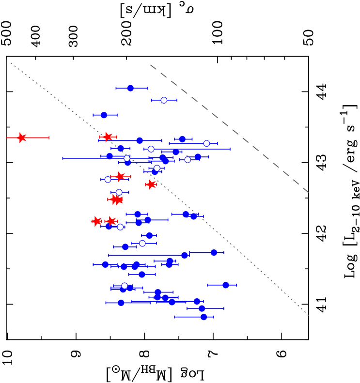
Figure 2: Black hole masses and hard X-ray luminosities of the ‘spectroscopic’ sample of AGN in the CDF-S. Blue open circles: black hole masses estimated using the stellar mass method; red stars: black hole masses calculated from measured host velocity dispersions for the AGN in van der Wel et al. (2005). Solid squares mark objects which show presence of broad lines in optical spectra. Lines (dotted and dashed) denote lines of constant Eddington ratio of 0.01 and 1.0, respectively. Redshift evolution in the $M_{\mathrm{BH}}-\sigma$ relation (e.g. Woo et al. 2006), would cause a shift in all points to higher mass by $\Delta\log M_{\mathrm{BH}}\sim 0.57$.

Also shown on Fig. 2 are black hole masses estimated directly from the van der Wel et al. (2005) velocity dispersion measurements, assuming the zero-redshift relation (3), for the 8 AGN with such measurements. It can be seen that these yield a similar distribution to the stellar mass estimates, as expected from the previous section. This provides independent evidence that systematic contamination from AGN light in the photometric mass estimation is not a significant cause of bias.

Finally, we combine our bolometric luminosities and black hole masses into Eddington ratio estimates. Fig. 3 (shaded histograms) shows the distribution of Eddington ratios for our sample, using both stellar mass and K-magnitude methods. Median (mean) values for the two methods are $\log\lambda=-2.76$ (-2.87) and $-2.64$ (-2.58), respectively.

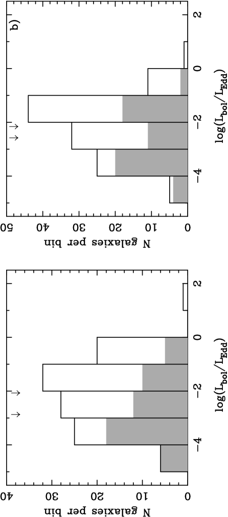
Figure 3: Distribution of Eddington ratios for the ‘spectroscopic’ sample (shaded histogram) using (a) the stellar mass method, (b) the K-magnitude method. Median Eddington ratios are $\log\lambda=-2.87$ and $-2.58$, respectively and the corresponding values are marked with arrows. The solid line histogram shows the distribution of Eddington ratios for the combined ‘spectroscopic’ and ‘photometric’ sample. Median Eddington ratios for the combined distributions are $\log\lambda=-2.07$ and $-2.16$ (marked with arrows). Given the additional uncertainties in the ‘photometric’ sample, the joint sample is expected to be broader than the distribution for the ‘spectroscopic’ sample only. The conclusions are largely unaffected by the choice of sample.

4.2 Analysis of the ‘photometric’ sample

Initially we have a hard X-ray selected sample, but the reduction to the secure redshift and optical–X-ray identification subsample could potentially be biasing us to brighter, and thus likely more massive objects (as they are more likely to have spectroscopic redshift measurement). To test for possible biases of our ‘spectroscopic’ subsample, we use the photometric redshift estimates in CDF-S (Zheng et al. 2004), which are available for $\sim 99\%$ of the X-ray detected sources, with the average redshift accuracy $\sim 8\%$. We supplement the non-secure sample with a combination of photometric catalogues in the field, resulting in photometric data for $\sim 83\%$ of the whole $z<1$ X-ray selected sample. The combined sample colours are less precise than those from the uniform GOODS-MUSIC catalogue. In addition, neither optical identifications nor the photometric redshifts are certain for all objects, so there are likely to be several objects with erroneous Eddington ratio estimates. This makes the catalogue less reliable compared to the ‘spectroscopic’ one, but still the best estimate we can make for the objects missing in our ‘spectroscopic’ sample. We proceed to find stellar mass estimates for the objects. Fits with a well-defined minimum in $\chi^{2}$ are found for 61 out of 66 objects. For broad-line AGN (18 and 11 objects in ‘photometric’ and ‘spectroscopic’ samples, respectively) stellar masses are more likely to be incorrect as the photometry could have a significant contribution from the central object, but we do not remove them from the sample.

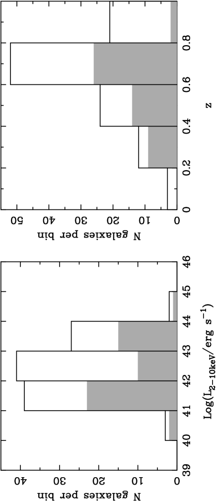
Figure 4: Distributions of absorption-corrected hard X-ray luminosities (left panel) and redshifts (right panel) for the ‘spectroscopic’ sample (shaded histogram) and for the combined ‘spectroscopic’ and ‘photometric’ sample (open histogram). There is a shift to lower X-ray luminosities and to higher redshifts for the ‘photometric’ sample.

We find that the distribution of Eddington ratios for all objects (solid line histogram in Fig. 3), which includes the ‘spectroscopic’ sample (shaded histogram in Fig. 3) and the ‘photometric’ sample, follows closely the distribution of the ‘spectroscopic’ sample, convincing us that our subsample is not biased towards optically bright objects with high black hole masses and low Eddington ratios. Fig. 4 compares the luminosity and redshift distributions of the ‘spectroscopic’ and ‘photometric’ samples. Slightly higher redshifts (mean $\Delta z\sim 0.1$) make the ‘photometric’ sample fainter than the optical spectroscopy limits but those galaxies are not systematically less massive.

5 Discussion

5.1 Distributions of Eddington ratio

The analysis presented here indicates that X-ray selected AGN at the ‘cosmic downsizing epoch’ in fact show a wide range in Eddington ratio, with a median value $\log\lambda\sim-2.8$. We now discuss how this result compares with other determinations of the distribution of AGN Eddington ratios in the literature.

At low redshift, Panessa et al. (2006) find a similarly broad range of Eddington ratio for local Seyfert galaxies selected on the basis of optical spectra. They measured nuclear X-ray fluxes for the galaxies, and find an active nucleus in all but 4 out of 47 Seyfert galaxies. The sample covers the bolometric luminosity range $L_{\mathrm{bol}}\sim 10^{41}-10^{44}$erg s^-1, very similar to the one for our sample, but extending to lower luminosities because of the ability to resolve the nucleus in X-rays. The black hole mass range (estimated mostly from the $M_{\mathrm{BH}}-\sigma$ relation) is almost identical to our sample at $z\sim 0.7$. The estimated Eddington ratios for this sample again have a broad distribution, in the range $\log\lambda=-1$ to $-7$, and median at $\lambda\sim 0.01$ (type 1 AGN) or $\sim 10^{-3}$ (all AGN).

However, for bright ($L_{\mathrm{bol}}\sim 10^{44}-10^{47}$erg s^-1) local AGN, Woo & Urry (2002) find Eddington ratios typically in a narrower range 0.001–0.1, while at $z\sim 0.7$ the ratios are somewhat higher, 0.01–1. For optically selected AGN at $0.3<z<4$, with bolometric luminosities in the range $L_{\mathrm{bol}}\sim 10^{45}-10^{47}$erg s^-1, the Eddington ratios have a narrower distribution (0.1–1), and no apparent redshift dependence (Kollmeier et al. 2006). The most obvious difference with these samples is the different bolometric luminosity range, even at $z<1$.

The variety of reports on Eddington ratio mean value and width of distribution can be understood from the following simple illustration of selection effects. Fig. 5 shows the distribution of Eddington ratio we would expect to observe for samples selected at three differing luminosities. In this illustration, the black hole mass function has been taken to be the double power-law form for ‘active’ black holes of Greene & Ho (2007), the intrinsic distribution of Eddington ratios is taken to be uniform in $\log\lambda$ over the range $-5<\log\lambda<0$, and expected distributions for three choices of bolometric luminosity are shown: $L=0.001L^{\star}$, $0.01L^{\star}$, $0.1L^{\star}$, where $L^{\star}$ is the Eddington luminosity for black holes at the ‘break’ in the double power-law mass function (Greene & Ho 2007 give the black hole mass at the ‘break’ as $M_{\mathrm{BH}}^{\star}=10^{7.32}$ M_⊙ at $z=0$).

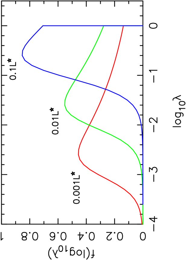
Figure 5: Expected distributions of Eddington ratio $\lambda$ in the simple illustrative model described in the text. Three ‘samples’ are assumed drawn from the active black hole mass function of Greene & Ho (2007), with a uniform intrinsic distribution of $\log(\lambda)$, at luminosities $L=0.001L^{\star}$ (red curve), $0.01L^{\star}$ (green) and $0.1L^{\star}$ (blue).

The illustration demonstrates that, while drawn from the same (unremarkable) intrinsic distribution, the observed Eddington ratio distribution is expected to be strongly dependent on the luminosities probed by an AGN sample: selecting low luminosity objects results in a wide Eddington ratio distribution with a low mean value, whereas selecting high luminosity objects results in a narrow distribution with a high mean Eddington ratio.

Additionally, the observed distribution of $\log\lambda$ is a function not only of the form of the intrinsic distribution but also of the shape of the black hole mass function and the luminosity selection and range covered by the sample. Further selection effects may also arise, if there are systematic variations in AGN SEDs as a function of $\lambda$, as indicated by Boroson (2002) and implied by the difference in Eddington ratios typically seen for type 1 versus type 2 AGN (e.g. Panessa et al. 2006).

5.2 Cosmic downsizing

Similar considerations to those above lead us to conclude that it is necessary to understand the distribution of black hole masses in AGN samples before physical interpretations may be made of the phenomenon of ‘cosmic downsizing’. The most striking result from the analysis presented here is that the AGN responsible for the peak in space density at $z\la 1$ at moderate AGN luminosities cannot be described as being low-mass black holes accreting at high rates. This argues against the simplest interpretation of ‘cosmic downsizing’: the phenomenon is not due to an increasing dominance of low-mass black holes, the typical black hole mass in the CDF-S AGN sample is $\sim 10^{8}$ M_⊙.

Downsizing thus appears to have a rather more complex origin. The typically low Eddington ratios we find could be consistent with the model of Hopkins & Hernquist (2006), where low-level AGN activity is fuelled by stochastic accretion of cold gas, and dominates the AGN population from $z=0$ up to redshifts $z\sim 1$, and at higher redshifts merger-driven AGN fuelling might be dominant. This could be a generic expectation of hierarchical structure formation: merger-driven bright phases of AGN activity exist in high redshift universe, possibly alongside the less bright activity powered by stochastic accretion. At low redshifts, once the mergers become less frequent, stochastic accretion becomes the dominant mode.

More generally, however, if black hole growth is coeval with galaxy growth, then we expect the mean accretion rate onto galaxies, and hence their associated black holes, to decrease with cosmic time (Miller et al. 2006). Indeed, decrease in mean accretion rate must occur, since the integrated AGN luminosity density decreases with cosmic time at $z\la 2$, yet we do not expect the integrated mass in black holes to decrease substantially with time (rather, the latter should increase as black holes continue to grow). Our results suggest that the AGN cosmic downsizing at $z\la 1$ is not a symptom of ‘anti-hierarchical’ behaviour, but in fact may be a reflection of the process of the dying-down of cosmic accretion and a shift in the typical luminosity of massive black holes to lower values. Whether this trend continues to still lower redshift is still an open question: the Panessa et al. (2006) black hole mass and Eddington ratio distribution appear similar to the CDF-S AGN of comparable luminosity, yet it seems that lower-luminosity type 2 AGN at low redshift are dominated by lower mass black holes with moderate Eddington ratios (Heckman et al. 2004).

Finally, we note that for a sample of high-redshift (median $z=2.2$) sub-mm–selected galaxies in the Chandra Deep Field North, Borys et al. (2005) have found that, if their black holes are assumed to be radiating at the Eddington limit, the black hole masses in those high-redshift star-forming galaxies are 1-2 orders of magnitude smaller than in galaxies of comparable mass in the local universe. Given the high redshift of the sample, and the discussion of evolution in mean accretion rate above, it may well be that typical Eddington ratios are higher than for our sample. But interestingly, if we assume that the effect they see is actually from the sub-Eddington accretion rates similar to the ones we report here ($\sim 0.01L_{\mathrm{Edd}}$), this would bring the stellar mass–black hole mass relation for high-redshift star-forming galaxies into agreement with the local one. Reliable black hole mass estimates at higher redshifts would be a key advance in understanding this area.

6 Conclusions

We have estimated Eddington ratios for two samples of hard X-ray selected AGN in CDF-S with median redshift $z=0.7$. The primary ‘spectroscopic’ sample has secure redshifts and optical identifications and spans the bolometric luminosity range $L_{\mathrm{bol}}\sim 10^{41}-10^{45}$erg s^-1. The majority of the sources are radiating at low Eddington ratios in the range $\lambda\sim 1-10^{-5}$, with the median $\log\lambda=-2.87$. A larger sample, based on photometric redshifts, has fewer selection effects, but larger uncertainties related to optical identification and Eddington ratio estimates: this fainter sample has Eddington ratios that span the same range, and the median for the whole sample is $\log\lambda=-2.07$. Black hole masses are in the range $10^{5}-10^{9}\,M_{\odot}$, with the distribution peaking at $\sim 10^{8}\,M_{\odot}$. It is likely that fainter X-ray flux limits would reveal even more sources radiating at low Eddington ratios.

We have discussed how the broad distribution of Eddington ratios arises because of the relatively low luminosities probed by the sample, and that in general observed distributions are strongly dependent on the selected luminosity range of AGN samples. Based on the estimated Eddington ratios and black hole masses for the CDF-S AGN, we argue that diminishing accretion rates onto average-mass supermassive black holes (Miller et al. 2006) are the underlying cause of the observed cosmic AGN downsizing at $z\sim 0.7$, contrary to an interpretation in which most of the activity occurs in rapidly-growing low-mass black holes.