Transformation of auto-Bäcklund type for hyperbolic generalization of Burgers equation

Abstract

We consider the hyperbolic generalization of Burgers equation with polynomial source term. The transformation of auto-Bäcklund type was found. Application of the results is shown in the examples, where the pair of two stationary solutions produces kink and bi-kink solutions.

1 Introduction

In recent years efforts of many scientists were concentrated on the obtaining exact solutions for non-integrable PDE’s. Special attention was paid to solutions describing so-called wave patterns. A number of interesting results was obtained for hyperbolic generalization of Burgers equation (GBE):

$$\tau u_{tt}-\kappa u_{xx}+A\,uu_{x}+B\,u_{t}=f(u)=\lambda(u-m_{1})(u-m_{2})(u-m_{3}).$$ (1)

In the papers [7, 8] equation (1) is derived as a model equation for a generalized Navier-Stokes system taking into account the influence of memory (relaxation) effects. Thanks to the constants $A,\,\,B,\,\,\tau,\,\,\kappa$ GBE can describe a great amount of special cases e.g. for $A=0$ equation (1) coincides with the nonlinear telegraph equation, for $A=B=0$ - with d’Alembert equation, for $\tau=0$ - with Burgers equation etc..

As a nonlinear dissipative equation with outer sources (1) can describe dissipative structures, e.g. soliton- and kink-like solutions. We succeeded in finding out a number of exact and approximated solutions with the help of combining different known methods like Hirota’s ansatz [6], conditional symmetries [3, 9] and qualitative analysis [5]. The number of already known exact solutions to GBE is sufficiently large [10, 11, 12] to pose the problem of their internal structure and interaction. As it is well known the superposition rule cannot be applied in nonlinear case. However for classical Burgers equation

$$\kappa u_{xx}-uu_{x}-u_{t}=0$$ (2)

there exists the auto-Bäcklund transformation

$$u(x,t)=\frac{M(x,t)Exp(h(x,t))+Q(x,t)}{Exp(h(x,t))+1}$$ (3)

stating the nonlinear analog to superposition principle. In fact, for every pair of solutions $M(x,t)$, $Q(x,t)$ there exists a function $h(x,t)$ such that $u(x,t)$ given by (3) is also a solution. The transformation (3) is strongly connected with the Cole-Hopf ansatz. V. G. Danilov, V. P. Maslov and K. A. Volosov [1, 13] used this ansatz considering FitzHygh-Nagumo-Semenov equation:

$$u_{t}-\kappa u_{xx}/(2\,a^{3})=\kappa(u-u^{3}),$$ (4)

which is a particular case of (1). For this equation there was shown, that the set of exact solutions of some special form possesses the structure of a semigroup.
In this paper we make a step forward by stating the conditions of the existence of auto-Bäcklund transformation and certain kind of algebraic structure for some special sets of solutions to GBE.

2 Auto-Bäcklund transformation for GBE

Let us apply the ansatz (3) to GBE. Collecting the coefficients at different powers of $Exp(h(x,t))$ and equating these terms to zero we obtain four equations: $e_{i},\,\,i=0,..,3$:

$$e_{0}:\tau M_{t\,t}(x,t)-\kappa M_{x\,x}(x,t)+A\,M(x,t)M_{x}(x,t)+B\,M_{t}(x,t)-$$ (5)

$$-\lambda(M(x,t)-m_{1})(M(x,t)-m_{2})(M(x,t)-m_{3})=0$$

$$e_{1}:3\lambda\,\,m_{1}\,m_{2}\,m_{3}+B\,M_{t}(x,t)+2\,\tau\,h_{t}(x,t)\,M_{t}(x,t)+2\,B\,Q_{t}(x,t)-2\,\tau\,h_{t}(x,t)\,Q_{t}(x,t)+$$

$$+\tau\,M_{t\,t}(x,t)+2\,\tau\,Q_{t\,t}(x,t)+{Q^{2}(x,t)}\left(\lambda\,(m_{1}+m_{2}+m_{3})-A\,h_{x}(x,t)\right)-$$

$$-2\,\kappa\,h_{x}(x,t)\,M_{x}(x,t)+2\,\kappa\,h_{x}(x,t)\,Q_{x}(x,t)-$$

$$-Q(x,t)\,(2\lambda\,(\,m_{1}\,m_{2}+\,m_{1}\,m_{3}+\,m_{2}\,m_{3})+B\,h_{t}(x,t)+\tau\,{h_{t}^{2}(x,t)}+\tau\,h_{t\,t}(x,t)-$$

$$-\kappa\,{h_{x}^{2}(x,t)}-A\,M_{x}(x,t)-A\,Q_{x}(x,t)-\kappa\,h_{x\,x}(x,t))+M(x,t)\,(-\lambda\,(m_{1}\,m_{2}+m_{1}\,m_{3}+m_{2}\,m_{3})-$$

$$-3\,\lambda\,Q(x,t)^{2}+B\,h_{t}(x,t)+\tau\,{h_{t}(x,t)}^{2}+\tau\,h_{t\,t}(x,t)-\kappa\,{h_{x}^{2}(x,t)}+$$

$$+Q(x,t)\,(2\lambda\,(m_{1}+m_{2}+m_{3})+A\,h_{x}(x,t))+A\,Q_{x}(x,t)-$$

$$-\kappa\,h_{x\,x}(x,t))-\kappa\,M_{x\,x}(x,t)-2\,\kappa\,Q_{x\,x}(x,t)=0$$

$$e_{2}:3\lambda\,m_{1}\,m_{2}\,m_{3}+2\,B\,M_{t}(x,t)+2\,\tau\,h_{t}(x,t)\,M_{t}(x,t)+B\,Q_{t}(x,t)-$$

$$-2\,\tau\,h_{t}(x,t)\,Q_{t}(x,t)+2\,\tau\,M_{t\,t}(x,t)+\tau\,Q_{t\,t}(x,t)+{M^{2}(x,t)}\,(\lambda(m_{1}+m_{2}+m_{3}-3\,Q(x,t))+$$

$$+A\,h_{x}(x,t))-2\,\kappa\,h_{x}(x,t)\,M_{x}(x,t)+2\,\kappa\,h_{x}(x,t)\,Q_{x}(x,t)-$$

$$-Q(x,t)\,(\lambda(m_{1}\,m_{2}+(m_{1}+m_{2})\,m_{3})+h_{t}(x,t)\,(B-\tau\,h_{t}(x,t))+\tau\,h_{t\,t}(x,t)+$$

$$+\kappa\,h^{2}_{x}(x,t)-A\,M_{x}(x,t)-\kappa\,h_{x\,x}(x,t))+M(x,t)\,(-2\lambda\,(m_{1}\,m_{2}+m_{1}\,m_{3}+m_{2}\,m_{3})+$$

$$+h_{t}(x,t)\,(B-\tau\,h_{t}(x,t))+\tau\,h_{t\,t}(x,t)+Q(x,t)\,(2\lambda\,(m_{1}+m_{2}+m_{3})-$$

$$-A\,h_{x}(x,t))+h_{x}(x,t)\,(\kappa\,h_{x}(x,t))+A\,(M_{x}(x,t)+Q_{x}(x,t))-\kappa\,h_{x\,x}(x,t))-$$

$$-2\,\kappa\,M_{x\,x}(x,t)-\kappa\,Q_{x\,x}(x,t)=0$$

$$e_{3}:\tau Q_{t\,t}(x,t)-\kappa Q_{x\,x}(x,t)+AQ(x,t)Q_{x}(x,t)+BQ_{t}(x,t)-$$

$$-\lambda(Q(x,t)-m_{1})(Q(x,t)-m_{2})(Q(x,t)-m_{3})=0.$$

The key fact for our further considerations is that two of them, namely $e_{0}$ and $e_{3}$ are GBE (1) written for $M(x,t)$ and $Q(x,t)$. The equations $e_{1}$ and $e_{2}$ seem to have quite complicated form. To simplify these equations, we calculate $M_{x\,x}(x,t)$ and $Q_{x\,x}(x,t)$ from $e_{0}$ and $e_{3}$, put them into $(e_{1},\,\,e_{2})$ and consider the system $(e_{2}-e_{1},\,\,e_{1})$. Additionally we introduce the new auxiliary function $P(x,t)=M(x,t)-Q(x,t)$. Finally the system (5) takes the form $(e_{0},\,e_{3},\,e_{4},\,e_{5})$, where

$$e_{4}={P^{2}(x,t)}-2\,\tau\,{h_{t}^{2}(x,t)}+A\,P(x,t)\,h_{x}(x,t)+2\,\kappa\,{h_{x}^{2}(x,t)}=0,$$ (6)

$$e_{5}={P^{3}(x,t)}-\lambda\,(m_{1}+m_{2}+m_{3})\,P^{2}(x,t)+3\,{P^{2}(x,t)}\,Q(x,t)+2\,\tau\,h_{t}(x,t)\,P_{t}(x,t)-$$ (7)

$$-2\,\kappa\,h_{x}(x,t)\,P_{x}(x,t)+P(x,t)\,(B\,h_{t}(x,t)+\tau\,{h_{t}^{2}(x,t)}+\tau\,h_{t\,t}(x,t)+$$

$$+A\,Q(x,t)\,h_{x}(x,t)-\kappa\,{h_{x}^{2}(x,t)}-A\,P_{x}(x,t)-\kappa\,h_{x\,x}(x,t))=0.$$

Let us note that using the standard scaling transformation $t=e^{\alpha}\,\hat{t},\,\,x=e^{\beta}\,\hat{x},\,\,u=e^{\gamma}\,\hat{u}$ one can manipulate some of the parameters. So in further considerations without loss of the generality we shall assume that $\kappa=1$ while $A=2\sqrt{2}$. In this case (1) takes form:

$$\tau\,u_{tt}+2\sqrt{2}\,uu_{x}+B\,u_{t}-u_{xx}=\lambda(u-m_{1})(u-m_{2})(u-m_{3})$$ (8)

and $e_{4}$ becomes linear:

$$e_{4}=\pm\sqrt{2\,\tau}\,{h_{t}(x,t)}-P(x,t)-\sqrt{2}\,{h_{x}(x,t)}=0.$$ (9)

Further on we take into account only ”+”, since the results for the other possibility are symmetric. Solution of (9) can be found in [4]:

$$h(x,t)=\frac{1}{\sqrt{2\,\tau}}\int_{0}^{x}P(\xi-\frac{t}{\sqrt{\tau}},\,t)d\xi+\Phi(x+\frac{t}{\sqrt{\tau}}),$$ (10)

where $\Phi$ is some arbitrary smooth function.

We can formulate the results in the form of following lemma:

Lemma 1

If the functions $M(x,t),\,\,Q(x,t)$ satisfy GBE (1), $h(x,t)$ is given by (10) and the compatibility condition (7) is fulfilled, then

$$u(x,t)=\frac{M(x,t)Exp(h(x,t))+Q(x,t)}{Exp(h(x,t))+1}$$

is the solution to GBE (1).

The above lemma shows, that when the equations (7,10) are satisfied the pair of solutions to GBE (1) can produce a new one. Our aim is to define a set of solutions, which pairwise correspond to a certain function $h(x,t)$ and satisfy the compatibility condition (7). Further steps will be as follows: first we introduce certain equivalence relation between the solutions. Then we consider equivalence class of the constant solution $u(x,t)=m_{1}$ and inside this class we build a semi-algebraic structure. The examples of applications are given in the last section.

3 Equivalence relation

Definition 1

Let $M(x,t)=\frac{M_{1}(x,t)Exp(h_{1}(x,t))+Q_{1}(x,t)}{Exp(h_{1}(x,t))+1}$,
$Q(x,t)=\frac{M_{2}(x,t)Exp(h_{2}(x,t))+Q_{2}(x,t)}{Exp(h_{2}(x,t))+1}$ be the pair of solutions to (8). $M(x,t)$ and $Q(x,t)$ are said to be in relation ( $M(x,t)\sim Q(x,t)$) if and only if there exists a function $h(x,t)$ of the form (10) such that $M(x,t),\,\,Q(x,t)$ and $h(x,t)$ satisfy (7).

Theorem 1

The relation stated by definition (1) is an equivalence relation if $B$ is of the form:

$$B=-\frac{4\,\lambda\,({m_{1}}+{m_{2}}+{m_{3}})\,\sqrt{\tau}}{\sqrt{2}}.$$ (11)

Proof:

1. Reflexivity: $M(x,t)\sim M(x,t)$
$u(x,t)=\frac{M(x,t)Exp(h(x,t))+M(x,t)}{Exp(h(x,t))+1}=M(x,t)$ is a GBE solution for $h(x,t)=0$.

2. Symmetry: $M(x,t)\sim Q(x,t)\Leftrightarrow Q(x,t)\sim M(x,t)$

We assume, that the conditions (7, 10) are satisfied for $P(x,t)=M(x,t)-Q(x,t)$ and $h(x,t)$. Let us find $\tilde{h}(x,t)$ for $\tilde{P}(x,t)=Q(x,t)-M(x,t)=-P(x,t)$.
The condition (10) for ($P(x,t),\,\,h(x,t)$) is

$$\sqrt{2\,\tau}\,{h_{t}(x,t)}-P(x,t)-\sqrt{2}\,{h_{x}(x,t)}=0.$$

For ($-P(x,t),\,\,\tilde{h}(x,t)$):

$$\sqrt{2\,\tau}\,{\tilde{h}_{t}(x,t)}+P(x,t)-\sqrt{2}\,{\tilde{h}_{x}(x,t)}=0.$$

It is easy to see, that $\tilde{h}(x,t)=-h(x,t)$ is a right choice. Now we check the second condition (7) for the pair ($-P(x,t),\,\,-h(x,t)$):

$$-{P(x,t)}^{3}-\lambda\,(m_{1}+m_{2}+m_{3})\,P^{2}(x,t)+3\,{P(x,t)}^{2}\,M(x,t)+2\,\tau\,h_{t}(x,t)\,P_{t}(x,t)$$ (12)

$$-2\,h_{x}(x,t)\,P_{x}(x,t)-P(x,t)\,(-B\,h_{t}(x,t)+\tau\,{h_{t}(x,t)}^{2}-\tau\,h_{t\,t}(x,t)-$$

$$-2\sqrt{2}\,M(x,t)\,h_{x}(x,t)-\,{h_{x}(x,t)}^{2}+2\sqrt{2\,}\,P_{x}(x,t)+\,h_{x\,x}(x,t))=0.$$

Adding (7) and (12) results in:

$${P(x,t)}^{2}-2\,\tau\,{h_{t}(x,t)}^{2}+2\sqrt{2}\,P(x,t)\,h_{x}(x,t)+2\,{h_{x}(x,t)}^{2}=0,$$

which is satisfied by assumptions.

3. Transitivity: $M_{1}(x,t)\sim Q_{1}(x,t),\,\,Q_{1}(x,t)\sim M_{2}(x,t)\Rightarrow M_{1}(x,t)\sim M_{2}(x,t)$
We assume, that ($M_{1}(x,t),\,\,Q_{1}(x,t)$) and ($Q_{1}(x,t),\,\,M_{2}(x,t))$ satisfy (7, 10) with respectively $h_{1}(x,t),\,\,h_{2}(x,t)$. From (10) we can calculate:

$$P_{1}(x,t)=M_{1}(x,t)-Q_{1}(x,t)=\sqrt{2\,\tau}\,{h_{1\,t}(x,t)}-\sqrt{2}\,{h_{1\,x}(x,t)}$$

$$P_{2}(x,t)=Q_{1}(x,t)-M_{2}(x,t)=\sqrt{2\,\tau}\,h_{2\,t}(x,t)-\sqrt{2}\,h_{2\,x}(x,t).$$

Since we want $M_{1}(x,t)$ to be in the relation with $M_{2}(x,t)$ then we need some $h(x,t)$, which satisfies:

$$P(x,t)=M_{1}(x,t)-M_{2}(x,t)=\sqrt{2\,\tau}\,h_{t}(x,t)-\sqrt{2}\,h_{x}(x,t).$$

$P(x,t)$ can be written in terms of $h_{1}(x,t),\,\,h_{2}(x,t)$:

$$P(x,t)=P_{1}(x,t)+P_{2}(x,t)=\sqrt{2\,\tau}(h_{1\,t}(x,t)+h_{2\,t}(x,t))-\sqrt{2}\,(h_{1\,x}(x,t)+h_{2\,x}(x,t))$$

and we can put

$$h(x,t)=h_{1}(x,t)+h_{2}(x,t).$$

In order to check (7) for $h(x,t)$ we use the following procedure: in the first step we eliminate $h_{1\,x\,x}(x,t)$ and $h_{2\,x\,x}(x,t)$ from the corresponding versions of (7), next we use them in (7) for $h(x,t)$, with additional facts that $M_{1}(x,t)=P_{1}(x,t)+Q_{1}(x,t)$, $M_{2}(x,t)=P_{2}(x,t)+Q_{1}(x,t)$. Simple but quite cumbersome calculations provide us the additional condition (11).

 

Notation 1

$\Gamma$ denotes the equivalence class of the stationary solution $u(x,t)=m_{1}$ to (8). ($\Gamma=[m_{1}]_{\sim}$).

Construction of the set $\Gamma$ implies, that the elements of $\Gamma$ pairwise can produce another solutions. In the next part we introduce some algebraic structure within this set. This structure is very important for estimation of number of truly new solutions. Let us also note, that $\Gamma$ is not empty since at least it contains the stationary solution $m_{1}$.

4 Algebraic-like structure

Definition 2

For a given $h(x,t)$ satisfying (10) we define operation in $\Gamma$:

$$M(x,t)\circ_{h}Q(x,t)=\frac{M(x,t)Exp\,(h(x,t))+Q(x,t)}{Exp\,(h(x,t))+1}.$$

Lemma 2

$\Gamma$ is closed with respect to the operation ”$\circ_{h}$”. In other words $M(x,t),\,Q(x,t)\in\Gamma\Rightarrow\exists h(x,t):$ $M(x,t)\circ_{h}Q(x,t)\in\Gamma.$

Proof:
Since $M(x,t)\in[m_{1}]_{\sim}$ and $Q(x,t)\in[m_{1}]_{\sim}$ the transitivity of relation $\sim$ provides $M(x,t)\sim Q(x,t)$. So there exists function $h_{1}(x,t)$ such that $u(x,t)=M(x,t)\circ_{h_{1}}Q(x,t)$ is a solution of (8). We have to check, whether $u(x,t)\in[m_{1}]_{\sim}$. In order to do that we have to find $h(x,t)$ such that $u(x,t)\circ_{h}m_{1}$ is also a solution of (8).
Let the pair $(M(x,t),m_{1})$ correspond to the function $h_{2}(x,t)$, then from the equation (9) written for that pair we obtain:

$$M(x,t)=\sqrt{2\,\tau}\,h_{2\,t}(x,t)-\sqrt{2}\,h_{2\,x}(x,t)+m_{1}.$$

The same equation (9) written for the pair $(M(x,t),Q(x,t))$:

$$M(x,t)-Q(x,t)=\sqrt{2\,\tau}\,h_{1\,t}(x,t)-\sqrt{2}\,h_{1\,x}(x,t)\Rightarrow$$

$$\,\,\,\,\,\,\,\,\,\,\,\,\,\,\Rightarrow Q(x,t)=\sqrt{2\,\tau}\,(h_{2\,t}(x,t)-h_{1\,t}(x,t))-\sqrt{2}\,(h_{2\,x}(x,t)-h_{1\,x}(x,t))-m_{1}.$$

Hence the function $h(x,t)$ must satisfy:

$$\sqrt{2\,\tau}\,h_{\,t}(x,t)-\sqrt{2}\,h_{\,x}(x,t)=M(x,t)\circ_{h_{1}}Q(x,t)-m_{1}=$$

$$=\frac{M(x,t)Exp(h_{1}(x,t))+Q(x,t)}{Exp(h_{1}(x,t))+1}-m_{1}=\frac{(\sqrt{2\,\tau}\,h_{2\,t}(x,t)-\sqrt{2}\,h_{2\,x}(x,t)+m_{1})Exp(h_{1}(x,t))}{Exp(h_{1}(x,t))+1}+$$

$$+\frac{\sqrt{2\,\tau}\,(h_{2\,t}(x,t)-h_{1\,t}(x,t))-\sqrt{2}\,(h_{2\,x}(x,t)-h_{1\,x}(x,t))-m_{1}}{Exp(h_{1}(x,t))+1}-m_{1}=$$

$$=\sqrt{2\tau}\left(h_{2\,t}(x,t)-\frac{h_{1\,t}(x,t)}{Exp(h_{1}(x,t))+1}\right)-\sqrt{2}\left(h_{2\,x}(x,t)-\frac{h_{1\,x}(x,t)}{Exp(h_{1}(x,t))+1}\right).$$

If we put

$$h(x,t)=h_{2}(x,t)-h_{1}(x,t)+Ln(1+Exp(h_{1}(x,t))),$$ (13)

then condition (7) can be easily checked by direct substitution.

 

Theorem 2

$\Gamma$ has the following properties:
a) Any element of $\Gamma$ is the unity for itself: $M(x,t)\circ_{0}M(x,t)=M(x,t)$
b) The operation is commutative: $M(x,t)\circ_{h}Q(x,t)=Q(x,t)\circ_{-h}M(x,t)$
c) Association property: $M_{1}(x,t)\circ_{H_{1}}(Q_{1}(x,t)\circ_{-h_{2}}M_{2}(x,t))=(M_{1}(x,t)\circ_{h_{1}}Q_{1}(x,t))\circ_{H_{2}}M_{2}(x,t)$, where $H_{1}(x,t)=-Ln\frac{1+Exp(-h_{2}(x,t))}{Exp(h_{1}(x,t))}$ and $H_{2}(x,t)=Ln\frac{1+Exp(h_{1}(x,t))}{Exp(h_{2}(x,t))}$.

Proof:
a) The pair $(M(x,t),M(x,t))$ may correspond to the function $h(x,t)=0$, so:

$$M(x,t)\circ_{0}M(x,t)=\frac{M(x,t)Exp(0)+M(x,t)}{Exp(0)+1}=M(x,t)$$

b) From the theorem 1 we know, that if the pair $(M(x,t),Q(x,t))$ corresponds to $h(x,t)$ then $(Q(x,t),M(x,t))$ is connected with $-h(x,t)$.

$$M(x,t)\circ_{h}Q(x,t)=\frac{M(x,t)Exp(h(x,t))+Q(x,t)}{Exp(h(x,t))+1}=$$

$$=\frac{Q(x,t)Exp(-h(x,t))+M(x,t)}{Exp(-h(x,t))+1}=Q(x,t)\circ_{-h}M(x,t)$$

c) We assume that the pairs $(M_{1}(x,t),Q_{1}(x,t))$ and $(M_{2}(x,t),Q_{1}(x,t))$ are connected respectively with $h_{1}(x,t)$ and $h_{2}(x,t)$. To find $H_{2}(x,t)$ we write down (9) for the pairs $(M_{1}(x,t),Q_{1}(x,t))$, $(M_{2}(x,t),Q_{1}(x,t)),$ $(M_{1}(x,t)\circ(Q_{1}(x,t)),M_{2}(x,t))$ and next execute the calculations similar to lemma 2. Finally we obtain:

$$H_{2}(x,t)=\int\frac{Exp(h_{1}(x,t))}{Exp(h_{1}(x,t))+1}h_{1\,x}(x,t)-h_{2\,x}(x,t)dx=Ln\frac{1+Exp(h_{1}(x,t))}{Exp(h_{2}(x,t))}.$$

Since the pair $(M_{1}(x,t)\circ\,Q_{1}(x,t)),M_{2}(x,t))$ corresponds to $H_{2}(x,t)=Ln\frac{1+Exp(h_{1}(x,t))}{Exp(h_{2}(x,t))}$, the proper function for $(M_{1}(x,t)\circ\,Q_{1}(x,t),M_{2}(x,t))$ would be $H_{1}(x,t)=-Ln\frac{1+Exp(-h_{2}(x,t))}{Exp(h_{1}(x,t))}$. Direct substitution finishes the proof.

 

Let us note, that the results of present section implies that $(M(x,t)\circ\,Q(x,t))\circ\,Q(x,t)=M(x,t)\circ(Q(x,t)\circ Q(x,t))=M(x,t)\circ Q(x,t)$. It means, that the finite set of the solutions can produce only finite number of new ones.

5 Examples

Let $Q(x,t)=m_{1}$, $M(x,t)=m_{2}$, $\lambda=1$. It is easy to check, that $M(x,t),\,Q(x,t)\in\Gamma$. Then for $P(x,t)=M(x,t)-Q(x,t)=m_{2}-m_{1}$ the equation (9) can be written as follows:

$${\sqrt{2\,\tau}}\,h_{\,t}(x,t)-{\sqrt{2}}\,h_{\,x}(x,t)+m_{1}-m_{2}=0,$$

so the function $h(x,t)$ can be easily calculated:

$$h(x,t)=\frac{(m_{1}-m_{2})\,x}{{\sqrt{2}}}+\phi(t+x\,\sqrt{\tau}).$$

The compatibility condition (7) takes form:

$$\left(2\,m_{3}+m_{2}+m_{1}\right)(m_{2}-m_{1}+2\,\sqrt{2\,\tau}\,\phi^{\prime}(t+x\,\sqrt{\tau}))=0.$$ (14)

The solutions of the above equation (14) are as follows:

$$\phi(t+x\,\sqrt{\tau})=\frac{(m_{1}-m_{2})\,(t+x\,\sqrt{\tau})}{2\,\sqrt{2\,\tau}}+c$$ (15)

or

$$m_{1}=-m_{2}-2\,m_{3}.$$ (16)

In the first case (15) function $h(x,t)$ is of the form:

$$h(x,t)=\frac{m_{1}-m_{2}}{2\,\sqrt{2\,\tau}}(3\sqrt{\tau}\,x+t)$$

and we obtain a solution of kink type:

$$u(x,t)=\frac{m_{2}\,Exp(\frac{m_{1}-m_{2}}{2\,\sqrt{2\,\tau}}(3\sqrt{\tau}\,x+t))+m_{1}}{Exp(\frac{m_{1}-m_{2}}{2\,\sqrt{2\,\tau}}(3\sqrt{\tau}\,x+t))+1}.$$ (17)

For $m_{1}=\tau=1$, $m_{2}=0$ this solution is presented on the figure 1.

In the second case (16) we can choose smooth function $\phi(t+x\,\sqrt{\tau})$ arbitrary. For example we can take

$$\phi(t+x\,\sqrt{\tau})=Sin(t+x\,\sqrt{\tau}).$$

Then we obtain a solution of the form:

$$u(x,t)=m_{2}-\frac{2(m_{2}+m_{3})}{1+Exp(-\sqrt{2}\,(m_{2}+m_{3})\,x+Sin(t+x\,\sqrt{\tau}))}.$$ (18)

Such a solution corresponds to the periodic kink solution presented on the figure 2 for the parameters $\tau=1,\,\,m_{2}=2,\,\,m_{3}=1$.

For

$$\phi(t+x\,\sqrt{\tau})=Log\left(\frac{1+Exp(t+x\,\sqrt{\tau})\,R}{1+Exp(t+x\,\sqrt{\tau})}\right)$$

we obtain a bi-kink solution:

$$u(x,t)=\frac{m_{2}\,Exp(\omega_{1})[1+R\,Exp(\omega_{2})]}{1+Exp(\omega_{1})+Exp(\omega_{2})+R\,Exp(\omega_{1}+\omega_{2})},$$ (19)

where $\omega_{1}=-\frac{m_{2}\,x}{\sqrt{2}},\,\,\,\omega_{2}=t+x\,\sqrt{\tau}.$
For $\tau=1,\,\,m_{3}=-0.1,\,\,R=0.001$ it has the form:

$$u(x,t)=\frac{e^{t}-2\,e^{x}}{e^{t}+e^{\frac{5\,t}{4}+\frac{x}{2}}+2\,e^{x}}$$

and presented on the figure 3.

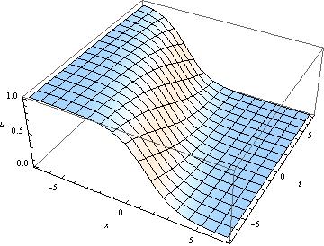
Figure 1: Plot of the solution (17) for $\tau=1,\,\,m_{1}=1,\,\,m_{2}=0$

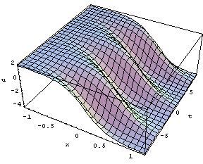
Figure 2: Plot of the solution (18) for $\tau=1,\,\,m_{2}=2,\,\,m_{3}=1$

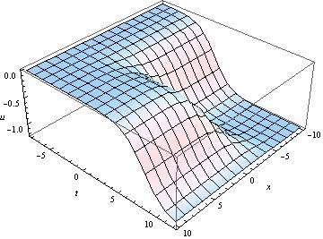
Figure 3: Plot of the solution (19) for $\tau=1,\,\,m_{3}=-0.1,\,\,R=0.001$

6 Conclusions

We considered the hyperbolic generalization of Burgers equation (1) and the ansatz (3), which plays role of auto-Bäcklund transformation for classical Burgers equation. For generalized equation we obtained the formula (10) describing function $h(x,t)$ and the compatibility condition (7). The equivalence class $\Gamma$ was constructed in a way allowing to ”join” every pair of solutions in a new one. Some algebraic properties of this set was stated. The examples in the last section illustrate the possibility of practical application of these results. Two trivial stationary solutions from the set $\Gamma$ were used to obtain a wide class of kink and bi-kink solutions.

References

- [1] V.G. Danilov, V.P. Maslov, K.A. Volosov, Mathematical Modelling of Heat and Mass Transfer Processes, Kluwer Academic Publishers, Dordrecht, Boston, London, 1995.
- [2] R.K. Dodd, J.C. Eilbek, J.D. Gibbon, H.C. Morris, Solitons and Nonlinear Wave Equations, Academic Press, London, 1984.
- [3] V. Fushchich, I. Tsyfra, J. Phys. A: Math. Gen., 20, 1985, L45–L48.
- [4] L.C. Evans, Partial Differential Equations, AMS, 1998.
- [5] J. Guckenheimer, P. Holmes, Nonlinear Oscillations, Dynamical Systems and Bifurcations of Vector Fields, Springer, New York, 1987.
- [6] R. Hirota, J. Phys. Soc. Jpn., 33, 1972, 1459.
- [7] A.S. Makarenko, Control and Cybernetics, 25, 621–630, 1996.
- [8] A.S. Makarenko, M.N. Moskalkov, S.P. Levkov, Phys. Let. A, 235, 1997, 391–397.
- [9] P. Olver, E. Vorob’jev, Nonclassical and conditional symmetries, in: CRC Handbook of Lie Group Analysis of Differential Equations. CRC Press Inc, 2000.
- [10] V.A. Vladimirov, E.V. Kutafina, Rep. Math. Physics, 54, 2004, 261-271.
- [11] E.V. Kutafina, V.A. Vladimirov, Collection of Works of Math. Inst. of Science Akademy of Ukraine, 2006, vol.3, pp. 170-181.
- [12] V.A. Vladimirov, E.V. Kutafina, Rep. Math. Physics, vol. 58/3, 2006.
- [13] K.A. Volosov, Mathematical Notes, vol. 71, no. 3, 2002, pp. 339 354.