A scene model of exosolar systems for use in planetary detection and characterisation simulations

Abstract

Context. Instrumental projects that will improve the direct optical finding and characterisation of exoplanets have advanced sufficiently to trigger organized investigation and development of corresponding signal processing algorithms. The first step is the availability of field-of-view (FOV) models. These can then be submitted to various instrumental models, which in turn produce simulated data, enabling the testing of processing algorithms.

Aims. We aim to set the specifications of a physical model for typical FOVs of these instruments.

Methods. The dynamic in resolution and flux between the various sources present in such a FOV imposes a multiscale, independent layer approach. From review of current literature and through extrapolations from currently available data and models, we derive the features of each source-type in the field of view likely to pass the instrumental filter at exo-Earth level.

Results. Stellar limb darkening is shown to cause bias in leakage calibration if unaccounted for. Occurrence of perturbing background stars or galaxies in the typical FOV is unlikely. We extract galactic interstellar medium background emissions for current target lists. Galactic background can be considered uniform over the FOV, and it should show no significant drift with parallax. Our model specifications have been embedded into a Java simulator, soon to be made open-source. We have also designed an associated FITS input/output format standard that we present here.

1 Introduction

Instruments currently under design for direct optical exoplanetary search and characterisation need to go beyond the indirect techniques used so far for the discovery of the $\sim 200$ currently known exoplanets, and must collect planetary photons. Beyond the joint determination of the science objectives of albedo, planetary radius and orbital parameters, the major aim of these instruments is to establish the presence, in a potential atmosphere, of chemical markers of life processes (biomarkers). This would be done through the detection of their absorption features in the spectral flux emitted by the planet.

Because of this, broadband observation is required. Two types of spaceborne instruments are currently under development. Both types of instruments reject stellar light, so that the 10^-9 and 10^-6 respectively weaker planetary flux is detectable in the residual noise. The Terrestrial Planet Finder Coronograph (TPF-C) is a $6\times 2\leavevmode\nobreak\ \mathrm{m}^{2}$ monolithic collector space telescope in the visible (Traub et al. 2006). Free-flying-collector interferometers, in the infrared (band extending from 6 to 18 $\micro\mathrm{m}$), used in a particular optical design called nulling interferometry (Bracewell 1978), are also being considered. In this latter technique, the optical array is phased so that light from the on-axis star is destructively interfered. As the array is rotated, the off-axis planets pass through the peaks and valleys of the instrumental response on the sky (the so-called transmission map), which generates a modulated signal. The main interferometric projects are Darwin (Leger et al. 1996; Fridlund 2000) and TPF-I (Beichman et al. 1999). Complementarity of biomarkers at these two wavelength ranges, associated with the advantages and shortcomings of each of these classes of instruments, explain this parallel effort.

Both approaches are currently mature enough to trigger organized investigation and development of signal processing algorithms for planet detection and characterisation: Ferrari et al. (2006) for direct imaging, and Mugnier et al. (2006), Thiébaut & Mugnier (2006), Thi baut et al. (2007), Marsh et al. (2006), Draper et al. (2006) for nulling interferometry.

This paper specifies a physical and mathematical model of source FOVs, called Origin. As will be seen in the various sections of this paper, there is an abundance of available elements characterizing exoplanetary FOVs. We felt there was a need for an integrated access to this information for simulation input, data exchange and outreach.

At the present time, the instruments capable of exo-Earth detection and characterisation are in a very early definition phase: no concepts are considered final. For this reason we make no simplifying assumption regarding the instrument, in particular its sensitivity and/or its ability to discriminate between specific scene features and/or noise sources.

This work has been greatly inspired by the European Darwin mission, hence the nulling interferometry point of view is often significantly developed beyond the conclusions that apply more generally to exo-Earth finding instruments.

2 Framework

In this section we present the framework elements of our model: the building-block rationale and considerations on spatial, spectral and temporal resolutions.

2.1 Building-Block Model

Our simulator of astronomical scenes aims at modeling the angular and spectral distribution of light received from the observed exoplanetary system. The proposed model is built by superimposing the emission of the various sources that are seen by the instrument. Following this, the specific intensity (units: $\mathrm{W\,m^{-2}\,rad^{-2}\,\micro\mathrm{m}^{-1}}$) observed in a direction $\mathbf{s}$ is:

$$I(\mathbf{s},\lambda,t) = I_{\star}(\mathbf{s},\lambda,t)+\sum_{j}I_{j}(\mathbf{s},\lambda,t)$$ (1)

$$\mbox{}+I_{\mathrm{ez}}(\mathbf{s},\lambda,t)+I_{\mathrm{z}}(\lambda,t)+I_{\mathrm{bg}}(\mathbf{s},\lambda,t)\,,$$

where $I_{\star}$ is the star’s emission (see Sect. 3), $I_{j}$ is the contribution of the $j$-th planet (see Sect. 4), $I_{\mathrm{ez}}$ is the emission by the exozodiacal cloud (see Sect. 5.2), $I_{\mathrm{z}}$ is the local zodiacal cloud emission assumed to be uniform across the field of view (see Sect. 5.1) and, finally, $I_{\mathrm{bg}}$ accounts for the contribution of background sources (Sect. 5.3 and Sect. 5.4). If $(x,y)$ are the cartesian coordinates of a given source in a plane perpendicular to the line of sight, then the angular direction of observation with respect to the center of the field of view is $\mathbf{s}\simeq{\color[rgb]{0.10,0.60,0.10}(\theta_{\mathrm{x}},\theta_{\mathrm{y}})=}\,(x,y)/d$, where $d$ is the distance from the observer.

For each source type, the various sections of this paper will present a discussion on the astrophysical features likely to pass the instrumental filter, at the level of the signal that an exo-Earth would produce, and hence which require modeling; subsequently, example layer-outputs for that particular source are demonstrated.

2.2 Coordinates Systems

Our model accounts for the observatory’s Solar-system coordinates (ecliptic, Earth or L2) and for target coordinates, enabling local zodiacal drift computing (see Sect. 5.1). The planed vertical extent (under $7\times 10^{5}$ km ) of the observatory’s halo Lissajous libration orbit around L2 (Landgraf 2004) is considered small compared to the zodiacal cloud’s thickness, and was not implemented.

A target (i.e. exosystem)-proper coordinate system is implemented for calculation of the stellar flux received and phase-reflected by a planet (Sect. 4.2). It also enables consistent scene generation for revisits, astrophysical community databases import/export, and robustness testing of image reconstruction algorithms.

Temporal accounting has two aspects. Time is used to model variations in the scene that occur typically on timescales comparable to those of an observation, such as the motion of close, short revolution-period planets (Pegasides), or stellar variability (flares). The resolution is typically 1/10^th of an hour. Dates are used to initialize scene consistently, for simulating revisits; the same 1/10^th hour resolution applies, but expressed in fractional Julian Date (JD). In the output of our model, we assume that the exposure duration $\Delta{}t$ is sufficiently short to consider that the scene is static during a given exposure.

2.3 Spatial Resolution

In the output of the proposed building-block model (see Appendix B), sources with apparent size larger than the instrumental resolution must be considered as resolved, and modeled by maps of their brightness distribution. These maps (or images) must be sampled with a pixel size $\Delta\theta$ smaller than the instrumental resolution limit:

$$\Delta\theta\ll\frac{\lambda_{\mathrm{min}}}{B_{\mathrm{max}}}$$ (2)

where $\lambda_{\mathrm{min}}$ is the smallest spectral channel effective wavelength, and $B_{\mathrm{max}}$ the largest interferometric baseline. For a monolithic telescope, $B_{\mathrm{max}}$ is the diameter of the pupil.

2.4 Spectral Resolution

To avoid loss of coherence in the interferometer model due to the finite spectral bandwidth $\Delta\lambda$ in the scene model, the spectral resolution must be chosen so that the phase difference across a spectral channel is negligible:

$$\left|\frac{B\,\theta}{\lambda-\frac{1}{2}\,\Delta\lambda}-\frac{B\,\theta}{\lambda+\frac{1}{2}\,\Delta\lambda}\right|\simeq\frac{B\,\theta\,\Delta\lambda}{\lambda^{2}}\ll 1$$ (3)

where $\lambda$ is the effective wavelength of the spectral channel, $B$ is the interferometric baseline, and $\theta$ is the view angle. Hence the spectral resolution must be chosen so that:

$$\frac{\lambda}{\Delta\lambda}\gg\frac{B_{\mathrm{max}}\,\theta_{\mathrm{max}}}{\lambda}$$ (4)

where $\theta_{\mathrm{max}}$ is the radius of the field of view.

The interferometric baseline is typically chosen so as to have the dark fringe of the nulling interferometer not larger than the inner size $\theta_{\mathrm{HZ}_{\mathrm{in}}}$ of the habitable zone, that is: $\lambda/B_{\mathrm{max}}\sim\theta_{\mathrm{HZ}_{\mathrm{in}}}$. Assuming a typical field of view radius of $\theta_{\mathrm{max}}\sim 0\aas@@fstack{\prime\prime}5$, and since the smallest considered $\theta_{\mathrm{HZ}_{\mathrm{in}}}$ is $0\aas@@fstack{\prime\prime}01\leavevmode\nobreak\ mas$ (Kaltenegger et al. 2006), the spectral resolution must be better than $\sim 50$.

2.5 Photon Counts

To produce an image, it is convenient to first consider the expression of the photon count received into a spectral channel by a pixel during an exposure. For a resolved source this is:

$$N_{\mathrm{resolved}}=\eta_{\lambda}\,\mathcal{S}_{\mathrm{tel}}\,\frac{\lambda}{h\,c}\,I(\mathbf{s},\lambda,t)\,\Delta\theta^{2}\,\Delta\lambda\,\Delta{}t\,,$$ (5)

where $\Delta{}t$ is the exposure duration, $\mathcal{S}_{\mathrm{tel}}$ is the collecting area (e.g. unobstructed surface of the telescope primary mirror) and $\eta_{\lambda}$ is the instrumental throughput at the spectral channel wavelength. The photon count in Eq. (5) assumes that the spectral bandwidth $\Delta\lambda$, the pixel size $\Delta\theta$, and the exposure $\Delta{}t$ are small enough compared to typical scales of variation of the specific intensity $I(\mathbf{s},\lambda,t)$, as discussed in the previous subsections.

For an unresolved source (e.g. a planet or any point-like source), the term $I(\mathbf{s},\lambda,t)\,\Delta\theta^{2}$ in Eq. (5) must be replaced by the specific flux $F(\lambda,t)$. For the planets, the specific flux can be computed straightforwardly from atmospheric models (Sect. 4.1) which are used as input databases in our building-block model. The number of photons received by a pixel is thus:

$$N_{\mathrm{unresolved}}=\eta_{\lambda}\,\mathcal{S}_{\mathrm{tel}}\,\frac{\lambda}{h\,c}\,F(\lambda,t)\,\Delta\lambda\,\Delta{}t\,.$$ (6)

The building-block output of our model comprises two categories, accordingly. For resolved sources such as the exozodiacal dust emission, the output consists of 3-D $(\theta_{\mathrm{x}},\theta_{\mathrm{y}},\lambda)$ maps of the brightness distribution of the source at a given observing time $t$, and integrated by a pixel of angular size $\Delta\theta$ and effective spectral bandwidth $\Delta\lambda$:

$$f_{\mathrm{resolved}}(\mathbf{s},\lambda,t)=\frac{\lambda\,I(\mathbf{s},\lambda,t)}{h\,c}\,\Delta\theta^{2}\,\Delta\lambda$$ (7)

in units of number of incident photons per $\mathrm{m}^{2}$ per $\mathrm{s}$. For unresolved sources, such as the planets, the building-block model output is simply the specific flux of the point-like source integrated in every spectral channel at a given observing time $t$:

$$f_{\mathrm{unresolved}}(\lambda,t)=\frac{\lambda\,F(\lambda,t)}{h\,c}\,\Delta\lambda$$ (8)

in the same units as $f_{\mathrm{resolved}}$.

3 Star Model

This section describes the modeling of $I_{\star}(\mathbf{s},\lambda,t)$, the specific intensity emitted by the star.

3.1 Limb Darkening and Stellar Leakage

Due to the finite extension of the star, coupled with instrumental instabilities, the stellar light may not be completely suppressed by the coronagraphic technique, be it classical or interferometric coronagraphy. The residual light is called leakage. We would like to know if choosing not to model the stellar limb darkening would lead to significant errors of the leakage that an instrumental simulator would produce.

Assuming the star has spherical symmetry, the angular and spectral distribution of its emission is given by:

$$I_{\star}(\mu,\lambda)=I_{\lambda}^{\mathrm{n}}\,D_{\lambda}(\mu)$$ (9)

where $I_{\lambda}^{\mathrm{n}}=I_{\star}(\mu=0,\lambda)$ is the specific intensity emitted by the star in a direction normal to its surface, and $D_{\lambda}(\mu)$ is the limb-darkening law which is a function of the cosine $\mu$ of the angle between the viewing direction and the normal to the surface:

$$\mu=\sqrt{1-(\theta/\theta_{\star})^{2}}$$ (10)

where $\theta$ is the angular direction with respect to the center of the star and $\theta_{\star}$ is the apparent radius of the star. Following Van Hamme (1993), we consider the following possible limb-darkening laws:

$$D_{\lambda}\left(\mu\right)=\left\{\begin{array}[]{ll}1&\mbox{\small(black body)}\\ 1-x_{\lambda}\,(1-\mu)&\mbox{\small(linear)}\\ 1-x_{\lambda}\,(1-\mu)-y_{\lambda}\,\mu\,\log\mu&\mbox{\small(logarithmic)}\\ 1-x_{\lambda}\,(1-\mu)-y_{\lambda}\,(1-\sqrt{\mu})&\mbox{\small(square root)}\\ \end{array}\right.$$ (11)

where $x_{\lambda}$ and $y_{\lambda}$ are tabulated parameters which have been computed by Van Hamme (1993) for 410 stellar spectra synthesized with the ATLAS code.

Now we consider the case of a nulling interferometer. The stellar contribution in its output signal reads:

$$A_{\star}(\lambda,t)=\int R(\mathbf{s},\lambda,t)\,I_{\star}(\mathbf{s},\lambda,t)\,\mathrm{d}\mathbf{s}$$ (12)

where $R(\mathbf{s},\lambda,t)$ is the instrumental instantaneous transmission map. At the center of the field of view, it can be approximated (Absil 2001), in the ideal, unperturbed case, by a power law. We also consider an azimuthal symmetry (similar results are obtained in a full two-dimensional integration) which leads to:

$$R(\mathbf{s},\lambda,t)\propto\theta^{n}\,.$$ (13)

We are now going to take this pattern as a model for the effective transmission over a realistic exposure, with perturbations. Lay (2004, Table 5) shows that, in total, power-law ”geometric type” leakage contributions are dominant over the ”floor type” contributions. Indeed, we are not interested in the exact evaluation of the leakage, but in a useful approximation of the relative influence of modeling the integration of the limb-darkened emission through a ”null profile”.

Then, since $\theta=\theta_{\star}\,\sqrt{1-\mu^{2}}$ and assuming, for sake of simplicity, a linear limb-darkening law, the star leakage scales as:

$$A_{\star}(\lambda,t) \propto \int\left(1-\mu^{2}\right)^{n/2}\,\left[1-(1-\mu)\,x_{\lambda}\right]\,\mu\,\mathrm{d}\mu$$ (14)

$$= \frac{1-\gamma(n)\,x_{\lambda}}{n+2}$$

with

$$\gamma(n)=1-\frac{n+2}{2}\,\frac{\Gamma\left(\frac{3}{2}\right)\,\Gamma\left(\frac{n+2}{2}\right)}{\Gamma\left(\frac{n+5}{2}\right)}$$ (15)

and where $\Gamma$ is the gamma function:

$$\Gamma(z)=\int_{0}^{+\infty}t^{z-1}\,\mathrm{e}^{-t}\,\mathrm{d}t\,.$$ (16)

Table 1: Numerical values of $\gamma(n)$ defined in Eq. (15) for different nulling power $n$.

$n$ :	2	4	6
$\gamma(n)$ :	0.467	0.543	0.594

To assume that the star emits as a black body is equivalent to taking $x_{\lambda}=0$. Thus the term $\gamma(n)\,x_{\lambda}$ in Eq. (14) is equal to the relative attenuation of stellar leakage due to the limb-darkening law, compared to a pure black body star. Table 1 shows that $\gamma(n)\simeq 0.5$ for typical values of $n$, and Table 2 lists the average value of $x_{\lambda}$ in the photometric bands. From these tables, we can estimate that the relative attenuation of stellar leakage due to taking into account the limb-darkening law is $\gamma(n)\,x_{\lambda}\sim 5\,\%$ in the infrared for F to M stars, but can be as high as $\sim 35\,\%$ in the visible. These figures are consistent with similar analysis by Absil et al. (2006). Although computed for a linear law, the same results would be obtained for the other limb-darkening laws considered and, to summarize, accounting for the limb darkening is important so as not to overestimate the stellar leakage in the visible range, but could be neglected, in a first approximation, in the infrared. Finally it is worth noting that dynamic errors over the duration of an exposure will result in more stellar leakage, some of which can not be easily calibrated (Lay 2004).

Table 2: Mean linear limb-darkening coefficient $x_{\lambda}$ in photometric bands for stars of different spectral types.

Type	U	B	V	R	I	J	H	K	L	M	N	Q
F0V	0.55	0.57	0.48	0.37	0.29	0.23	0.17	0.15	0.13	0.11	0.06	0.04
F2V	0.58	0.59	0.49	0.38	0.30	0.24	0.18	0.16	0.13	0.11	0.06	0.04
F5V	0.67	0.64	0.52	0.42	0.33	0.27	0.20	0.17	0.14	0.12	0.06	0.04
F8V	0.72	0.67	0.55	0.44	0.35	0.28	0.21	0.18	0.15	0.12	0.07	0.05
G0V	0.78	0.71	0.57	0.46	0.37	0.30	0.22	0.19	0.16	0.13	0.07	0.05
G2V	0.84	0.75	0.61	0.49	0.40	0.32	0.24	0.21	0.17	0.13	0.07	0.05
G5V	0.84	0.75	0.61	0.49	0.40	0.32	0.24	0.21	0.17	0.13	0.07	0.05
G8V	0.89	0.79	0.64	0.52	0.42	0.34	0.25	0.22	0.17	0.14	0.08	0.05
K0V	0.94	0.83	0.68	0.55	0.45	0.36	0.27	0.23	0.18	0.14	0.08	0.05
K1V	0.97	0.87	0.73	0.58	0.47	0.38	0.28	0.25	0.19	0.14	0.08	0.05
K2V	0.97	0.87	0.73	0.58	0.47	0.38	0.28	0.25	0.19	0.14	0.08	0.05
K3V	1.00	0.91	0.76	0.62	0.49	0.41	0.30	0.26	0.20	0.15	0.09	0.05
K4V	1.01	0.95	0.80	0.64	0.51	0.43	0.31	0.27	0.21	0.16	0.09	0.05
K5V	0.98	0.94	0.79	0.66	0.51	0.43	0.32	0.27	0.21	0.16	0.09	0.06
K7V	0.85	0.82	0.70	0.61	0.46	0.37	0.31	0.25	0.18	0.14	0.09	0.06
M0V	0.73	0.68	0.61	0.56	0.40	0.29	0.24	0.19	0.14	0.13	0.08	0.06
M1V	0.73	0.68	0.61	0.56	0.40	0.29	0.24	0.19	0.14	0.13	0.08	0.06
M2V	0.73	0.66	0.62	0.57	0.40	0.25	0.18	0.15	0.12	0.12	0.07	0.06
M3V	0.73	0.66	0.62	0.57	0.40	0.25	0.18	0.15	0.12	0.12	0.07	0.06
M4V	0.72	0.63	0.58	0.54	0.37	0.23	0.17	0.14	0.11	0.11	0.07	0.06

3.2 Spectral Classification

In the implementation of our scene model, we make use of an input database of stellar parameters, for different stellar spectral types. This database is derived from the work of Van Hamme (1993), who computed the detailed coefficients for various limb-darkening laws of synthetic spectra from the ATLAS code. These spectra were simulated for solar chemical composition stars with a wide range of effective temperatures $T_{\star}$, and surface gravities $g_{\star}$, covering most of the observed HR diagram.

By using spectral classification tables (Schmidt-Kaler 1982), we derived the MK spectral type and luminosity class of the stars from their physical parameters $g_{\star}$ and $T_{\star}$. The classification also yields the stars’ absolute luminosity $L_{\star}$, and an estimate of their mass $M_{\star}$ which is required to compute the orbits of the planets. Note that the MK classification only gives average or typical values of physical stellar parameters for a given spectral type; these values are therefore not consistent with those of an individual star. To reduce these inconsistencies, we tuned the parameters so that the star radius and surface gravity verify:

$$R_{\star}=R_{\odot}\,\left(\frac{L_{\star}}{L_{\odot}}\right)^{1/2}\,\left(\frac{T_{\odot}}{T_{\star}}\right)^{2}\,,$$ (17)

and

$$g_{\star}=g_{\sun}\,\frac{M_{\star}}{M_{\odot}}\,\left(\frac{R_{\odot}}{R_{\star}}\right)^{2}\,.$$ (18)

Table 3 lists the resulting star parameters in our input database for spectral types F through M.

Table 3: Star model parameters in the Origin database for spectral types F through M.

Type	$T_{\star}$	$M_{\star}/M_{\odot}$	$L_{\star}/L_{\odot}$	$R_{\star}/R_{\odot}$	$\log(g_{\star}/g_{\odot})$
F0V	$7250$	$1.60$	$5.61$	$1.50$	$-0.15$
F2V	$7000$	$1.52$	$4.35$	$1.42$	$-0.12$
F5V	$6500$	$1.40$	$2.72$	$1.30$	$-0.08$
F8V	$6250$	$1.18$	$1.90$	$1.18$	$-0.07$
G0V	$6000$	$1.05$	$1.41$	$1.10$	$-0.06$
G2V	$5750$	$9.96\cdot 10^{-1}$	$1.03$	$1.02$	$-0.02$
G5V	$5750$	$9.20\cdot 10^{-1}$	$8.35\cdot 10^{-1}$	$9.20\cdot 10^{-1}$	$0.04$
G8V	$5500$	$8.40\cdot 10^{-1}$	$6.35\cdot 10^{-1}$	$8.77\cdot 10^{-1}$	$0.04$
K0V	$5250$	$7.90\cdot 10^{-1}$	$4.95\cdot 10^{-1}$	$8.50\cdot 10^{-1}$	$0.04$
K1V	$5000$	$7.64\cdot 10^{-1}$	$3.81\cdot 10^{-1}$	$8.22\cdot 10^{-1}$	$0.05$
K2V	$5000$	$7.40\cdot 10^{-1}$	$3.57\cdot 10^{-1}$	$7.95\cdot 10^{-1}$	$0.07$
K3V	$4750$	$7.16\cdot 10^{-1}$	$2.72\cdot 10^{-1}$	$7.69\cdot 10^{-1}$	$0.08$
K4V	$4500$	$6.92\cdot 10^{-1}$	$2.05\cdot 10^{-1}$	$7.44\cdot 10^{-1}$	$0.10$
K5V	$4250$	$6.70\cdot 10^{-1}$	$1.53\cdot 10^{-1}$	$7.20\cdot 10^{-1}$	$0.11$
K7V	$4000$	$6.01\cdot 10^{-1}$	$1.03\cdot 10^{-1}$	$6.69\cdot 10^{-1}$	$0.13$
M0V	$3750$	$5.10\cdot 10^{-1}$	$6.42\cdot 10^{-2}$	$6.00\cdot 10^{-1}$	$0.15$
M1V	$3750$	$4.52\cdot 10^{-1}$	$5.35\cdot 10^{-2}$	$5.48\cdot 10^{-1}$	$0.18$
M2V	$3500$	$4.00\cdot 10^{-1}$	$3.38\cdot 10^{-2}$	$5.00\cdot 10^{-1}$	$0.20$
M3V	$3500$	$3.30\cdot 10^{-1}$	$2.74\cdot 10^{-2}$	$4.50\cdot 10^{-1}$	$0.21$
M4V	$3500$	$2.63\cdot 10^{-1}$	$1.64\cdot 10^{-2}$	$3.49\cdot 10^{-1}$	$0.34$

3.3 Stellar Features

Woolf et al. (1998) were the first to devise a technique called “chopping”, or “modulation”, enabling nulling interferometers to see only the shot noise of centrosymetric sources in the FOV (to a first order stellar leakage, and exozodiacal dust emission). Given the $10^{6}$ brightness dynamic between the star and an exo-Earth, stellar features may introduce biases in both detection and spectroscopy that cannot be removed by means of internal modulation. Such problems are expected from the contribution of spatially non-symmetric emission features such as non-uniform surface brightness (e.g. stellar spots, polar caps for fast rotators) or star misalignment with instrumental line of sight.

Stellar spots, for instance, represent a localized flux default (Fig. 1). For a temperature differential of $\sim 10^{3}\,\mathrm{K}$, and a spot area of 10% of the star’s surface, the flux default is $50\,\mathrm{ph}\,\mathrm{s}^{-1}\,\mathrm{m}^{-2}\,\micro\mathrm{m}^{-1}$. However, with an ideal nulling transmission on the limb of the star of $10^{-8}$, this particular feature will not interfere with the signal from an exo-Earth.

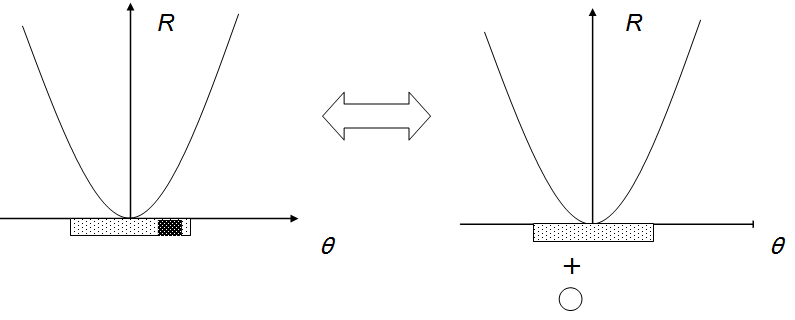
Figure 1: Stellar spot - point source equivalence. When viewed through the asymmetric filter that the instrument represents, a stellar spot is equivalent to a symmetrically placed virtual planet. $R$ is the interferometric coronagraphic transmission, and $\theta$ is angular sky position parameter.

3.4 Star Output

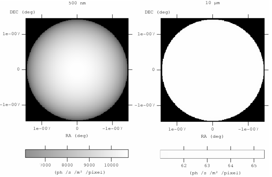
Figure 2: $209\times 209$-pixel Origin output images of a G0V star at 10 pc at wavelengths $\lambda=0.5\,\micro\mathrm{m}$ and $\lambda=10\,\micro\mathrm{m}$. Linear grayscales go from 0 to the maximum of brightness in each plot. The bandwidth of the channel is 1 $\micro\mathrm{m}$.

Taking into account the considerations presented in Sects. 3.1 through 3.3, the option chosen in our model is to generate a resolved image of the limb-darkened stellar surface with sufficient resolution to allow for a correct estimation of the leakage (Fig. 2). In order to avoid introducing too many settings in our model (which would prevent inspection of a wide range of possible scenarios), the only parameter considered to account for non-symmetric stellar contribution is the pointing error, i.e. a possible angular offset between the line of sight and the position of the star.

The images in Fig. 2, and a majority of the following, are outputs of the widely used fv (http://heasarc.nasa.gov/ftools/fv) Fits viewer and editor program, which is proposed as an interface for the ORIGIN software. This was preferred to a dedicated interface development, in order to use tools already familiar to the astrophysical community as much as possible.

4 Exoplanets

The exoplanets will be unresolved at the instrument’s resolution. The specific intensity of the $j$-th planet is therefore:

$$I_{j}(\mathbf{s},\lambda,t)=\Bigl{[}F_{\mathrm{e},j}(\lambda,t)+F_{\mathrm{r},j}(\lambda,t)\Bigr{]}\,\delta\Bigl{(}\mathbf{s}-\mathbf{s}_{j}(t)\Bigr{)}\,,$$ (19)

where $\delta$ is Dirac’s distribution, $\mathbf{s}_{j}(t)$ is the angular position of the planet at date $t$, $F_{\mathrm{e}}$ is the specific flux intrinsically emitted by the planet and $F_{\mathrm{r}}$ is the stellar flux reflected by the planet. Absorption of the planetary flux by exozodiacal dust, even in the case of edge-on systems, would assume a global dust density that would rule out nulling detection, so this is not implemented. The specific fluxes emitted and reflected by a given planet are discussed in the following section; we have, however, dropped the planet index $j$ for the sake of simplicity.

4.1 Planet Emission

The diversity of exoplanets is expected to be considerable, especially in the case of terrestrial planets (Gaidos & Selsis 2007). The composition of a given terrestrial exoplanet’s atmosphere, and thus its spectrum, will depend on many parameters. Among these parameters are the stellar type and the detailed chemical composition of its parent star, its orbital distance, its mass, its accretion history, the relative abundance of accreted solids (silicate, metal, ice) and volatiles (including water), the age of the system, and possibly, the existence of an extensive biosphere. Simulation of planetary atmospheres is a rather young field, and the encompassed models represent a level of complexity beyond the scope of this work. The best approach for an exoplanetary systems FOV model is to be able to use external spectra, provided by teams working on the computation of realistic synthetic spectra. A collection of identified object spectra is already available: phase-dependent Jupiter-like planets at different orbital distances (Barman et al. 2005), Earth, Mars or Venus-like planets and derived terrestrial planets (Selsis 2000; Schindler & Kasting 2000; Selsis et al. 2002; Des Marais et al. 2002; Tinetti et al. 2006, 2005), Earth-replicas orbiting around G, F, and K stars (Selsis 2000; Segura et al. 2003), M stars (Segura et al. 2005) the Earth throughout its history (Kaltenegger et al. 2007), Earth-like planets across the habitable zone (Paillet 2006), and ”ocean-planets” (Léger et al. 2004).

Alternatively, it is possible to implement a simple black body emission spectral energy distribution. In our model, its effective temperature can be either calculated upon a radiative equilibrium with the star, or fixed by the user. The effective temperature of the planet $T_{\mathrm{p}}$ derived from radiative equilibrium with the star is:

$$T_{\mathrm{p}}=(1-A_{\mathrm{p}})^{1/4}\,\sqrt{\frac{R_{\star}}{2\,r}}\,T_{\star}\,,$$ (20)

where $A_{\mathrm{p}}$ is the Bond albedo, and the distance $r$ from the planet to the star depends on the observation date $t$ and is computed by solving the orbital equations. If a simple black body emission is used, the emitted flux is

$$F_{\mathrm{e}}(\lambda,t)=\pi\,\left(\frac{R_{\mathrm{p}}}{d}\right)^{2}\,B_{\lambda}(T_{\mathrm{p}})\,,$$ (21)

where $B_{\lambda}$ is the Planck function.

4.2 Reflected Flux

Depending on their albedo and on their phase with respect to the observer, the planets partially reflect the flux of their hosting star. The specific flux received by a planet from its star, at a distance $r$ from the star is:

$$F_{\lambda}(r)=2\,\pi\,\left(\frac{R_{\star}}{r}\right)^{2}\,I^{\mathrm{n}}_{\lambda}\,Q_{\lambda}\,,$$ (22)

where the factor $Q_{\lambda}$ depends on the star limb-darkening law:

$$Q_{\lambda}=\int_{0}^{1}D_{\lambda}(\mu)\,\mu\,\mathrm{d}\mu\,.$$ (23)

The factor $Q_{\lambda}$ can be computed for the considered limb-darkening laws:

$$Q_{\lambda}=\left\{\begin{array}[]{ll}1/2&\mbox{\small(black body)}\\ (3-x_{\lambda})/6&\mbox{\small(linear law)}\\ (9-3\,x_{\lambda}+2\,y_{\lambda})/18&\mbox{\small(logarithmic law)}\\ (15-5\,x_{\lambda}-3\,y_{\lambda})/30&\mbox{\small(square-root law)}\\ \end{array}\right.$$ (24)

The flux reflected by the planet then is:

$$F_{\mathrm{r}}(\lambda,t)=\mathcal{R}(\lambda,\xi)\,\left(\frac{R_{\mathrm{p}}}{d}\right)^{2}\,F_{\lambda}(r)\,.$$ (25)

$F_{\lambda}(r)$ is the specific flux received by the planet from its hosting star as given by Eq. (22) and $d$ is its distance from the observer. $\mathcal{R}(\lambda,\xi)$ is the phase-dependent reflectivity of the planet, as seen at an angle $\xi$ from the star. This general expression of the reflectivity enables our model (which is open) to be updated with expressions taking into account specular reflection on a planet’s surface, as well as Mie and Rayleigh diffusion, which is beyond the scope of our present work. For now, we have used a Lambertian model $Ref(\lambda,\xi)=A_{\lambda}\,\phi(\xi)$. $A_{\lambda}$ is a constant and $\phi(\xi)$ is the fraction of the planetary disk surface illuminated by the star as seen by the observer (phase):

$$\phi(\xi)=\frac{1}{2}\,\left[1+\sin(\pi-\xi)\right]=\frac{1}{2}\,\left[1+\sin(\nu(t)+\omega(t))\,\sin i\right]$$ (26)

where $i$ is the inclination of the orbit, $\nu$ is the true anomaly, and $\omega$ is the argument of the periastron of the considered planet at the time of observation.

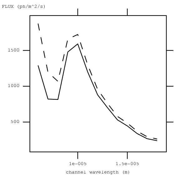
Figure 3: Full night side (solid) and full day side (dashed) emissions. Night: emission model of a 1.1 R_Jupiter planet of albedo 0.1, orbiting at 0.02 AU from parent star from Barman et al. (2005). Day: added full-disk reflection of Kurucz model 120 (G0V) stellar flux, from Van Hamme (1993). All seen at 10 pc. Channel width: 1 $\micro\mathrm{m}$.

Figure 3 exemplifies the importance of this phenomenon as simulated with our model. Actually, the emission spectrum of planets so close to their star is not uniform with their apparent phase (Harrington et al. 2006).

5 Other Sources

5.1 Local Zodiacal Cloud

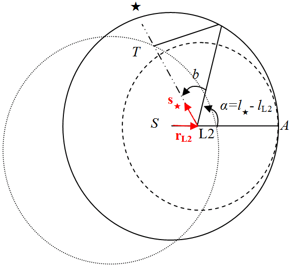
Figure 4: How the optical depth, for a target at a given ecliptical latitude $b$, increases with the target’s L2-relative ecliptical longitude $\alpha$ (S-Sun, L-L2 point(Sun - Earth), A-Antisolar direction, $l$-ecliptical longitude).

In order to compute the local zodiacal dust emission, we integrate along the line of sight (Fig. 4), from the observer’s location towards the target, through a 3-dimensional sampling of the Kelsall model (Kelsall et al. 1998). Our approach is thus similar to that of Landgraf & Jehn (2001), with some minor differences, and from a ”background drift”, fixed pointing direction perspective. Since there is no theoretical outer limit to the exponential law of the dust density in this model we integrate to the outer limit of the physical cloud; i.e. its collisional origin in the asteroid belt, at SA $\approx 5\,\mathrm{AU}$.

Given the size of the interferometer’s FOV, and with respect to the value of this outer limit, the local zodiacal flux contributes uniformly to the image. This is equivalent to a global noise level in the nulling data, depending only on the target’s sky position and on the instrument’s position at a given observation date.

Since scattering by dust is negligible compared to the thermal emission at 10 $\micro\mathrm{m}$, it can easily be seen that it is best, at a given mission time, to observe targets in the antisolar ecliptic meridian, because that is where the optical depth of the cloud is minimal. However, during spectroscopic observations, which can be 4 months long, the optical depth along the line of sight will vary.

Let $\mathbf{s}_{\star}$ be the direction of the target star (the time parameter $t$ is omitted for the sake of readability):

$$I_{\mathrm{z}}(\mathbf{s}_{\star},\lambda)=\int_{0}^{\mathrm{L2\,T}}J_{\mathrm{z}}(\mathbf{r}_{\mathrm{L2}}+u\,\mathbf{s}_{\star},\lambda)\,\mathrm{d}u$$ (27)

where the position $\mathbf{r}=\mathbf{r}_{\mathrm{L2}}+u\,\mathbf{s}_{\star}$ is relative to the Sun, $\mathbf{r}_{\mathrm{L2}}$ is the observer position, $u$ is the distance from the observer towards the source along the line of sight, and where $J_{\mathrm{z}}$ is the emitted specific intensity per unit of depth, i.e. the power emitted by the dust at position $\mathbf{r}$, per unit of volume, per unit of solid angle, per unit of spectral bandwidth, given by the model of Kelsall et al. (1998).

The direction of observation $\mathbf{s}_{\star}$ is $({RA},{DEC})$ in equatorial coordinates and, to perform the integration, it must be converted into ecliptic coordinates $(l,b)$.

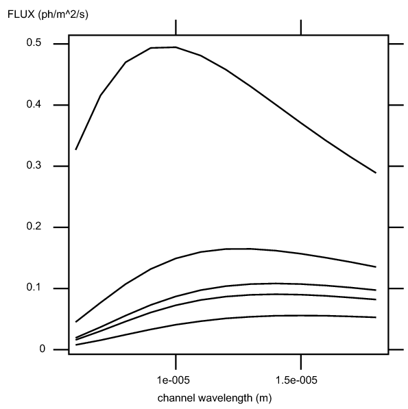
Figure 5: Local zodiacal cloud emission drift at L2 point over an evenly spread interval of 6 months, steadily increasing from the anti-solar direction (lowest) to solar (highest). The ecliptical latitude of the target is 10^∘, channel width is 1 $\micro\mathrm{m}$. FOV radius is $0\aas@@fstack{\prime\prime}6$.

Figure 5 shows the drift of the local zodiacal emission background, for a given target, from the L2 point, over a evenly spread period of 6 months. At around 14 $\micro\mathrm{m}$ the zodiacal drift over 3 months is 200%. Thus the global noise level drift is $\approx 14\,\%$ in that particular channel, over a duration not unlikely for a spectroscopic observation.

5.2 The Exozodiacal Cloud

In our model, we assume that the exozodiacal cloud dust has similar properties to the solar zodiacal cloud (Sect.  5.1), hence we simulate it by scaling the model of Kelsall et al. (1998). All parameters are free, enabling for instance to produce large clumps of dust useful for robustness testing of planet signal extraction algorithms.

5.3 Galactic Interstellar Medium

Emission levels.

Galactic interstellar medium (ISM) IR emission can reach hundreds of $\mathrm{MJy}\,\mathrm{sr}^{-1}$ in the infrared (Schlegel et al. 1998). Over the typical $0\aas@@fstack{\prime\prime}6$ field of view of interferometer, this equates to 2500 $\mathrm{ph}\,\mathrm{s}^{-1}\,\mathrm{m}^{-2}\,\micro\mathrm{m}^{-1}$ at 10 $\micro\mathrm{m}$. We carried out simulations on ESA code (den Hartog 2006), showing that the additional noise level provided by a such a background doubles the detection time of an exo-Earth.

We have therefore extracted from the Improved Reprocessing of the IRAS Survey (IRIS) maps (Miville-Deschênes & Lagache 2005) 12.5 and 25 $\micro\mathrm{m}$ background emission levels for the target list of Kaltenegger et al. (2006). Figure 6 shows the histogram for the emission at 12.5 $\micro\mathrm{m}$. Background emissions (again, over the FOV) do not exceed 900 $\mathrm{ph}\,\mathrm{s}^{-1}\,\mathrm{m}^{-2}\,\micro\mathrm{m}^{-1}$, with a mean value of $\sim 41$ and a median value of $\sim 32$.

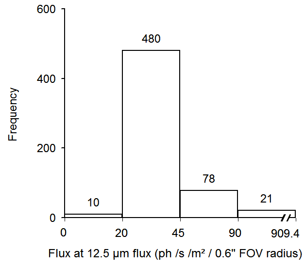
Figure 6: Histogram of galactic interstellar medium emission at 12.5 $\micro\mathrm{m}$, for 609 targets form Kaltenegger et al. (2006)

It is worth noting that the resolution of the IRIS maps is $3\aas@@fstack{\prime}8$. How do we know that in such a pixel, we do not include the flux of unresolved sources (galactic stars, background galaxies, etc.), thus overestimating the flux of the ISM that would actually be intercepted by the interferometer’s FOV? Typical star count values for magnitudes greater that 20 (K band) range from $3[\log N\mathrm{deg}^{-2}\,0.5\mathrm{mag}^{-1}]$ for the galactic disk (not in the galactic plane) according to Girardi et al. (2005) to 4.5 for the bulge (Rodgers et al. 1986); this is equivalent to 25-50 stars per 0.5 mag per IRIS pixel. We can therefore keep in mind that the values of the ISM we have extracted may be conservative. However, given the above-mentioned statistics on current candidate lists, we have not proceeded to implement this correction yet.

Spectral variability.

As can be derived from Verstraete et al. (2001, Fig. 1 therein), variations of the continuum emission of the ISM, around 18 $\micro\mathrm{m}$ and integrated over the $0\aas@@fstack{\prime\prime}6$ FOV of the instrument, can reach a photon noise contribution of 50 $\mathrm{ph}\,\mathrm{s}^{-1}\,\mathrm{m}^{-2}\,\micro\mathrm{m}^{-1}$. ISM background calibration is thus required for spectroscopy.

The reddening absorption due to interstellar molecular clouds between ourselves and the targets, given their relative proximity, is too faint to be a bias.

Variability over the FOV.

Diffuse background ISM structure studies have a resolution limit of 10″(Ingalls et al. 2004). As can be seen in Fig. 3 of this reference, extrapolation of the $\alpha=-3.5$ power law to the FOV spatial frequency ($0\aas@@fstack{\prime\prime}6\leftrightarrow 1.6\,\mathrm{arcsec}^{-1}$) leads to an extrapolated power level of $10^{-7}\,\mathrm{MJy}^{2}\,\mathrm{sr}^{-1}$, corresponding to a statistical flux variation amplitude over a $0\aas@@fstack{\prime\prime}6$ FOV of $10^{-9}\leavevmode\nobreak\$Jy at 24 $\micro\mathrm{m}$, or $6\times 10^{-4}\leavevmode\nobreak\ \mathrm{ph}\,\mathrm{s}^{-1}\,\mathrm{m}^{-2}\,\micro\mathrm{m}^{-1}$. This is comparable to the flux of an exo-Earth (typically $0.5\leavevmode\nobreak\ \mathrm{ph}\,\mathrm{s}^{-1}\,\mathrm{m}^{-2}\,\micro\mathrm{m}^{-1}$ at 10 $\micro\mathrm{m}$). The emission of the cold ISM at 10 $\micro\mathrm{m}$ should be even lower, so the variation of the ISM emission in the FOV should not be visible in the nulling data processing, at exo-Earth detection level. Finally, it can be noted that the parallax of the closest targets ($0\aas@@fstack{\prime\prime}2$) is only a fraction of the FOV, so there should be no galactic ISM background drift with the parallax.

5.4 Faint Background Objects

Figure 7 displays an integration of a previously established galaxy count histogram (Lagache et al. 2004). As mentioned above, an exo-Earth at 10 pc emits $0.5\leavevmode\nobreak\ \mathrm{ph}\,\mathrm{s}^{-1}\,\mathrm{m}^{-2}\,\micro\mathrm{m}^{-1}$ at 10 $\micro\mathrm{m}$. We see that, statistically, there should be 0.01 objects brighter than that in a $0\aas@@fstack{\prime\prime}6$ FOV.

Figure 7: Integrated field galaxy counts. Plot has similar profile at 60 and 170 $\micro\mathrm{m}$, with maximums steadily decreasing with the wavelength.

In order to examine galactic stars in the FOV, we can investigate further the reference cited in Sect. 5.3 (Girardi et al. 2005, Fig. 6 therein). Let us consider the star count peak in the K band (2 $\micro\mathrm{m}$, longest wavelength available in this reference; in the FOV, that represents 2.2 $\times\leavevmode\nobreak\ 10^{-5}$ objects per 0.5 mag bandwidth, so it is not even necessary to consider the integrated count. We conclude that it is unlikely that one will encounter background stars emitting at the level of an exo-Earth or greater in the FOV. Were faint background objects still to occur in the FOV, they could be easily ruled out spectroscopically, and by monitoring their orbital motion during revisits.

In addition to the final remark of Sect. 5.3 concerning the ISM emission, the numbers above remain negligible if an extended FOV (taking into account the parallax) is considered instead, so we have not accounted for time variability of $I_{\mathrm{bg}}$ (galactic background drift).

Because of the above, our model does not specifically implement FOV background stars or galaxies.

6 Discussion

It is interesting to consider whether one or several of the source features identified above was already an “astrophysical limitation” in achieving the scientific objective of these exo-Earth finding missions. We recall that FOV source features where screened on the intuitive criterion whereby “anything producing a signal at the level of an exo-Earth deserves modeling”, in the prospect of full end-to-end testing simulations.

Currently, target catalogs for these survey missions have been started; for now, these are based on astrobiological interest and the few informed astro-engineering requirements available today, such as the existence of a secondary star too near and bright (Kaltenegger et al. 2006). Surveys of exozodiacal dust levels of nearby stars are planned or in progress; the statistics of this unknown parameter alone may impose dramatic revision of the scale and cost of missions, even though elements in favor of optimism do exist (Beichman et al. 2006).

In this context, the features of the sources described here are, in most cases, an order of magnitude below the exozodiacal cloud issue. Beyond the classical limitation of shot noise from unsought-for sources, additional requirements on the integration time (hence on the cost) may arise from signal processing specificities, such as systematic multiple planet signal disentangling, regardless of their relative positions and kinematics. This is the purpose of our ongoing work.

7 Summary

We have defined a FOV physical model of exoplanetary system scenes, and proposed an associated Fits input and output format. The input format is a tentative standard for defining exoplanetary systems. The output format is an input format for exoplanet seeking instrumental simulators. They are both described in the Appendices.

Submitting a fixed resolution image to an instrumental simulator is not practical, given the dynamics in resolution and flux between the various typical sources. The output flux is modeled by a “layering” of various sources (star, planets, dust). Each “layer” is of one type among i) a 3-D spectral flux image (for resolved sources), ii) a spectral flux and a position (for unresolved sources), iii) a FOV-uniform spectral contribution. For each source we have examined the detectable features that need to be modeled.

Depending on the spectral type of the parent star and of the wavelength, omitting to model limb-darkening is shown to induce a bias in the estimation of the leakage noise of up to $\sim 35\,\%$. Stellar spots produce a fainter signal than that of an exo-Earth. Local zodiacal drift is found to be smaller than 14 % in any given spectral channel. Galactic ISM background for a current list of $\sim 600$ targets peaks at $900\,\mathrm{ph}\,\mathrm{s}^{-1}\,\mathrm{m}^{-2}\,\micro\mathrm{m}^{-1}$, with a mean value of $\sim 41$ and a median value of $\sim 32$ for a typical FOV of $0\aas@@fstack{\prime\prime}6$. Simulations show that a doubling of the detection time of an exo-Earth is induced by a $2500\,\mathrm{ph}\,\mathrm{s}^{-1}\,\mathrm{m}^{-2}\,\micro\mathrm{m}^{-1}$ galactic emission background (compared to no background emission, this is the order of magnitude of the highest emissions). Finally, background galactic stars and distant galaxies as bright as, or brighter than an exo-Earth are unlikely in the FOV, even extended by parallax drift.

The model specifications have been embedded by Starlab & Thales Alenia Space (formerly Alcatel Alenia Space, see acknowledgments) into a Java simulator called Origin, soon to be open-source, using the input/output definition standards detailed in the Appendices. We are in the process of building upon this work to obtain an end-to-end simulation approach.

Appendix A Input format

We have developed a Fits (Hanisch et al. 2001) standard specifying the input parameters for modeling an exoplanetary system. This format takes advantage of the building block structure of Fits files. This building block approach also enables modular storage of stereotypes, as well as the possibility of linking to exterior databases in the future.

A.1 Overview and Primary HDU

All the data necessary to define a FOV (that can be read by flux calculators such as the Origin software – Sect. 7) are stored in a Fits file. Databases, such as chromatic specific intensities of bodies, are stored in Fits binary tables (i.e., with XTENSION=’BINTABLE’), whereas scalar parameters are stored in the headers of the extensions. The primary Header Data Unit (HDU) of an Origin input data file is informational only and contains no data. An example of such a primary HDU is provided in Table 4.

An Origin input data file provides the following HDUs:

• general scenario parameters (spectral channels, observation epoch, duration of the observation and number of snapshots to be produced during that time frame, FOV resolution and sizes),

• star parameters,

• local and exozodiacal cloud parameters,

• planet(s) parameters.

The order of HDUs is irrelevant, the file contains at most one HDU of each type (except for planets). HDUs are identified by their names (value of EXTNAME Fits keyword). Table 5 lists the different Fits extensions (actually Fits binary tables) used to implement the Origin input file format. The revision number of the Origin input file format described in this document is EXTVER=1 and is indicated by the value of Fits keyword EXTVER in each HDU extension. The various extensions used in Origin input data files are detailed in the subsequent subsections.

Table 4: Example of the header part of a primary HDU in an Origin input file.

SIMPLE  =                    T / true FITS file (http://fits.gsfc.nasa.gov/)
BITPIX  =                    8 / 8-bit twos complement binary unsigned integer
NAXIS   =                    0 / this HDU contains no data
EXTEND  =                    T / this file may contain FITS extensions
BLANK
COMMENT This is an input FITS file for ORIGIN software for exoplanetary
COMMENT system sky energy distribution modeling.
BLANK
HISTORY Created by SOMEBODY on SOMEDATE.
END

Table 5: Description of Fits extensions of Origin input file format. All these extensions are saved into a Fits binary table identified by its name, which is the value of the keyword EXTNAME. Column Number indicates the number of extensions of a given type allowed in the file.

Extension Name	Number	Description
’SCENARIO’	1	global parameters
’STAR’	1	star parameters
’EXO-ZODI’	1	exozodiacal cloud parameters
’LOCL-ZODI’	1	local zodiacal cloud parameters
’UNRESOLVED’	any	parameters for planets
	or other point-
	like objects

A.2 Scenario Table

The parameters defining the scenario of an exoplanetary system observation are stored into a Fits extension named ’SCENARIO’. The corresponding binary table contains a first column with the central wavelength of the channels, and a second with their width. A number of scalar parameters are also provided in the header part of this HDU:

• The value of L2-FLAG specifies whether the observer’s position is at the L2 point (see Sect. 2.2). Otherwise, Earth position is assumed.

• The value of DW-EPOCH is the Julian date of the beginning of the operational phase of the instrument, as an epoch that later mission events will be relative to (DW comes from Darwin, the mission for which this standard was initially developed).

• The value of OBS-DATE is the time (in fractional JD) from DW-EPOCH when the current observation starts. Origin uses compact computer algorithms by Fliegel & van Flandern (1968) for converting between Julian days and Gregorian calendar dates.

• The value of OBS-STEP is the duration between two successive snapshot outputs of the scene, for following orbital motion of planets.

• STR-RES is the resolution at which the flux calculator (as the Origin software) generates a chromatic sky energy distribution (an image cube) of the star.

• IMG-RES and IMG-FOV are the resolution and FOV, respectively, of the image (cube) of the exozodiacal dust. Also, IMG-FOV is used to compute the FOVs solid angle for uniform contribution calculation (see Sect. B.4).

• CLOUD-DZ is the integration step along the line of sight through 3-D dust distributions.

These parameters are listed in Table 6. Table 7 shows a typical SCENARIO header of an Origin input file. Note that, in this header, the value of NAXIS2 is also the number of effective spectral channels for which output will be generated. The columns of the binary table in a SCENARIO extension are listed in Table 8.

Table 6: List of Fits keywords used to define scalar parameters of the ’SCENARIO’ extension.

Keyword	Description	Units
L2-FLAG	observer at L2 point
DW-EPOCH	date of beginning of mission	JD
OBS-DATE	observation date (from DW-EPOCH)	JD
OBS-STEP	time between 2 snapshot outputs	hrs
OBS-NB	number of snapshot outputs
STR-RES	star resolution	″
IMG-RES	resolution of the zodiacal image	″
IMG-FOV	FOV	″
CLOUD-DZ	z integration step through cloud	AU

Table 7: Typical SCENARIO header in an Origin input file.

XTENSION= ’BINTABLE’           / FITS 3D BINARY TABLE
BITPIX  =                    8 / Binary data
NAXIS   =                    2 / Table is a matrix
NAXIS1  =                   16 / Width of table in bytes
NAXIS2  =                   13 / Number of entries in table
PCOUNT  =                    0 / Random parameter count
GCOUNT  =                    1 / Group count
TFIELDS =                    2 / Number of fields in each row
EXTNAME = ’SCENARIO’           / Table name
EXTVER  =                    1 / Version number of table
TFORM1  = ’D       ’           / Data type for field
TTYPE1  = ’SPCH-CWL’           / Label for field
TUNIT1  = ’m       ’           / Physical units for field
TFORM2  = ’D       ’           /  Data type for field
TTYPE2  = ’SPCH-WDT’           / Label for field
TUNIT2  = ’m       ’           / Physical units for field
L2-FLAG = ’F       ’           / Observer at L2 point?
DW-EPOCH=              2456000 / Beginning of mission, JD
OBS-DATE=                  100 / Beginning of observation, from DW-EPOCH
OBS-STEP=                   24 /
OBS-NB  =                    1
STR-RES =                 8E-6
IMG-FOV =                0.715
IMG-RES =                 0.01
ORB-FOV =                    2
ORB-RES =                 0.01
CLOUD-DZ=                  0.1 / added AU
END

Table 8: Description of Fits binary table for the scenario extension of the Origin input file format.

Column	Description	Units
SPCH-CWL	central wavelength of channels	m
SPCH-WDT	bandwidths of channels	m

A.3 Star Parameters

The star model parameters are stored in a ’STAR’ extension. Table 9 lists the keywords of the star model.

Table 9: Star model keywords.

symbol	description	units
ICRS- ALP, BET	ICRS star coordinates	deg
SHIFT- ALP, BET	offset of the star image from the pointing direction of the instrument	deg
SP-MODE	whether black body or provided spectrum should be used	flag
LIMB-DRK	which (uniform, linear, quadratic, etc.) limb darkening law should be used	flag
RLT-FLAG	which among luminosity, star radius or effective temperature should be calculated from the others	flag
MGR	which among mass, surface gravity or radius should be calculated from the others	flag
ML	which from mass or luminosity should be calculated from the other	flag
DISTANCE	distance from observer	pc
EFF-TEMP	star effective temperature	$\hbox{${}^{\circ}$}\mathrm{K}$
MASS	mass of the star	$M_{\odot}$
LUMINOSI	star luminosity	$L_{\odot}$
RADIUS	star radius	$R_{\odot}$
LOG-GRAV	log of star surface gravity	$g_{\odot}$

Origin provides a database of monochromatic limb-darkening parameters and specific intensity for stars of various spectral type and luminous class (see Sect. 3.1). This database is built from Van Hamme (1993) tables and from a model of the HR diagram of existing stars, to establish the relation between spectral type and luminosity class, and physical parameters such as the star’s effective temperature, surface gravity and luminosity. Tables 10 displays, for reference, the mean specific intensity in photometric bands, for the spectral types of stars envisioned for exoplanet search.

Table 10: Mean specific intensity in photometric bands (units: $\mathrm{ph}\,\mathrm{s}^{-1}\,\mathrm{m}^{-2}\,\mathrm{sr}^{-1}\,\micro\mathrm{m}^{-1}$).

Type	U	B	V	R	I	J	H	K	L	M	N	Q
F0V	$1.5\cdot 10^{26}$	$2.6\cdot 10^{26}$	$2.4\cdot 10^{26}$	$1.8\cdot 10^{26}$	$1.2\cdot 10^{26}$	$7.1\cdot 10^{25}$	$3.9\cdot 10^{25}$	$1.9\cdot 10^{25}$	$5.5\cdot 10^{24}$	$1.8\cdot 10^{24}$	$2.4\cdot 10^{23}$	$3.9\cdot 10^{22}$
F2V	$1.3\cdot 10^{26}$	$2.2\cdot 10^{26}$	$2.1\cdot 10^{26}$	$1.6\cdot 10^{26}$	$1.1\cdot 10^{26}$	$6.7\cdot 10^{25}$	$3.7\cdot 10^{25}$	$1.8\cdot 10^{25}$	$5.4\cdot 10^{24}$	$1.8\cdot 10^{24}$	$2.3\cdot 10^{23}$	$3.7\cdot 10^{22}$
F5V	$8.6\cdot 10^{25}$	$1.5\cdot 10^{26}$	$1.6\cdot 10^{26}$	$1.3\cdot 10^{26}$	$9.6\cdot 10^{25}$	$5.8\cdot 10^{25}$	$3.4\cdot 10^{25}$	$1.7\cdot 10^{25}$	$5.0\cdot 10^{24}$	$1.6\cdot 10^{24}$	$2.1\cdot 10^{23}$	$3.5\cdot 10^{22}$
F8V	$6.7\cdot 10^{25}$	$1.2\cdot 10^{26}$	$1.3\cdot 10^{26}$	$1.1\cdot 10^{26}$	$8.7\cdot 10^{25}$	$5.4\cdot 10^{25}$	$3.3\cdot 10^{25}$	$1.6\cdot 10^{25}$	$4.8\cdot 10^{24}$	$1.5\cdot 10^{24}$	$2.0\cdot 10^{23}$	$3.3\cdot 10^{22}$
G0V	$5.1\cdot 10^{25}$	$9.6\cdot 10^{25}$	$1.1\cdot 10^{26}$	$1.0\cdot 10^{26}$	$7.8\cdot 10^{25}$	$5.0\cdot 10^{25}$	$3.1\cdot 10^{25}$	$1.5\cdot 10^{25}$	$4.6\cdot 10^{24}$	$1.5\cdot 10^{24}$	$2.0\cdot 10^{23}$	$3.2\cdot 10^{22}$
G2V	$3.7\cdot 10^{25}$	$7.5\cdot 10^{25}$	$9.3\cdot 10^{25}$	$8.6\cdot 10^{25}$	$6.9\cdot 10^{25}$	$4.6\cdot 10^{25}$	$3.0\cdot 10^{25}$	$1.4\cdot 10^{25}$	$4.4\cdot 10^{24}$	$1.4\cdot 10^{24}$	$1.9\cdot 10^{23}$	$3.1\cdot 10^{22}$
G5V	$3.7\cdot 10^{25}$	$7.5\cdot 10^{25}$	$9.3\cdot 10^{25}$	$8.6\cdot 10^{25}$	$6.9\cdot 10^{25}$	$4.6\cdot 10^{25}$	$3.0\cdot 10^{25}$	$1.4\cdot 10^{25}$	$4.4\cdot 10^{24}$	$1.4\cdot 10^{24}$	$1.9\cdot 10^{23}$	$3.1\cdot 10^{22}$
G8V	$2.5\cdot 10^{25}$	$5.7\cdot 10^{25}$	$7.6\cdot 10^{25}$	$7.4\cdot 10^{25}$	$6.0\cdot 10^{25}$	$4.2\cdot 10^{25}$	$2.8\cdot 10^{25}$	$1.4\cdot 10^{25}$	$4.2\cdot 10^{24}$	$1.3\cdot 10^{24}$	$1.8\cdot 10^{23}$	$2.9\cdot 10^{22}$
K0V	$1.7\cdot 10^{25}$	$4.3\cdot 10^{25}$	$6.0\cdot 10^{25}$	$6.1\cdot 10^{25}$	$5.2\cdot 10^{25}$	$3.8\cdot 10^{25}$	$2.6\cdot 10^{25}$	$1.3\cdot 10^{25}$	$4.0\cdot 10^{24}$	$1.2\cdot 10^{24}$	$1.7\cdot 10^{23}$	$2.8\cdot 10^{22}$
K1V	$1.0\cdot 10^{25}$	$3.1\cdot 10^{25}$	$4.7\cdot 10^{25}$	$5.0\cdot 10^{25}$	$4.4\cdot 10^{25}$	$3.4\cdot 10^{25}$	$2.5\cdot 10^{25}$	$1.2\cdot 10^{25}$	$3.8\cdot 10^{24}$	$1.1\cdot 10^{24}$	$1.6\cdot 10^{23}$	$2.7\cdot 10^{22}$
K2V	$1.0\cdot 10^{25}$	$3.1\cdot 10^{25}$	$4.7\cdot 10^{25}$	$5.0\cdot 10^{25}$	$4.4\cdot 10^{25}$	$3.4\cdot 10^{25}$	$2.5\cdot 10^{25}$	$1.2\cdot 10^{25}$	$3.8\cdot 10^{24}$	$1.1\cdot 10^{24}$	$1.6\cdot 10^{23}$	$2.7\cdot 10^{22}$
K3V	$6.0\cdot 10^{24}$	$2.1\cdot 10^{25}$	$3.4\cdot 10^{25}$	$4.0\cdot 10^{25}$	$3.7\cdot 10^{25}$	$3.0\cdot 10^{25}$	$2.3\cdot 10^{25}$	$1.2\cdot 10^{25}$	$3.6\cdot 10^{24}$	$1.1\cdot 10^{24}$	$1.5\cdot 10^{23}$	$2.5\cdot 10^{22}$
K4V	$3.2\cdot 10^{24}$	$1.4\cdot 10^{25}$	$2.4\cdot 10^{25}$	$3.1\cdot 10^{25}$	$3.0\cdot 10^{25}$	$2.6\cdot 10^{25}$	$2.2\cdot 10^{25}$	$1.1\cdot 10^{25}$	$3.4\cdot 10^{24}$	$9.9\cdot 10^{23}$	$1.5\cdot 10^{23}$	$2.4\cdot 10^{22}$
K5V	$1.6\cdot 10^{24}$	$8.1\cdot 10^{24}$	$1.6\cdot 10^{25}$	$2.2\cdot 10^{25}$	$2.4\cdot 10^{25}$	$2.2\cdot 10^{25}$	$2.0\cdot 10^{25}$	$1.0\cdot 10^{25}$	$3.2\cdot 10^{24}$	$9.2\cdot 10^{23}$	$1.4\cdot 10^{23}$	$2.3\cdot 10^{22}$
K7V	$7.6\cdot 10^{23}$	$4.4\cdot 10^{24}$	$9.9\cdot 10^{24}$	$1.5\cdot 10^{25}$	$1.8\cdot 10^{25}$	$1.8\cdot 10^{25}$	$1.7\cdot 10^{25}$	$8.8\cdot 10^{24}$	$2.9\cdot 10^{24}$	$8.6\cdot 10^{23}$	$1.3\cdot 10^{23}$	$2.2\cdot 10^{22}$
M0V	$3.9\cdot 10^{23}$	$2.3\cdot 10^{24}$	$5.8\cdot 10^{24}$	$9.6\cdot 10^{24}$	$1.3\cdot 10^{25}$	$1.4\cdot 10^{25}$	$1.3\cdot 10^{25}$	$7.4\cdot 10^{24}$	$2.6\cdot 10^{24}$	$8.0\cdot 10^{23}$	$1.3\cdot 10^{23}$	$2.1\cdot 10^{22}$
M1V	$3.9\cdot 10^{23}$	$2.3\cdot 10^{24}$	$5.8\cdot 10^{24}$	$9.6\cdot 10^{24}$	$1.3\cdot 10^{25}$	$1.4\cdot 10^{25}$	$1.3\cdot 10^{25}$	$7.4\cdot 10^{24}$	$2.6\cdot 10^{24}$	$8.0\cdot 10^{23}$	$1.3\cdot 10^{23}$	$2.1\cdot 10^{22}$
M2V	$1.8\cdot 10^{23}$	$1.2\cdot 10^{24}$	$3.2\cdot 10^{24}$	$5.5\cdot 10^{24}$	$9.4\cdot 10^{24}$	$1.1\cdot 10^{25}$	$1.1\cdot 10^{25}$	$6.2\cdot 10^{24}$	$2.3\cdot 10^{24}$	$7.3\cdot 10^{23}$	$1.2\cdot 10^{23}$	$2.0\cdot 10^{22}$
M3V	$1.8\cdot 10^{23}$	$1.2\cdot 10^{24}$	$3.2\cdot 10^{24}$	$5.5\cdot 10^{24}$	$9.4\cdot 10^{24}$	$1.1\cdot 10^{25}$	$1.1\cdot 10^{25}$	$6.2\cdot 10^{24}$	$2.3\cdot 10^{24}$	$7.3\cdot 10^{23}$	$1.2\cdot 10^{23}$	$2.0\cdot 10^{22}$
M4V	$1.7\cdot 10^{23}$	$1.1\cdot 10^{24}$	$3.2\cdot 10^{24}$	$5.7\cdot 10^{24}$	$9.5\cdot 10^{24}$	$1.1\cdot 10^{25}$	$1.0\cdot 10^{25}$	$6.1\cdot 10^{24}$	$2.3\cdot 10^{24}$	$7.4\cdot 10^{23}$	$1.2\cdot 10^{23}$	$2.0\cdot 10^{22}$

The star model can be built by choosing one of the items from the stellar database provided with the Origin software, or by specifying the star parameters (either in the same format as the database or, more simply, by a simple black body emission model characterized by the star effective temperature, luminosity or radius, mass or surface gravity and, optionally, limb-darkening parameters).

A.4 (Exo)zodiacal Cloud

Exo- and local zodiacal cloud parameters are stored into EXTNAME=’EXO-ZODI’ and EXTNAME=’LOCAL-ZODI’ extensions. Table 11 lists the keywords of the (exo)zodiacal model. Most parameters are those of the implemented Kelsall et al. (1998) model. The binary table of these extensions list solar system’s Kelsall et al. (1998) parameters of the three dust bands of the zodiacal cloud.

Table 11: (Exo)zodiacal model keywords.

symbol	description	units
TYPE	whether this extension is a local or exo- zodiacal cloud	flag
ZODI	mean density of dust	zodi
DUST-ST	dust sublimation temperature	$\hbox{${}^{\circ}$}\mathrm{K}$
DUST-RT	dust reference temperature	$\hbox{${}^{\circ}$}\mathrm{K}$
ETL	exponent temperature law coefficient	unitless
CLOUD-O	cloud outer radius	AU
SC-*	smooth cloud parameters of the Kelsall model, not all listed here

A.5 Unresolved Sources

Extension(s) EXTNAME=’UNRESOLVED’ store the parameters for unresolved sources such as planets. The format allows the specification of all their orbital parameters, but can also be used to account for fixed background point-like sources such as field stars or distant galaxies. Table 12 lists the keywords of the unresolved sources model. In addition to these, Kelsall et al. (1998) parameters of the circumsolar dust ring and blob can be specified. Origin uses the Kelsall et al. (1998) model equations, except the radius of the ring is the semi-major axis of the planet. Table 13 lists the columns of the binary table of the unresolved source extension: this is the optionally provided planetary spectrum.

Table 12: Unresolved sources (planets) model keywords.

symbol	description	units
ORB-APER	which, from semi-major axis or period is computed from the other	flag
P-RADIUS	planet radius	$R_{\oplus}$
P-TEMP	planet temperature	$\hbox{${}^{\circ}$}\mathrm{K}$
P-ALBEDO	planet albedo	unitless
ORB-T0	epoch of periastron passage	Julian date
ORB-OMA	position angle of the ascending node	deg
ORB-OMP	argument of periastron	deg
ORB-I	inclination of orbit	deg
ORB-E	eccentricity	unitless
ORB-A	semi-major axis	AU
ORB-PER	orbital period	days
SP-FLAG	whether to use specific intensities provided in the extensions binary table, or black body emission	flag

Table 13: Description of Fits binary table for unresolved extension in the Origin input file format.

Column	Description	Units
LAMBDA	channel’s central wavelength	m
SP_FLUX	specific intensity	ph s-1 m-2 sr-1 $\micro\mathrm{m}$ -1

Appendix B Output Format

The output format of the Origin software is also proposed as an input standard for instrumental simulators. It consists of two Fits files (or two series of files, if several observations at different times are demanded). The ORBIT file simply contains an image of the planets’ orbits with the current position of each planet, and it mainly serves a human visual check purpose. The LAYERED file contains the physical information that an instrumental simulator needs, and is described in the following.

We first note that the dynamic in specific intensity and resolution between the different sources in a planetary system scene is such that it is impractical to compute a global image, with a given resolution, of the whole FOV, and submit it to an instrumental simulator. Following the input standard, the output is also layered, as a Fits file containing three types of descriptions of incoming fluxes: resolved sources, unresolved sources, and FOV-uniform contributions, that can all be used by an instrumental simulator.

These files, being generated by the Origin software, are quite explicit, so this section is considerably more straightforward than the previous.

B.1 Primary HDU

Unlike the input format, the primary HDU restates some of the data from the input format. Table 14 gives an example of such a header.

Table 14: Typical primary header in an Origin output file.

SIMPLE  =                    T / Java FITS: Mon May 22 07:38:11 CEST 2006
BITPIX  =                    8
NAXIS   =                    0 / Dimensionality
EXTEND  =                    T / file contains FITS extensions
COMMENT = ’ORIGIN LAYERED OUTPUT FILE’ /
ORIGIN  = ’ORIGIN v1.0’        / Name and version of software
AUTHOR  = ’Author  ’           /
DATE    = ’Mon May 22 07:38:10 CEST 2006’ / File creation date
CTRLFILE= ’C:\ORIGIN\Livraison\Full Scenarii\Gl_876.fits’ / Name and path of ORI
DW-EPOCH=            2456000.0 / Darwin epoch [JD]
OBS-DATE=                100.0 / Observation date since epoch [days]
IMG-NBR =                    6 / Number of images generated during simulation
IMG-RANK=                    1 / Rank of current image simulation
END

B.2 Output Spectral Channels

In the output file, the EXTNAME=’SPCHANNELS’ extension is a binary table which gives the effective central wavelengths and spectral bandwidths of the simulated model. This information is similar to that specified in the input format (see Sect. A.2), and is not further described here.

B.3 Star or Exo-zodiacal Output Maps

In the output file, the EXTNAME=’RESOLVED OBJECT LAYER’ extensions are Fits images containing 3-D maps (right ascension, declination and wavelength) of the star’s limb darkened photosphere, or of the exozodiacal dust cloud. Table 15 shows an example of the header of this extension. The number of pixels in the image is always odd, with the reference pixel marking the center of the image. For an image example, refer to Fig. 2.

Table 15: Typical ’RESOLVED OBJECT LAYER’ header in an Origin output file.

XTENSION= ’IMAGE   ’           / Java FITS: Wed Mar 15 10:35:36 CET 2006
BITPIX  =                  -64
NAXIS   =                    3 / Dimensionality
NAXIS1  =                  121
NAXIS2  =                  121
NAXIS3  =                   13
PCOUNT  =                    0 / No extra parameters
GCOUNT  =                    1 / One group
EXTNAME = ’RESOLVED OBJECT LAYER’/This Layer contains the star image
EXTVER  =                    1 /
CTYPE1  = ’RA      ’           / Right ascension axis
CRPIX1  =                   61 / Reference pixel along axis 1 (starting from 1)
CRVAL1  =                 75.0 / Coordinate of ref. pixel along axis 1 [deg]
CDELT1  = -2.222222222222222E-9/ Pixel step along axis 1 [deg]
CTYPE2  = ’DEC     ’           / Declination axis
CRPIX2  =                   61 / Reference pixel along axis 2 (starting from 1)
CRVAL2  =                155.0 / Coordinate of ref. pixel along axis 2 [deg]
CDELT2  = 2.222222222222222E-9 / Pixel step along axis 2 [deg]
END

B.4 Local Zodiacal and Galactic Background

The background emission of the local zodiacal light, which is uniform over the field of view, is provided by the output format in $\mathrm{ph}\,\mathrm{s}^{-1}\,\mathrm{m}^{-2}$ per spectral channel in the binary table extension EXTNAME=’CONSTANT LAYER’ (Fig. 5). For that, the Origin software considers the FOV solid angle defined in the EXOZODI extension in the input format (see Sect. A.2). The header of this extension contains only the binary tables column definitions (Table 16).

Table 16: Description of Fits binary table columns for constant layer extension in the Origin output file format.

Column	Description	Units
SPCHCWL	channel’s central wavelength	m
SPCHWDT	channel’s width	m
SPCHFLUX	flux	ph s-1 m-2

The galactic background can be manually inserted here using this same extension format, since it requires no calculation by the Origin software.

B.5 Planets

The output file format contains as many UNRESOLVED OBJECT LAYER binary table extensions as there were UNRESOLVED planet definition extensions in the corresponding input file. Table 17 shows the header of such a planet binary table output extension. It provides the precise coordinates in the field of view of the unresolved source (fields RA-STR and DEC-STR). The binary table itself contains the calculated flux for the planet, degraded to the resolution indicated by the primary extension (Sect. B.1). It can be seen that the columns of this table are exactly the same as those of the CONSTANT LAYER extension (Sect. B.4 and Table 16).

Table 17: Typical ’UNRESOLVED’ header in an Origin output file.

XTENSION= ’BINTABLE’           / Java FITS: Wed Mar 15 10:35:43 CET 2006
BITPIX  =                    8
NAXIS   =                    2 / Dimensionality
NAXIS1  =                   24
NAXIS2  =                   13
PCOUNT  =                    0
GCOUNT  =                    1
TFIELDS =                    3
TFORM1  = ’1D      ’
TDIM1   = ’(1)     ’
TFORM2  = ’1D      ’
TDIM2   = ’(1)     ’
TFORM3  = ’1D      ’
TDIM3   = ’(1)     ’
EXTNAME = ’UNRESOLVED OBJECT LAYER’/This Layer contains the spectrum of a planet
EXTVER  =                    1 /
RA      =    75.00005875513867 / Object Absolute Right Ascension [deg]
DEC     =    155.0001242618757 / Object Absolute Declination [deg]
RA-STR  =  0.21151849913006165 / Object Right Ascension from Star [Arcsec]
DEC-STR =   0.4473427524966594 / Object Declination from Star [Arcsec]
TTYPE1  = ’SPCHCWL ’           / Spectral channel central wavelength
TUNIT1  = ’m       ’           /
TTYPE2  = ’SPCHWDT ’           / Spectral channel width
TUNIT2  = ’m       ’           /
TTYPE3  = ’SPFLUX  ’           / Object Flux
TUNIT3  = ’count/m^2/s’        /
END