On Axial and Plane–Mirror Inhomogeneities in the WMAP3 Cosmic Microwave Background Maps

Abstract. We study inhomogeneities in the distribution of the excursion sets in the Cosmic Microwave Background (CMB) temperature maps obtained by the three years survey of the Wilkinson Microwave Anisotropy Probe (WMAP). At temperature thresholds $|T|<90\mu K$, the distributions of the excursion sets with over 200 pixels are concentrated in two regions, nearly at the antipodes, with galactic coordinates $l=94^{\circ}.7,\,b=34^{\circ}.4$ and $l=279^{\circ}.8,\,b=-29^{\circ}.2$. The centers of these two regions drift towards the equator when the temperature threshold is increased. The centers are located close to one of the vectors of $\ell=3$ multipole. The two patterns of the substructures in the distribution of the excursion sets are mirrored, with $\chi^{2}=0.7-1.5$. There is no obvious origin of this effect in the noise structure of WMAP, and there is no evidence for a dependence on the galactic cut. Would this effect be cosmological, it could be an indication of an anomalously large component of horizon-size density perturbations, independent of one of the spatial coordinates, and/or of a non-trivial slab-like spatial topology of the Universe.

1 Introduction

The power spectrum of CMB has provided essential information on the cosmological parameters [1, 2]. Another important source of information are CMB temperature maps which are particularly useful for the study of possible non-Gaussianity signals of various nature. Among the latter are the alignments of low multipoles, claimed as anomalous with respect to Gaussian distribution (e.g. [3, 4, 5, 6, 7, 8, 9]). In the present paper we analyse axial inhomogeneities in the distribution of the excursion sets in the WMAP3 maps; these can be related to the alignments mentioned above. We have estimated the centers of excursion sets at given temperature thresholds and for a given pixel count. The distribution of the centers of the excursion sets revealed inhomogeneities, with mirroring features, which we analyse below. Though the Galactic and interplanetary contamination can be the major contributor here, and hence the non-cosmological nature of the low multipoles, we nevertheless discuss briefly the principal conditions for arising of the mirroring from topological properties of the Universe.

2 Excursion sets

For this analysis we used the 94 GHz (3.2mm) WMAP 3-year maps. These maps feature the highest angular resolution, and are less polluted than lower frequency channels by synchrotron radiation of our Galaxy. The $|b|<20^{o}$ region has been excluded as usual, to minimize effects due to the Galactic disk.

The algorithm for defining of the center of the pixelized excursion sets, and of their other parameters, has been described in [10, 11]; temperature independent ellipticity in the excursion sets was found in Boomerang’s and WMAP’s maps, and had been found in the COBE maps as well [12]. The algorithm is based on Cartan’s proof that maximally compact subgroups of Lie groups are always conjugate [13], i.e. due to the conditions of existence of the center of mass of the given set of points. For Riemannian manifolds the center of mass of the points $\{x_{i}\},i=1,...,n$ is defined as

$$x=\frac{1}{n}(x_{1}+x_{2}+...+x_{n}),$$ (1)

or that the mass center is the point where the following function is minimized:

$$y\rightarrow\sum_{1}^{n}d(x,x_{i})^{2}.$$ (2)

Though for present purposes the temperature weighting is not important, this procedure in principle enables such generalization assigning a weight $T_{i}$ to each pixel of coordinate $x_{i}$.

Without loosing generality consider a compact subset $A\in M$ with a mass distribution $da$ on $A$ with normalized mass 1. Cartan’s theorem states the existence of the mass center if the function

$$f:m\in M\rightarrow\frac{1}{2}\int d(m,a)^{2}da$$ (3)

is convex, achieves a unique minimum at the mass center of $A$ for the mass distribution $da$. The mass center, then, is the unique point of vanishing of the gradient vector field i.e. of the linear connection or of the covariant derivative $\nabla f(x)$.

We used this algorithm to obtain the centers of excursion sets of various pixel count and temperature intervals.

3 The Inhomogeneities

Our analysis has shown that the distribution of the centers of the excursion sets, for pixel counts larger than 100 and 200, reveals anomalous properties. Namely, starting from the temperature thresholds about $|T|=80\mu K$ the centers of the excursion sets are located in the Northern and Southern hemispheres, and denoted as ”A” and ”B”, respectively; their coordinates for pixel counts larger than 200-pixel at $|T|=90\mu K$ are

$$l=94^{\circ}.7,\,\,b=34^{\circ}.4\,\,(A);l=279^{\circ}.8,\,\,b=-29^{\circ}.2\,\,(B),$$

so that they are nearly antipodal.

One can analyze compare the location of A and B to the multipoles of CMB anisotropy using the Maxwellian vectors of the multipoles [4, 5, 7]. While the coefficients $a_{\ell m}$ are describing the representation of the temperature by spherical harmonics

$$\frac{\Delta T_{\ell}(\hat{n})}{T}=\sum_{m=-\ell}^{\ell}a_{\ell m}Y_{\ell m}(\hat{n})$$ (4)

with $<a_{\ell m}>=0$ and for Gaussian functions are defining the angular power spectrum

$$C_{\ell}\equiv\frac{1}{2\ell+1}\sum_{m=-\ell}^{\ell}\left|a_{\ell m}\right|^{2},$$ (5)

the Maxwellian multipole unit vectors $\{\hat{v}^{(\ell,i)}\mid i=1,...,\ell\}$ and a scalar coefficient $A^{(\ell)}$ characterize the series expansion of a function on a sphere. The algorithm in [9, 8] was used to compute the multipole vectors reducing the problem to finding of the roots of a polynomial.

Figure 1 shows the position of the A and B with respect the vectors of multipoles $\ell=1-4$. It is seen that A and B define a direction close to one of the vectors of $\ell=3$ multipole, drifting towards the equator with the increase of the temperature.

We also calculated the sum vector of multipoles $\ell=2-8$ as shown in Figure 2 (here the module of each vector was weighted by $1/\ell(\ell+1)$): the open star marks the sum of $\ell=2-8$ multipole vectors, the black star denotes those of $\ell=1-8$ i.e. together with the contribution of the dipole. We see that centers A,B are not near either of them.

To probe the dependence of the inhomogeneities on low multipoles, we removed such components from the WMAP 3 year maps using the ”anafast” and ”synfast” functions from Healpix package [14].

The increase of the number of pixels in the excursion sets with the radius from A and B is shown in Figure 3, upper plot. The middle and lower plots in Figure 3 exhibit the same but with extracted multipoles $\ell=2$ and $\ell=2,3$, respectively.

4 Mirroring

Figures 4-6 show the distances of A and B from the dipole, from the closest pole of multipole $\ell=3$ and from the sum of the poles of $\ell=2-8$ multipoles, all as a function of the temperature threshold. The middle and lower panels of Figure 4 show the dipole-(A,B) distances from multipoles $\ell=2$ and $\ell=2,3$ respectively.

The locations of A and B are not close to those of the cold spot [15].

The role of scan inhomogeneities and noise is tested by analyzing in the same way the difference of the maps from independent radiometers (A-B). For the studied excursion sets, in the noise map (A-B)a signal-to-noise ratio around 4:1 is found; the excursion sets in this case do not show any of the properties described above for the 94 GHz (A+B sum) map.

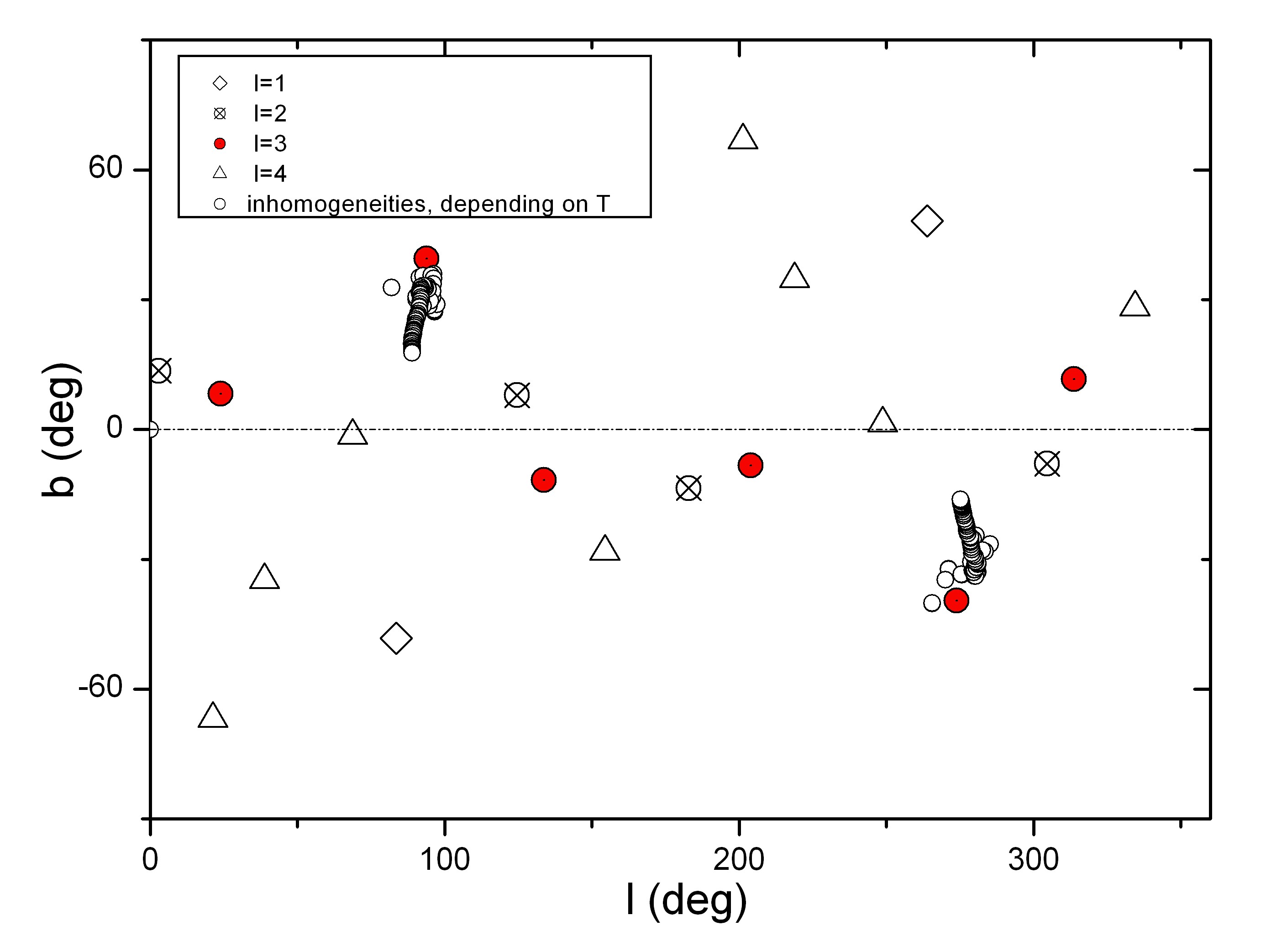
Figure 1: Drift of the centers A and B with the increase of the temperature threshold interval and the multipole vectors $\ell=1-4$.

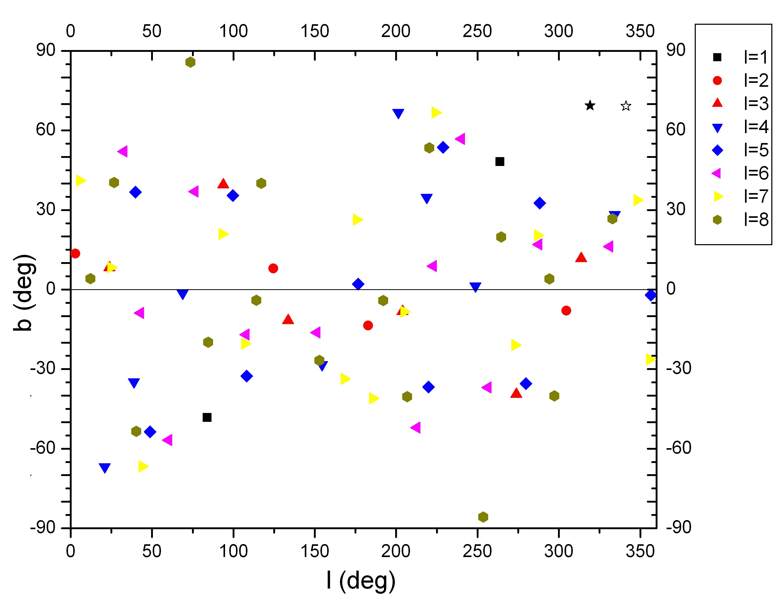
Figure 2: Multipole vectors, $\ell=1-8$, and the sum vectors, $\ell=1-8$ (black star) and $\ell=2-8$ (open star).

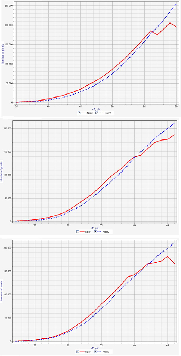
Figure 3: Pixel numbers of the excursion sets vs the radius from A and B (dotted line) at temperature step 1 $\mu K$ (upper plot). The middle and lower plots are with $\ell=2$ and $\ell=2,3$ multipoles removed, respectively.

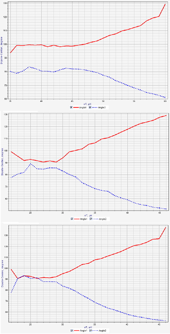
Figure 4: The distance of the dipole apexes from A,B; the rest as is in previous figure. The $\chi^{2}$ for mirroring is 1.50, 1.48, 4.81, respectively.

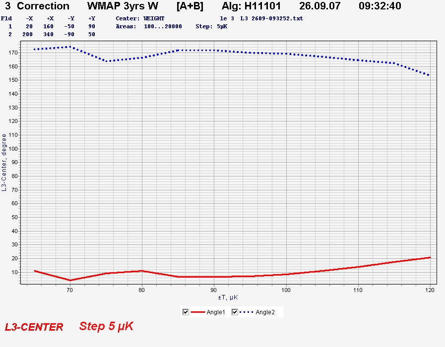
Figure 5: The distance of $\ell=3$ (closest vector) from A,B; mirorring $\chi^{2}=0.74$.

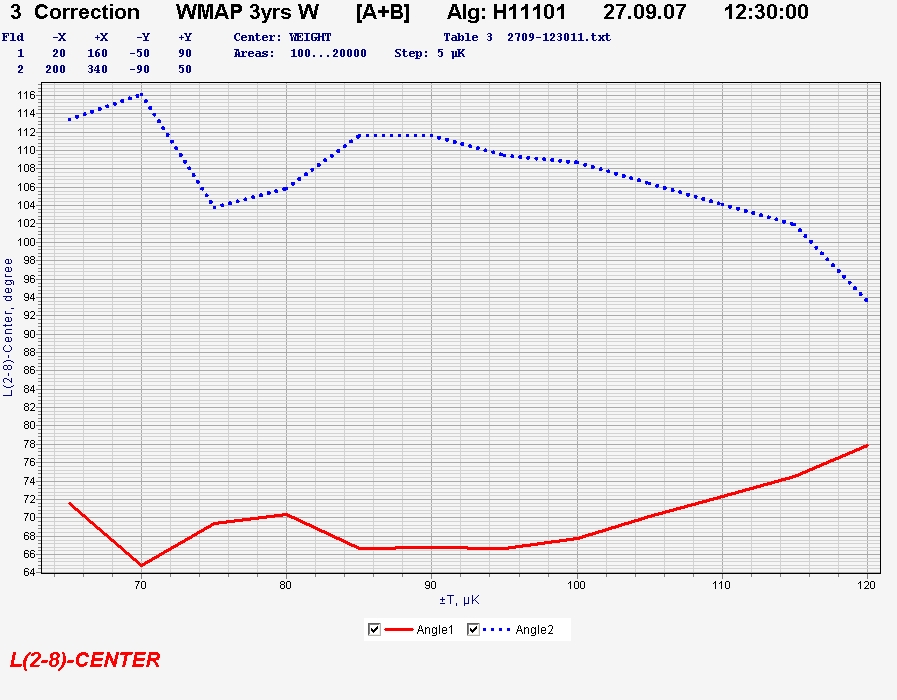
Figure 6: The distance of $\ell=2-8$ sum vector from A,B; mirroring $\chi^{2}=0.78$.

5 Discussion

The centers of excursion sets have nearly antipodal locations. The inhomogeneity centers are close to one of $\ell=3$ multipole vectors, but not close to the sum vector of multipoles up to $\ell=8$. They are close to the ecliptic pole and are nearly orthogonal to the CMB dipole apexes; however, they drift upon the increase of the temperature threshold interval. The effect weakens, but does not disappear completely when the $\ell=2$ or $\ell=2,3$ modes are extracted. There are visible mirroring properties, even if not perfect.

The association to these inhomogeneities with mirroring features either to the ecliptic, or to the dipole or to the l=3 multipole, i.e. to unknown interplay of interplanetary and Galactic foregrounds is certainly a central issue. In that case, however, one is led to reconsider such non-cosmological contributions in the low multipoles. For now, this seems one of the strong alternatives.

What if the described features are nevertheless cosmological? Do there exist fundamental mechanisms producing such an approximate mirror symmetry of CMB temperature fluctuations with respect to some fixed plane, apart from a pure chance? The answer is positive, and the simplest possibility is presented by the non-trivial spatial topology of the Universe of the $T^{1}$ type, i.e. with one of spatial coordinates, say $z$, being identified: $z\equiv z+L$. This topology may be considered as a limiting case of the Universe with compact flat spatial sections having the $T^{3}$ topology if the identification scales $L_{1},L_{2}$ along two other spatial coordinates are much more than $L$ (the slab topology), see [16, 17, 18] for the discussions of quantum creation of the early universe with such topology. Another possibility is to have compact positively curved spatial sections with the radius of curvature much exceeding the present cosmological horizon $R_{hor}$ (so that $\Omega_{tot}-1\ll 1$) and with the topology $S^{3}/Z_{N},~{}N\gg 1$.

As was shown in [19], in the case of the $T^{1}$ spatial topology oriented along the $z$ axis, a large-angle pattern of a CMB temperature anisotropy $\Delta T(\theta,\phi)$ is a sum of two terms. The first of them has the exact plane (mirror) symmetry with respect to the $(x,y)$ plane, namely

$$\Delta T(\theta,\phi)=\Delta T(\pi-\theta,\phi).$$ (6)

It originates from the Sachs-Wolfe effect at the large scattering surface from density perturbations which does not depend on $z$. The second term represents the remaining part of anisotropy and does not have any symmetry at all. However, for $a_{0}L$ of the order of $R_{\rm hor}$ or slightly more, where $a_{0}=a(t_{0})$ is the present scale factor of a Friedmann-Robertson-Walker cosmological model, the latter term should be somehow suppressed since the Sachs-Wolfe contribution to it from the last scattering surface comes from perturbations having wave vectors with $|{\bf k}|\geq 2\pi/L$. That is why we can expect a total large-angle pattern of $\Delta T$ to have an approximate mirror symmetry in this case which should quickly disappear at smaller angles.

The first direct search for such an effect in [20] using the COBE data with a negative result placed a lower bound of the topological scale $a_{0}L>3h^{-1}~{}{\rm Gpc}~{}\approx 0.3R_{\rm hor}$ at the $95\%$ confidence (the value of $R_{\rm hor}$ is given for $\Omega_{m}=0.3,~{}\Omega_{\Lambda}=0.7$). Using the first-year WMAP data and adding a different, ”circles on the sky” method, this upper bound was raised up to $\sim R_{hor}$ [3] and then even up to $\approx 1.8R_{hor}$ [21], see also [22, 23, 24].

However, even $a_{0}L\geq 2R_{hor}$ (when the circles in the sky method does not work at all) does not exclude observability of this effect, if the $z$-independent large-scale part of 3D perturbations has a sufficiently large amplitude. It should be emphasized that there is no definite prediction of a relative amplitude of this ’zero’ mode of perturbations compared to a generic mode with $k_{z}\not=0$ since there is no definite theory of how this topology arises. Moreover, the recent re-analysis of this problem for the cubic $T^{3}$ topology ($L=L_{1}=L_{2}$) (for which there may be no approximate mirror symmetry at all) using the three-year WMAP data [25] suggests that the lower limit in [21] is too optimistic, so even $a_{0}L=1.2R_{\rm hor}$ is not excluded in this case (in agreement with the lower limit obtained earlier in [26]). Clearly, a lower limit on $a_{0}L$ for the $T^{1}$ topology may not be less than that for the more restrictive cubic $T^{3}$ topology, so $a_{0}L\geq 1.2R_{\rm hor}$ seems to be still possible for the former topology, too. Note also that a possible mirror symmetry of the Universe was proposed in [27], however, with suppression of even multipoles (odd point parity).

Thus, even though obtaining of secure constraints either on the torus topology or the compactification scales needs further data and efforts, the large scale non-perfect mirroring in the CMB maps revealed above, if cosmological, would already indicate that the large-scale $z$-independent part of density perturbation inside our cosmological horizon is anomalously large.

We thank Paolo de Bernardis for valuable discussions and help. AAS was partially supported by the Research Program “Astronomy” of the Russian Academy of Sciences. He also thanks Prof. Remo Ruffini and ICRANet, Pescara for hospitality during the final stage of this project.

References

- [1] P. de Bernardis et al., Nature 404 (2000) 955
- [2] D. Spergel et al., Astroph. J. Suppl. 170 (2007) 377
- [3] A. de Oliveira-Costa et al., Phys. Rev. D 69 (2004) 063516
- [4] C.J. Copi, D. Huterer and G.D. Starkman, Phys. Rev. D 70 (2004) 043515
- [5] D.J. Schwarz, D. Huterer, G.D. Starkman and C.J. Copi, Phys. Rev. Lett. 93 (2004) 221301
- [6] H. Eriksen et al. Astroph. J. 612 (2004) 633
- [7] C.J. Copi, D. Huterer, D.J. Schwarz, G.D. Starkman, Mon. Not. Roy. Astron. Soc. 367 (2006) 79
- [8] M.R. Dennis, J. Phys. A 38 (2005) 1653
- [9] R.C. Helling, P. Schupp and T.Tesileanu, Phys.Rev. D74 (2006) 063004
-
[10]
V.G. Gurzadyan, P.A.P. Ade, P. de Bernardis et al.,
Int.J.Mod.Phys. D12 (2003) 1859;
V.G. Gurzadyan, P. de Bernardis et al., Mod.Phys.Lett. A20 (2005) 893 - [11] V.G. Gurzadyan, C.L. Bianco et al., Phys.Lett. A 363 (2007) 121
- [12] V.G. Gurzadyan and S. Torres, A & A 321 (1997) 19
- [13] K. Karcher, in: Chern, Global Differential Geometry, p.170, 1989; M. Berger, A Panoramic View of Riemannian Geometry, Springer (2003).
- [14] Gorski, K.M., Hivon, E. and Wandelt, B.D., 1998, astro-ph/9812350; http://www.eso.org/kgorski/healpix/
- [15] P. Vielva et al., Astroph. J. 609 (2004) 22
- [16] Ya.B. Zeldovich and A.A. Starobinsky, Sov. Astron. Lett. 10 (1984) 135
- [17] V.G. Gurzadyan and A.A. Kocharyan, Sov. Phys. - JETP 68 (1989) 1.
- [18] A.D. Linde, JCAP 0410 (2004) 004 (arXiv:hep-th/0408164)
- [19] A.A. Starobinsky, JETP Lett. 57 (1993) 622 (arXiv:gr-qc/9305019)
- [20] A. de Oliveira-Costa, G.F. Smoot and A.A. Starobinsky, Astroph. J. 468 (1996) 457 (arXiv:astro-ph/9510109)
- [21] N.J. Cornish, D.N. Spergel, G.D. Starkman and E. Komatsu, Phys. Rev. Lett. 92 (2004) 201302 (arXiv:astro-ph/0310233)
- [22] M. Kunz, N. Aghanim, L. Cayon et al., Phys. Rev. D 73 (2006) 023511 (arXiv: astro-ph/0510164)
- [23] J.G. Cresswell, A.R. Liddle, P. Mukherjee and A. Riazuelo, Phys. Rev. D 73 (2006) 041302 (arXiv:astro-ph/0512017)
- [24] R. Aurich, S. Lustig, F. Steiner and H. Then, Class. Quant. Grav. 24 (2007) 1879 (astro-ph/0612308)
- [25] R. Aurich, H.S. Janzer, S. Lustig and F. Steiner, 2007, arXiv:0708.1420 [astro-ph]
- [26] N.G. Philips and A. Kogut, Astroph. J. 645 (2006) 820 (arXiv:astro-ph/0404400)
- [27] K. Land and J. Magueijo, Phys. Rev. D 72 (2005) 101302 (arXiv:astro-ph/0507289)