A polydisperse lattice-gas model

Abstract

We describe a lattice-gas model suitable for studying the generic effects of polydispersity on liquid-vapor phase equilibria. Using Monte Carlo simulation methods tailored for the accurate determination of phase behaviour under conditions of fixed polydispersity, we trace the cloud and shadow curves for a particular Schulz distribution of the polydisperse attribute. Although polydispersity enters the model solely in terms of the strengths of the interparticle interactions, this is sufficient to induce the broad separation of cloud and shadow curves seen both in more realistic models and experiments.

I Introduction

Lattice-based models of many-body systems have been in the vanguard of the drive for an improved understanding of equilibrium phase behaviour, almost since the inception of the field CL . The utility of such models derives both from the simplifications to approximate analytical treatments that result from the spatial discretisation, and from their amenability to efficient numerical simulation. Indeed, even in the current era of teraflop computers, simulations of lattice models are still deployed routinely in fields as diverse as polymer physics and quantum chromodynamics.

The purpose of this paper is to introduce a new lattice-gas model suitable for simulation investigations of the phase behaviour of polydisperse fluids. These are complex fluids whose constituent particles exhibit continuous variation in terms of some physical attribute such as their size, shape or charge. Polydispersity is inherent to a host of natural and synthetic soft matter fluids including (inter alia) colloidal dispersions, polymer solutions, liquid crystals, as well as some biological fluids such as blood larson1999 . Understanding its generic effects on the phase behaviour of model systems is, therefore, not only a matter of fundamental interest, but also one of considerable practical and commercial importance.

The complexity bestowed on a fluid system by polydispersity complicates simulation studies of phase behaviour. Although newly-developed methodologies wilding2002d ; wilding2003a ; buzzacchi2006 ; Wilding2006 allow the accurate study of phase coexistence in off-lattice models of polydisperse fluids, progress has nevertheless been hindered (compared to studies of monodisperse systems) by the fact that coexistence occurs over a region of the pressure-temperature phase diagram, rather than merely along a line Bellier-castella2002 ; Rascon2003 . The necessity of exploring a higher dimensional space of model parameters in order to fully characterize a given phase transition renders such investigations laborious. Hence progress in elucidating the generic effects of polydispersity on phase behaviour has been slower than be might be desired.

Accordingly, there is a pressing need for a computationally tractable model system, which, whilst not necessarily portraying realistically the microscopic features of any particular polydisperse fluid, does nevertheless capture principal features of the macroscopic phase behaviour. The lattice-gas model presented below should go some way to meeting this need. Specifically, it should help answer unsolved questions such as how the coexistence and critical point properties depend on the nature of the particle interactions and the form and degree of the polydispersity. Additionally it should provide an efficient test bed for the development of fresh computational and analytical methodologies for studying polydisperse phase behaviour.

The structure of our paper is as follows. In Sec. II we outline salient features of the phase behaviour of polydisperse systems, before moving on to describe the polydisperse lattice-gas (PLG) model in Sec. III. We then report, in Sec. IV, a simulation study of key features of the liquid-vapor phase behaviour for one particular choice of the form of the polydispersity. Finally, Sec. V summarizes our findings and conclusions.

II Background: polydisperse phase equilibria

In this section we present a brief overview of the principal differences between phase coexistence in polydisperse and monodisperse systems, For a more detailed discussion, the interested reader is referred to a recent review sollich2002 .

The state of a polydisperse system (or any of its phases) is described by a density distribution $\rho(\sigma)$, with $\rho(\sigma)d\sigma$ the number density of particles whose polydisperse attribute $\sigma$ lies in the range $\sigma\ldots\sigma+d\sigma$. In the most commonly encountered experimental situation, the form of the overall or “parent” distribution, $\rho^{(0)}(\sigma)$, is fixed by the synthesis of the fluid, and only its scale can vary depending on the proportion of the sample volume occupied by solvent. One can then write $\rho^{(0)}(\sigma)=n^{(0)}f^{(0)}(\sigma)$ where $f^{(0)}(\sigma)$ is the normalized parent shape function and $n^{(0)}=N/V$ the overall particle number density; as the latter is varied, $\rho^{(0)}(\sigma)$ traces out a “dilution line” in density distribution space. The phase diagram is then spanned by $n^{(0)}$ and the temperature $T$.

The richness of the phase behaviour of polydisperse fluids stems from the occurrence of fractionation evans2001 ; fairhurst2004 ; erne2005 : at coexistence, particles of each $\sigma$ may partition themselves unevenly between two or more “daughter” phases as long as–due to particle conservation–the overall density distribution $\rho^{(0)}(\sigma)$ of the parent phase is maintained. As a consequence, the conventional vapor-liquid binodal of a monodisperse system splits into a cloud curve marking the onset of coexistence, and a shadow curve giving the density of the incipient phase; the critical point appears at the intersection of these curves rather than at the maximum of either sollich2002 . This splitting is seen in experiments on polydisperse fluids (see e.g. ref. Borchard1994 ).

The daughter distributions are related to the parent via a simple volumetric average: $(1-\xi)\rho^{(1)}(\sigma)+\xi\rho^{(2)}(\sigma)=\rho^{(0)}(\sigma)\>,$ where $1-\xi$ and $\xi$ are the fractional volumes of the two phases. In contrast to a monodisperse system where the densities of the coexisting phases are specified by the binodal and depend solely on temperature, full specification of the coexistence properties of a polydisperse system requires not only knowledge of the cloud curve, but also the dependence of $\xi$, $\rho^{(1)}(\sigma)$ and $\rho^{(2)}(\sigma)$ on $n^{(0)}$ and $T$ buzzacchi2006 .

III Polydisperse lattice-gas model

Our polydisperse lattice-gas (PLG) model is defined within the grand canonical ensemble by the hamiltonian:

$$H=-\sum_{(ij),\sigma,\sigma^{\prime}}(\sigma\sigma^{\prime})^{\alpha}c_{i}(\sigma)c_{j}(\sigma^{\prime})-\sum_{i,\sigma}\mu(\sigma)c_{i}(\sigma).$$ (1)

Here $\sigma$ is the value (assumed scalar) of the polydisperse attribute, which controls the strength of interparticle interactions. We shall regard $\sigma$ as the label for a notional particle “species”, whose corresponding chemical potential is $\mu(\sigma)$. The exponent $\alpha$ can, in principle, take an arbitrary value but we shall restrict ourselves to the case $\alpha=1$ in the present study. $c_{i}(\sigma)$ simply counts the number of particles of species $\sigma$ at site $i$, for which we impose a hard-core constraint such that $\sum_{\sigma}c_{i}(\sigma)=0$ or $1$. The instantaneous density distribution follows as $\rho(\sigma)=L^{-d}\sum_{i}c_{i}(\sigma)$, with $d=3$ in the simulations reported below; $i$ runs over the sites of a periodic lattice $i=1,...,L^{d}$, assumed simple cubic in this work. The sum in the first term on the right hand side of (1) similarly runs over all pairs $i$,$j$ of nearest neighbor sites, as well as over all combinations of $\sigma$ and $\sigma^{\prime}$.

Put simply, each lattice site may be either vacant, or occupied by a single particle which carries a continuous species label $\sigma$. Particles on nearest neighbor sites interact with a potential energy which is the negative of the product of their species labels. Thus the role of polydispersity in this model is to engender a spread of possible interaction strengths between particles –a situation which contrasts with the single interaction strength characterizing the simple Ising lattice-gas model BINNEY .

The model of Eq. 1 (which we have also briefly described in a different context elsewhere buzzacchi2006 ) has, to our knowledge, not been considered previously by other authors. We note that it is distinct from well-known lattice spin models such as the $q$-state Potts model in the limit of large $q$, and the $XY$ model. The distinction arises both in terms of the form of the interactions, and the absence of an isomorphic magnetic description, in contrast to the case of the simple (monodisperse) lattice-gas BINNEY .

IV Simulation studies

IV.1 Parent distribution

In this work we consider the case in which the species labels $\sigma$ are drawn stochastically from a (parental) distribution of the Schulz form Schulz1939 :

$$f^{(0)}(\sigma)=\frac{1}{z!}\left(\frac{z+1}{\bar{\sigma}}\right)^{z+1}\sigma^{z}\exp\left[-\left(\frac{z+1}{\bar{\sigma}}\right)\sigma\right]\>,$$ (2)

with a mean species label $\bar{\sigma}\equiv 1$. We have elected to study the case $z=50$, corresponding to a moderate degree of polydispersity: the standard deviation of the species label is $\delta\equiv 1/\sqrt{z+1}\approx 14\%$ of the mean. The form of the distribution is shown in Fig. 1. Although our motivation for employing the Schulz distribution is primarily ad-hoc, we note that it has been found to fairly accurately describe the polydispersity of some polymeric systems McDonnell2003 .

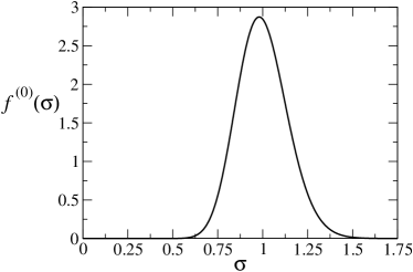
Figure 1: The Schulz parent distribution for the case $z=50$ (cf. Eq. (2)).

In the simulations reported below, the distribution $f^{(0)}(\sigma)$ was limited for computational convenience to the range $0.5<\sigma<1.4$, and renormalized appropriately. Imposition of lower and upper cutoffs, in the tails of the parent distribution, obviates the need to determine the associated portions of the chemical potential distribution $\mu(\sigma)$ conjugate to $\rho^{(0)}(\sigma)$ – a task that can be numerically fraught when the parent density is very small. It should be noted, however, that depending on the form of the parent, the upper cutoff can have drastic effects on the phase behaviour, even when it is located far into the tail of the distribution wilding2005b .

IV.2 Methodology

We have studied the phase behaviour of the PLG model, Eq. 1, under conditions of fixed polydispersity via Monte Carlo simulations within the grand canonical ensemble (GCE). Our Metropolis algorithm invokes three types of lattice operations: particle deletions, particle insertions, and variation of a particle’s species label $\sigma$. The latter quantity is treated as a continuous variable in the permitted range $0.5<\sigma<1.4$; however, distributions defined on $\sigma$, such as the instantaneous density $\rho(\sigma)$, and the chemical potential $\mu(\sigma)$, are represented as histograms formed by discretising this range into $100$ bins. The simulation results presented below pertain to periodic cubic systems of linear dimension $L=10,20,30,40$ lattice units. Further details concerning general aspects of the simulation of polydisperse fluids within the GCE, as well as the structure, storage and acquisition of data, have been presented elsewhere wilding2002d .

The principal observable of interest is the fluctuating form of the instantaneous density distribution $\rho(\sigma)$. From this we derive the distribution $p(n)$ of the overall number density $n=\int d\sigma\rho(\sigma)$. If one further identifies $\sigma$ with particle diameter – subject to the proviso that our model does not account for any diameter dependence of the hard core repulsion – we can consider, as an alternative to the density $n$, a notional “volume fraction” $\eta=(\pi/6)\int d\sigma\sigma^{3}\rho(\sigma)$.

The existence of phase coexistence at given chemical potentials is signalled by the presence of two distinct peaks in the probability distribution $p(n)$. In order to obtain estimates of dilution line coexistence properties at some prescribed temperature, we employ an accurate approach recently proposed by ourselves buzzacchi2006 . For a given choice of $n^{(0)}$, the method entails tuning the chemical potential distribution $\mu(\sigma)$ together with a parameter $\xi$, such as to simultaneously satisfy both a generalized lever rule and an equal peak weight criterion borgs1992 for $p(n)$:

$$n^{(0)}f^{(0)}(\sigma) = (1-\xi)\rho^{(1)}(\sigma)+\xi\rho^{(2)}(\sigma)$$ (3a)

$$r = 1$$ (3b)

Here the daughter density distributions $\rho^{(1)}(\sigma)$ and $\rho^{(2)}(\sigma)$ are assigned by averaging only over configurations belonging to either peak of $p(n)$. The quantity $r$ is the peak weight ratio:

$$r=\frac{\int_{n>n^{*}}p(n)dn}{\int_{n<n^{*}}p(n)dn}\>,$$ (4)

with $n^{*}$ a convenient threshold density intermediate between vapor and liquid densities, which we take to be the location of the minimum in $p(n)$. The tuning of $\mu(\sigma)$ and $\xi$ necessary to simultaneously satisfy Eqs. (3a) and (3b) can be efficiently achieved by histogram extrapolation techniques Ferrenberg1989 , given an initial estimate for $\mu(\sigma)$ which is provided by an iterative refinement technique, as described elsewhere wilding2003a .

The value of $\xi$ resulting from the application of the above procedure is the desired fractional volume of the liquid phase at the nominated value of $n^{(0)}$. Cloud points are determined as the value of $n^{(0)}$ at which $\xi$ first reaches zero (vapor branch) or unity (liquid branch), while shadow points are given by the density of the coexisting incipient daughter phase, which may be simply read off from the appropriate peak position in the cloud point form of $p(n)$ and $p(\eta)$. It should be pointed out that the finite-size corrections to estimates of coexistence properties obtained using the equal peak weight criterion for $p(n)$ are exponentially small in the system size buzzacchi2006 .

In order to obtain the phase behaviour of our model system, we scanned the dilution line for a selection of fixed temperatures. We started by setting $T=T_{c}$, the critical temperature (known from a brief preliminary study buzzacchi2006 ), and tracked the locus of the dilution line in a stepwise fashion. This tracking procedure must be bootstrapped with knowledge of the form of $\mu(\sigma)$ at some initial point on the dilution line. A suitable estimate was obtained, for a point near the critical density, by means of the iterative refinement procedure wilding2003a , in conjunction with the equal peak weight criterion for $p(n)$ discussed above. Simulation data accumulated at this near-critical state point was then extrapolated to a lower, but nearby density $n^{(0)}$ by means of histogram reweighting, thus providing an estimate of the corresponding form of $\mu(\sigma)$. The latter was employed in a new simulation, the results of which were similarly extrapolated to a still lower value of $n^{(0)}$. Iterating this procedure thus enabled the systematic tracing of the whole dilution line and the identification of cloud points. Histogram extrapolation further permitted a determination of dilution line properties at adjacent temperatures, thereby facilitating a systematic determination of the phase behaviour in the $n^{(0)}-T$ plane, including special loci such as the cloud curve and the critical isochore ($n^{(0)}=n^{(0)}_{c}$). Implementation of multicanonical preweighting techniques berg1992 at each coexistence state point ensured adequate sampling of the coexisting phases in cases where they are separated by a large interfacial free energy barrier. A fuller account of this latter procedure has been presented previously wilding2001 .

IV.3 Results

The techniques outlined above were used to obtain accurate estimates of key features of the phase diagram of the PLG, namely the cloud and shadow curves, and the coexistence properties on the critical isochore.

The liquid-vapor critical point has been located approximately in a previous brief study of the PLG buzzacchi2006 , which found $(n^{(0)}_{c},T_{c})=(0.521,1.171)$ in reduced units. This is to be compared with the critical parameters of the monodisperse (Ising) lattice-gas $(0.5,1.127955)$ Luijten1995 . Thus the inclusion of polydispersity of the form (1) is seen to raise both the critical temperature and the critical density. Moreover we find that it splits the liquid-vapor binodal into well-separated cloud and shadow curves (cf. Fig. 2) in a manner similar to that occurring in continuum fluid models for which polydispersity affects the interparticle interaction strength as well as its range wilding2005b ; Wilding2006 . (When only the range is polydisperse, a scale symmetry forces the critical point to be near the top of cloud and shadow sollich07 ; bellier-Castella2000 ; wilding2004a ; wilding2004b .) As a consequence, the critical point lies below the maximum of the cloud curve and phase coexistence can be observed even at $T=T_{c}$, provided that $n^{(0)}<n^{(0)}_{c}$. Note that our procedure for cloud/shadow curve determination breaks down in the vicinity of the critical point, because the two peaks in $p(n)$ overlap in a finite-sized system. This is the reason for absence of data near criticality in Fig. 2.

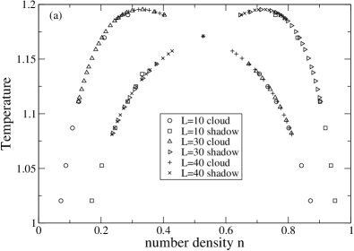
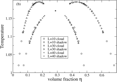
Figure 2: Estimates of the cloud and shadow curves of the PLG model for the Schulz parent distribution of Eq. 2, obtained as described in the text. Data are shown for three system sizes. (a) Density-temperature plane. (b) Volume fraction-temperature plane. In each case the estimated critical point is marked by a star ($\star$).

Fig. 3 shows the normalized forms of the vapor and liquid daughter phase distributions for a point on the cloud curve well away from criticality. One sees that in keeping with previous findings for off-lattice models wilding2005b ; Wilding2006 , there is considerable fractionation. Specifically, the number of particles in the liquid phase having a large value of $\sigma$ is strongly enhanced relative to the vapor phase. This enhancement arises because particles having larger $\sigma$ interact more strongly than those of small $\sigma$, thereby yielding a substantial free energy gain of the liquid (with its larger number of nearest neighbor particle contacts) over the vapor. One further sees that as a result of this enhancement, the form of the liquid daughter phase distribution is strongly affected by the presence of the cutoff. The issues surrounding such “cutoff effects” and their implications for phase behaviour have recently been examined in detail in refs. wilding2005b ; Wilding2006 .

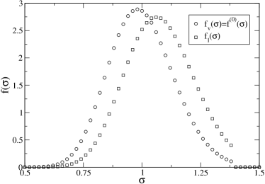
Figure 3: Normalized daughter distributions $f_{v}(\sigma)$ and $f_{l}(\sigma)$ for the vapor ($v$) and liquid ($l$) phases as obtained for the $L=30$ system on the cloud curve at $n^{(0)}=0.1275,T=1.111$, as described in the text.

Finally, in this section, we have determined the coexistence curve corresponding to a parent density which is fixed at its critical value $n^{(0)}_{c}=0.521$. This curve is presented in Fig. 4. One notes that its general shape is similar to the standard binodal that one finds in a monodisperse fluid. This is because the fractional volumes of the two phases are approximately (though not strictly) equal on this coexistence curve. By contrast, on the cloud curve the fractional volume of one phase is infinitesimal, leading to much stronger fractionation effects.

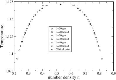
Figure 4: Estimates of the coexistence curve for which the parent density $n^{(0)}$ is fixed to its critical point value ie. $n^{(0)}=n^{(0)}_{c}$. Data is shown for three system sizes. The marked densities at each temperature derive from the peak positions in the corresponding form of $p(n)$. Clear finite-size effects are visible in the vicinity of the critical point.

V Conclusions

In this paper, we have introduced a lattice-gas model for a polydisperse fluid and shown that it exhibits qualitatively similar liquid-vapor phase behaviour to realistic continuum fluid models in which polydispersity affects both the size and the strength of the particle interactions wilding2005b ; Wilding2006 . In tests we find that the coexistence properties of the PLG can be determined with a computational effort that is smaller by a factor of $1-2$ orders of magnitude compared to that for an off-lattice system having a similar number of particles at equivalent state points such as criticality. This bodes well for the prospects of harnessing the PLG model to elucidate how coexistence properties are affected by factors such as the form of the parent distribution, the choice of the large-$\sigma$ cutoff to the parent distribution, and the $\sigma$-dependence of the interaction strength (which is controlled in the PLG by the exponent $\alpha$ in Eq. 1). Additionally the model, and the results we have provided, may prove useful as a computationally efficient test bed for anyone wishing to “tool-up” for simulation studies of polydispersity on other systems.

Finally we note that experiments have been performed on polydisperse polymers which report that the critical exponents for the critical coexistence curve are Fisher-renormalized with respect to the standard Ising values kita1997a . The present model may provide a useful platform for elucidating these intriguing findings; this is something which we hope to do in future work.

References

- (1) P.M. Chaikin and T.C. Lubensky, Principles of Condensed Matter Physics (Cambridge U.P, Cambridge, Cambridge, 1995).
- (2) R.G. Larson, The structure and rheology of complex fluids (Oxford University Press, New York, 1999).
- (3) N.B. Wilding and P Sollich, J. Chem. Phys. 116, 7116 (2002).
- (4) N.B. Wilding, J. Chem. Phys. 119, 12163 (2003).
- (5) M. Buzzacchi, P. Sollich, N.B. Wilding, and M. Müller, Phys. Rev. E. 73, 046110 (2006).
- (6) M. Fasolo N.B. Wilding, P. Sollich and M. Buzzacchi, J. Chem. Phys. 125, 014908 (2006).
- (7) L Bellier-Castella, H Xu, and M Baus, Phys. Rev. E. 65, 021503 (2002).
- (8) C. Rascon and M.E. Cates, J. Chem. Phys. 118, 4312 (2003).
- (9) P. Sollich, J. Phys.: Condens. Matter 14, R79 (2002).
- (10) R.M.L. Evans, J. Chem. Phys. 114, 1915 (2001).
- (11) D.J. Fairhurst and R.M.L. Evans, Colloid And Polymer Science 282, 766 (2004).
- (12) B.H. Erne et al., Langmuir 21, 1802 (2005).
- (13) W. Borchard, S. Frahn, and V. Fischer, Macromolecul. Chem. Phys. 195, 3311 (1994).
- (14) J.J. Binney, N.J. Dowrick, A.J. Fisher, and M.E.J Newman, The Theory of Critical Phenomena (Oxford U.P., Oxford, 1992).
- (15) G.V. Schulz, Z. Phys. Chem. Abt. B 43, 25 (1939).
- (16) M. E. McDonnell and A. M. Jamieson, J. Appl. Polym. Sci. 21, 3261 (2003).
- (17) N.B. Wilding, P Sollich, and M Fasolo, Phys. Rev. Lett. 95, 155701 (2005).
- (18) C. Borgs and R. Kotecky, Phys. Rev. Lett. 68, 1734 (1992).
- (19) A.M. Ferrenberg and R.H. Swendsen, Phys. Rev. Lett. 63, 1195 (1989).
- (20) B.A. Berg and T. Neuhaus, Phys. Rev. Lett. 68, 9 (1992).
- (21) N.B. Wilding, Am. J. Phys. 69, 1147 (2001).
- (22) H.W.J. Blöte, E. Luijten, and J.R. Heringa, J. Phys. A 28, 6289 (1995).
- (23) P. Sollich, preprint (2007).
- (24) L Bellier-Castella, H Xu, and M Baus, J. Chem. Phys. 113, 8337 (2000).
- (25) N.B. Wilding, M Fasolo, and P Sollich, J. Chem. Phys. 121, 6887 (2004).
- (26) N.B. Wilding and P Sollich, Europhysics Letters 67, 219 (2004).
- (27) R. Kita, T. Dobashi, T. Yamamoto, M. Nakata and K. Kamide, Phys. Rev. E. 55, 3159 (1997).